Volume 3, Issue 6 e1163

SPECIAL ISSUE PAPER

Full Access

Solving fully randomized higher-order linear control differential equations: Application to study the dynamics of an oscillator

Juan-Carlos Cortés,

Juan-Carlos Cortés

orcid.org/0000-0002-6528-2155

Instituto Universitario de Matemática Multidisciplinar, Universitat Politècnica de València, Valencia, Spain

Search for more papers by this author

Ana Navarro-Quiles,

Ana Navarro-Quiles

orcid.org/0000-0003-3800-072X

Department of Statistics and Operational Research, Universitat de València, Burjassot, Spain

Search for more papers by this author

José-Vicente Romero,

José-Vicente Romero

orcid.org/0000-0003-3366-6557

Instituto Universitario de Matemática Multidisciplinar, Universitat Politècnica de València, Valencia, Spain

Search for more papers by this author

María-Dolores Roselló,

Corresponding Author

María-Dolores Roselló

[email protected]

orcid.org/0000-0002-5724-7683

Instituto Universitario de Matemática Multidisciplinar, Universitat Politècnica de València, Valencia, Spain

Correspondence María-Dolores Roselló, Instituto Universitario de Matemática Multidisciplinar, Universitat Politècnica de València, Camino de Vera s/n, 46022 Valencia, Spain.

Email: [email protected]

Search for more papers by this author

Juan-Carlos Cortés,

Juan-Carlos Cortés

orcid.org/0000-0002-6528-2155

Instituto Universitario de Matemática Multidisciplinar, Universitat Politècnica de València, Valencia, Spain

Search for more papers by this author

Ana Navarro-Quiles,

Ana Navarro-Quiles

orcid.org/0000-0003-3800-072X

Department of Statistics and Operational Research, Universitat de València, Burjassot, Spain

Search for more papers by this author

José-Vicente Romero,

José-Vicente Romero

orcid.org/0000-0003-3366-6557

Instituto Universitario de Matemática Multidisciplinar, Universitat Politècnica de València, Valencia, Spain

Search for more papers by this author

María-Dolores Roselló,

Corresponding Author

María-Dolores Roselló

[email protected]

orcid.org/0000-0002-5724-7683

Instituto Universitario de Matemática Multidisciplinar, Universitat Politècnica de València, Valencia, Spain

Correspondence María-Dolores Roselló, Instituto Universitario de Matemática Multidisciplinar, Universitat Politècnica de València, Camino de Vera s/n, 46022 Valencia, Spain.

Email: [email protected]

Search for more papers by this author

First published: 06 April 2021

https://doi.org/10.1002/cmm4.1163

Citations: 1

Funding information: European Social Fund, GJIDI/2018/A/009; GJIDI/2018/A/010; Spanish Ministerio de Economía, Industria y Competitividad (MINECO), the Agencia Estatal de Investigación (AEI) and Fondo Europeo de Desarrollo Regional (FEDER UE), MTM2017-89664-P

Share a link

Email
Wechat
Bluesky

Abstract

In this work, we consider control problems represented by a linear differential equation assuming that all the coefficients are random variables and with an additive control that is a stochastic process. Specifically, we will work with controllable problems in which the initial condition and the final target are random variables. The probability density function of the solution and the control has been calculated. The theoretical results have been applied to study, from a probabilistic standpoint, a damped oscillator.

1 INTRODUCTION

The aim of control theory is to ensure that a system subject to perturbations can remain under a specific trajectory. This interdisciplinary branch of engineering and mathematics has many applications in both areas.^1-3 An important part of control theory is devoted to study systems that obey the so-called superposition principle, that is, linear systems.⁴ A linear differential equation with additive control can be written in the form

x^{(n)} (t) + a_{n - 1} x^{(n - 1)} (t) + \dots + a_{0} x (t) = u (t),

()

where x(t) denotes the state variable at the time instant t and u(t) is the control. In this context, it is important to note that a system is said to be controllable if any final state can be reached from any initial state in a control time T > 0. The values of coefficients (also called model parameters), a_i, 0 ≤ i ≤ n − 1, that appear in the formulation are usually set experimentally. As a consequence, these values may contain an intrinsic uncertainty. So it is more convenient to treat model parameters as random variables (RVs) or stochastic processes (SPs) in dealing with control problems.^5-8 In this setting, the solution x = x(t) and the control u = u(t) are SPs defined on a common complete probability space

(Ω, ℱ, ℙ)

. Thus, they are denoted by

x (t, ω)

and

u (t, ω)

, respectively, being

(t, ω) \in (0, T] \times Ω

. Unlike the deterministic theory, in the setting of random control theory, besides computing

x (t, ω)

and

u (t, ω)

, it is important to determine their main statistical properties, in particular the mean,

μ_{x} (t)

, and the variance,

σ_{x}^{2} (t)

. A more desirable objective is to obtain the so-called first probability density functions (1-PDFs), f₁(x, t) and f₁(u, t), of the solution SP,

x (t, ω)

, and of the control SP,

u (t, ω)

, respectively. From the 1-PDF, the mean, the variance, and other statistics can be calculated by integration. For example, in the case of the solution SP,

μ_{x} (t) = 𝔼 [x (t, ω)] = \int_{ℝ} x f_{1} (x, t) d x, σ_{x}^{2} (t) = 𝔼 [{(x (t, ω))}^{2}] - {(𝔼 [x (t, ω)])}^{2} = \int_{ℝ} x^{2} f_{1} (x, t) d x - {(μ_{x} (t))}^{2},

()

here

𝔼 [\cdot]

stands for the expectation operator. Also, from the 1-PDF one can calculate the probability that the solution SP lies on a particular set of interest

ℙ [a \leq x (t, ω) \leq b] = \int_{a}^{b} f_{1} (x, t) d x .

The main objective of this contribution is to compute the 1-PDF of linear control problems of the form (1) where all the coefficients are RVs and the control is a SP. To do this, the random variable transformation (RVT) method will be applied. RVT is an useful technique to determine the PDF of a RV which comes from mapping another RV whose PDF is given. The multidimensional version of the RVT method is stated in Theorem 1.

Theorem 1. (RVT technique [[9], pp 24–25])Let $X (ω) = {(X_{1} (ω), \dots, X_{m} (ω))}^{⊤}$ and $Z (ω) = {(Z_{1} (ω), \dots, Z_{m} (ω))}^{⊤}$ be two m-dimensional absolutely continuous random vectors defined on a complete probability space $(Ω, ℱ, ℙ)$ . Let $s : ℝ^{m} \to ℝ^{m}$ be a one-to-one deterministic transformation of $X (ω)$ into $Z (ω)$ , that is, $Z (ω) = s (X (ω))$ , $ω \in Ω$ . Assume that s is a continuous mapping and has continuous partial derivatives with respect to each component x_i, 1 ≤ i ≤ m. Then, if f_x(x₁, … , x_m) denotes the joint PDF of the vector $X (ω)$ , and p = s⁻¹ = (p₁(z₁, … , z_m), … , p_m(z₁, … , z_m)) represents the inverse mapping of s = (s₁(x₁, … , x_m), … , s_m(x₁, … , x_m)), the joint PDF of the random vector $Z (ω)$ is given by

f_{Z} (z_{1}, \dots, z_{m}) = f_{X} (p_{1} (z_{1}, \dots, z_{m}), \dots, p_{m} (z_{1}, \dots, z_{m})) |𝒥_{m}|,

where

|𝒥_{m}|

, which is assumed to be different from zero, denotes the absolute value of the Jacobian defined by the following determinant

𝒥_{m} = \det [\begin{array}{ccc} \frac{\partial p_{1} (z_{1}, \dots, z_{m})}{\partial z_{1}} & \dots & \frac{\partial p_{m} (z_{1}, \dots, z_{m})}{\partial z_{1}} \\ ⋮ & ⋱ & ⋮ \\ \frac{\partial p_{1} (z_{1}, \dots, z_{m})}{\partial z_{m}} & \dots & \frac{\partial p_{m} (z_{1}, \dots, z_{m})}{\partial z_{m}} \end{array}] .

In our previous contribution,¹⁰ the random linear control problem

\begin{align} x^{'} (t, ω) & = A (ω) x (t, ω) + B (ω) u (t, ω), 0 < t \leq T, \\ x (0, ω) & = x^{0} (ω), \end{align}

()

has been studied assuming that only the initial condition and the final target are RVs and the control is a SP, since in this case one can take into account the well-known Kalman's controllability condition:

if A and B are matrices of dimensions n × n and n × m, respectively, where m ≤ n, whose elements are deterministic, a necessary and sufficient condition for (A, B) to be controllable is^10-12

rank (C) = rank (B, A B, \dots, A^{n - 1} B) = n,

where C has dimension n × nm and it is referred to as the Kalman's controllability matrix.

We finish this section pointing out that throughout this article the exponential function will be denoted by e or $\exp$ , interchangeably.

2 CONTROLLABLE RANDOMIZED EQUATION

As a natural extension of its deterministic counterpart (1), a linear differential equation whose coefficients are RVs and having an additive stochastic control is given by

x^{(n)} (t, ω) + a_{n - 1} (ω) x^{(n - 1)} (t, ω) + \dots + a_{0} (ω) x (t, ω) = u (t, ω),

()

where

x (t, ω)

is a SP that describes the evolution of the system,

a_{i} (ω)

, i = 0, 1, … , n − 1 are n independent RVs, and

u (t, ω)

is the control term that is assumed to be a SP. All these quantities are defined in a common complete probability space

(Ω, ℱ, ℙ)

In this contribution, we are interested in random controllable problems, this is, given a random initial condition

{x (0, ω) = x_{1}^{0} (ω), x^{'} (0, ω) = x_{2}^{0} (ω), \dots, x^{(n - 1)} (0, ω) = x_{n}^{0} (ω)},

()

we are interested in reaching a random final target

{x (T, ω) = x_{1}^{1} (ω), x^{'} (T, ω) = x_{2}^{1} (ω), \dots, x^{(n - 1)} (T, ω) = x_{n}^{1} (ω)},

()

at a fixed time T > 0. Therefore, we will assume that

x_{i}^{0} (ω), x_{i}^{1} (ω)

, i = 1, … , n, are RVs.

Now, we will establish specific conditions under which the problem (4)–(6) is controllable. For this goal, we will take advantage of Kalman's controllability condition introduced in Section 1. The first step is to recast the random nth-order linear control differential equation (4) as a random first-order linear control system. To this end, we perform the classical change of variables

\begin{align} y_{1} (t, ω) & = x (t, ω), \\ y_{2} (t, ω) & = x^{'} (t, ω), \\ y_{3} (t, ω) & = x^{''} (t, ω), \\ ⋮ \\ y_{n} (t, ω) & = x^{(n - 1)} (t, ω), \end{align}

then, Equation (4) can be rewritten as

y^{'} (t, ω) = A (ω) y (t, ω) + b u (t, ω),

()

where

y (t, ω) = (\begin{array}{c} y_{1} (t, ω) \\ y_{2} (t, ω) \\ ⋮ \\ y_{n - 1} (t, ω) \\ y_{n} (t, ω) \end{array}), b = (\begin{array}{c} 0 \\ 0 \\ ⋮ \\ 0 \\ 1 \end{array}),

()

are n-dimensional vectors and

A (ω) = (\begin{array}{cccccc} 0 & 1 & 0 & \dots & 0 & 0 \\ 0 & 0 & 1 & \dots & 0 & 0 \\ ⋮ & ⋱ & ⋮ \\ 0 & 0 & 0 & \dots & 1 & 0 \\ 0 & 0 & 0 & \dots & 0 & 1 \\ - a_{0} (ω) & - a_{1} (ω) & - a_{2} (ω) & \dots & - a_{n - 2} (ω) & - a_{n - 1} (ω) \end{array}),

()

is a n × n matrix whose elements of the nth row are RVs. The corresponding initial condition is given by

y^{0} (ω) = {(x_{1}^{0} (ω), x_{2}^{0} (ω), \dots, x_{n}^{0} (ω))}^{⊤},

()

and the associated final target is

y^{1} (ω) = {(x_{1}^{1} (ω), x_{2}^{1} (ω), \dots, x_{n}^{1} (ω))}^{⊤} .

()

Note that the Kalman matrix,

C (ω)

, will be a random matrix because of the randomness of matrix A, so we will denote

C (ω) = (b, A (ω) b, A^{2} (ω) b, \dots, A^{n - 1} (ω) b)

the random Kalman matrix associated to problem (7) (or equivalently (4)). Henceforth, denoting by [[K]]_j the jth column of matrix K, one can check that

{[[A (ω)]]}_{n} = (\begin{array}{c} 0 \\ 0 \\ 0 \\ ⋮ \\ 0 \\ 1 \\ # \end{array}), {[[A^{2} (ω)]]}_{n} = (\begin{array}{c} 0 \\ 0 \\ 0 \\ ⋮ \\ 1 \\ # \\ # \end{array}), \dots, {[[A^{n - 2} (ω)]]}_{n} = (\begin{array}{c} 0 \\ 1 \\ # \\ ⋮ \\ # \\ # \\ # \end{array}), {[[A^{n - 1} (ω)]]}_{n} = (\begin{array}{c} 1 \\ # \\ # \\ ⋮ \\ # \\ # \\ # \end{array}),

for

A (ω)

and b given by (9) and (8), respectively; where # involves a polynomial in RVs

a_{i} (ω)

, i = 0, 1, … , n − 1. Then,

rank (C (ω)) = rank (\begin{array}{cccccc} 0 & 0 & 0 & \dots & 0 & 1 \\ 0 & 0 & 0 & \dots & 1 & # \\ 0 & 0 & 0 & \dots & # & # \\ ⋮ & ⋮ & ⋮ \\ 0 & 0 & 1 & \dots & # & # \\ 0 & 1 & # & \dots & # & # \\ 1 & # & # & \dots & # & # \end{array}) = n, \forall ω \in Ω,

regardless expressions #. So Kalman's controllability condition holds independently of the RVs

a_{i} (ω)

, i = 0, 1, 2, … , n − 1, defining the problem.

Once we have ensured problem (7) is controllable, we are interested in determining a closed-form solution to problem (7)–(11). Applying the formula of variation of parameters, we can construct a solution of problem (7). So, given

u (t, ω) \in L^{2} ((0, T] \times Ω; ℝ)

, the unique solution

y (t, ω) \in H^{1} ((0, T] \times Ω; ℝ^{n})

of random problem (7) is given by¹⁰

y (t, ω) = \exp (A (ω) t) y^{0} (ω) + \int_{0}^{t} \exp (A (ω) (t - s)) b u (s, ω) d s, t \in [0, T] .

()

But formula (12) involves the control term,

u (t, ω)

, that needs to be determined. An explicit expression to the control SP,

u (t, ω)

, can be obtained by reducing the controllability problem (7) into an observability one. Then, we obtain the following expression

u (t, ω) = b^{⊤} \exp (A^{⊤} (ω) (T - t)) {(\int_{0}^{T} \exp (A (ω) (T - s)) b b^{⊤} \exp (A^{⊤} (ω) (T - s)) d s)}^{- 1} (y^{1} (ω) - \exp (A (ω) T) y^{0} (ω)) .

()

Details about how is derived Equation (13) can be found in recent literature, for example, Lazar and Zuazua¹² or Section 3 of Cortés et al.¹⁰

At this point, it is interesting to introduce the following notation in order to simplify the presentation of our subsequent analysis

\begin{align} q (t, A) & = {[[\exp (A (T - t))]]}_{n}, \end{align}

()

\begin{align} Λ (t, A) & = \int_{0}^{t} q (s, A) q^{⊤} (s, A) d s, \end{align}

()

\begin{align} V (t, A) & = Λ (t, A) Λ^{- 1} (T, A), \end{align}

()

\begin{align} M (t, A) & = \exp (A (t - T)) V (t, A) . \end{align}

()

As problem (7)–(11) is controllable for all $ω \in Ω$ and 0 < t < T, using Remark 1 of Cortés et al.,¹⁰ we can establish the following results that will play a fundamental role in Sections 3.1 and 3.2.

Remark 1. $Λ (t, A (ω))$ defined by expression (15), where $A (ω)$ is defined by (9) is an invertible matrix for $ω \in Ω$ and t ∈]0, T].

Remark 2.As a consequence of Remark 1, $V (t, A (ω))$ is well defined. Also, $V (t, A (ω))$ and $M (t, A (ω))$ are invertible matrices for $ω \in Ω$ and t ∈]0, T].

3 COMPUTATION OF THE 1-PDF OF SOME STOCHASTIC PROCESSES OF INTEREST IN CONTROL PROBLEMS

In dealing with a control problem, the main goal is to calculate both the solution and the control, but in the random setting it is also relevant to obtain its main statistical properties as the mean and the variance, or, as mentioned in Section 1 a more desirable objective is to compute their respective 1-PDF. Thus, we shall compute the 1-PDF of both, the solution SP,

x (t, ω)

, and the control SP,

u (t, ω)

, taking the advantage of RVT technique, Theorem 1. Henceforth, we will assume that random inputs of problem (coefficients,

a_{i} (ω)

, i = 0, 1, … , n − 1 ; initial condition,

x_{i}^{0} (ω)

, i = 1, 2, … , n; and final target,

x_{i}^{1} (ω)

, i = 1, 2, … , n) are absolutely continuous RVs. We have 3n RVs that, for convenience, we will arrange in three vectors,

y^{0} (ω)

and

y^{1} (ω)

, given in (10) and (11), respectively, and

a (ω) = (a_{0} (ω), a_{1} (ω), \dots, a_{n - 1} (ω)) .

()

Also, and for the sake of generality, we will assume a joint PDF for these 3n RVs that will be denoted by $f_{x^{0}, x^{1}, a} = f_{x^{0}, x^{1}, a} (x^{0}, x^{1}, a)$ .

3.1 Computing the 1-PDF of the solution SP

In this section, we will determine the 1-PDF, f₁(y, t), of the solution SP, $y (t, ω)$ , of problem (7)–(11). Notice that $y (t, ω)$ involves the solution SP, $x (t, ω)$ , of problem (4) and their derivatives until order n − 1. Then, the 1-PDF associated to $y (t, ω)$ is a joint PDF that provides relevant information about $x (t, ω)$ and their derivatives.

In order to obtain f₁(y, t) applying RVT technique, we rewrite the solution SP,

y (t, ω)

, given by (12) and (13) taking advantage of notation introduced in (14)–(17),

\begin{align} y (t, ω) & = \exp (A (ω) t) y^{0} (ω) + \int_{0}^{t} \exp (A (ω) (t - s)) b u (s, ω) d s \\ = \exp (A (ω) t) y^{0} (ω) + \exp (A (ω) (t - T)) \int_{0}^{t} {[[\exp (A (ω) (T - s))]]}_{n} u (s, ω) d s \\ = \exp (A (ω) t) y^{0} (ω) + \exp (A (ω) (t - T)) \int_{0}^{t} q (s, A) u (s, ω) d s, \end{align}

where

\begin{align} u (t, ω) & = b^{⊤} \exp (A^{⊤} (ω) (T - t)) {(\int_{0}^{T} \exp (A (ω) (T - s)) b b^{⊤} \exp (A^{⊤} (ω) (T - s)) d s)}^{- 1} (y^{1} (ω) - \exp (A (ω) T) y^{0} (ω)) \\ = q^{⊤} (t, A) {(\int_{0}^{T} q (s, A) q^{⊤} (s, A) d s)}^{- 1} (y^{1} (ω) - \exp (A (ω) T) y^{0} (ω)) \\ = q^{⊤} (t, A) Λ^{- 1} (T, A) (y^{1} (ω) - \exp (A (ω) T) y^{0} (ω)) . \end{align}

()

Introducing this expression in

y (t, ω)

, we obtain

\begin{align} y (t, ω) & = \exp (A (ω) t) y^{0} (ω) + \exp (A (ω) (t - T)) \int_{0}^{t} q (s, A) q^{⊤} (s, A) Λ^{- 1} (T, A) (y^{1} (ω) - \exp (A (ω) T) y^{0} (ω)) d s \\ = \exp (A (ω) t) y^{0} (ω) + \exp (A (ω) (t - T)) Λ (t, A (ω)) Λ^{- 1} (T, A (ω)) (y^{1} (ω) - \exp (A (ω) T) y^{0} (ω)) \\ = \exp (A (ω) t) y^{0} (ω) + \exp (A (ω) (t - T)) V (t, A (ω)) (y^{1} (ω) - \exp (A (ω) T) y^{0} (ω)) \\ = \exp (A (ω) t) y^{0} (ω) + M (t, A (ω)) (y^{1} (ω) - \exp (A (ω) T) y^{0} (ω)) . \end{align}

And finally, rearranging terms we obtain the most compact expression,

y (t, ω) = (\exp (A (ω) t) - M (t, A (ω)) \exp (A (ω) T)) y^{0} + M (t, A (ω)) y^{1} .

Let us fix

ω \in Ω

and t > 0. We define the following mapping

s = (s_{1}, s_{2}, s_{3}) : ℝ^{3 n} \to ℝ^{3 n},

whose components,

s_{i} : ℝ^{3 n} \to ℝ^{n}, i = 1, 2, 3

, for simplicity, are defined by blocks,

\begin{align} z^{0} & = s_{1} (y^{0}, y^{1}, a) = y^{0}, \\ z^{1} & = s_{2} (y^{0}, y^{1}, a) = (\exp (A t) - M (t, A) \exp (A T)) y^{0} + M (t, A) y^{1}, \\ z^{2} & = s_{3} (y^{0}, y^{1}, a) = a, \end{align}

where the n-dimensional random vectors y⁰, y¹, and a contain all RVs of our problem arranged as indicated in (10), (11), and (18), M is defined in (17) and for convenience, we have denoted by A the following n × n matrix in terms of the inputs of our mapping

A = (\begin{array}{c} e_{2} \\ e_{3} \\ e_{4} \\ ⋮ \\ e_{n - 1} \\ e_{n} \\ - a \end{array}),

where e_i, i = 2, … , n represents the ith row of the n × n identity matrix, I_n.

The inverse mapping of s, denoted by

p = (p_{1}, p_{2}, p_{3}) = s^{- 1}

, and defined also conveniently by blocks, is given by

\begin{align} y^{0} & = p_{1} (z^{0}, z^{1}, z^{2}) = z^{0}, \\ y^{1} & = p_{2} (z^{0}, z^{1}, z^{2}) = M^{- 1} (t, Z) z^{1} - (M^{- 1} (t, Z) - I_{n}) \exp (Z t) z^{0}, \\ a & = p_{3} (z^{0}, z^{1}, z^{2}) = z^{2}, \end{align}

where

\begin{align} p : ℝ^{3 n} \to ℝ^{3 n}, \\ p_{i} : ℝ^{3 n} \to ℝ^{n}, i = 1, 2, 3 . \end{align}

Also, for simplicity in the exposition, we have introduced the matrix Z of dimension n × n, that is a matrix whose elements are in terms of the mapping inputs and it is defined as

Z = (\begin{array}{c} e_{2} \\ e_{3} \\ e_{4} \\ ⋮ \\ e_{n - 1} \\ e_{n} \\ - z^{2} \end{array}),

()

and finally

M^{- 1} (t, Z) = V^{- 1} (t, Z) \exp (Z (T - t)) = {(Λ (t, Z) Λ^{- 1} (T, Z))}^{- 1} \exp (Z (T - t)) = Λ (T, Z) Λ^{- 1} (t, Z) \exp (Z (T - t)) .

The absolute value of the Jacobian of the inverse mapping p is given by

|𝒥_{3 n}| = |\det [\begin{array}{ccc} I_{n} & #_{n \times n} & 0_{n \times n} \\ 0_{n \times n} & M^{- 1} (t, Z) & 0_{n \times n} \\ 0_{n \times n} & #_{n \times n} & I_{n} \end{array}]| = |\det (M^{- 1} (t, Z))|,

where, as usually, 0_n×n stands for the null matrix of size n × n, and #_n×n for a matrix of size n × n, whose entries are not necessary to explicitly in order to compute the above determinant because of the particular structure of this Jacobian matrix.

Notice that, by Remark 2, we can ensure that

|𝒥_{3 n}| \neq 0 .

At this point, we have all ingredients to apply Theorem 1 in order to obtain the PDF of the 3n-dimensional random vector

(z^{0}, z^{1}, z^{2})

in terms of the joint PDF of the 3n-dimensional random vector of input parameters

(y^{0}, y^{1}, a)

. This PDF is given by

f_{z^{0}, z^{1}, z^{2}} (z^{0}, z^{1}, z^{2}) = f_{y^{0}, y^{1}, a} (z^{0}, M^{- 1} (t, Z) z^{1} - (M^{- 1} (t, Z) - I_{n}) \exp (Z t) z^{0}, z^{2}),

()

where matrix Z is defined in terms of z² by (20).

As the solution of problem (7) is z¹, the joint 1-PDF of

y (t, ω)

is obtained by marginalizing (21) with respect to

z^{0} (ω) = y^{0} (ω)

and

z^{2} (ω) = a (ω)

f_{1} (y, t) = \int_{ℝ^{2 n}} f_{y^{0}, y^{1}, a} (y^{0}, M^{- 1} (t, A) y - (M^{- 1} (t, A) - I_{n}) \exp (A t) y^{0}, a^{2}) |\det (M^{- 1} (t, A))| d y^{0} d a,

()

where

d y^{0} d a = \prod_{1 \leq i \leq n} d x_{i}^{0} d a_{i - 1} .

In the case that some of the model parameters are not random, expression f₁(y, t) given in (22) can be easily adapted neglecting as integration variables the deterministic ones. This issue will be illustrated in the examples later (see Case 1 in Appendix A0.1).

If we are interested in computing the 1-PDF of the solution SP

x (t, ω)

of problem (4), we must take into account that

x (t, ω)

is the first component of vector

y (t, ω)

. Then, its 1-PDF can be obtained from f₁(y, t), which is given by (22) by marginalizing it with respect to the n − 1 latest components of

y (ω)

. So, if we denote

y = (\begin{array}{c} x \\ w \end{array}), w = {(y_{2}, \dots, y_{n})}^{⊤},

the 1-PDF of the solution SP

x (t, ω)

of (4) is computed as

f_{1} (x, t) = \int_{ℝ^{3 n - 1}} f_{y^{0}, y^{1}, a} (y^{0}, M^{- 1} (t, A) (\begin{array}{c} x \\ w \end{array}) - (M^{- 1} (t, A) - I_{n}) \exp (A t) y^{0}, a^{2}) |\det (M^{- 1} (t, A))| d y^{0} d a d w,

where

d w = \prod_{2 \leq j \leq n} d y_{j} .

3.2 Computing the 1-PDF of the control SP

Using the notation introduced in (14)–(17), the control SP given in (19) can be written as

u (t, ω) = J (t, A (ω)) (y^{1} (ω) - \exp (A (ω) T) y^{0} (ω)),

where

J (t, A) = q^{⊤} (t, A) Λ^{- 1} (T, A),

is a 1 × n matrix (row vector).

The 1-PDF of $u (t, ω)$ is determined by applying Theorem 1 in a similar way to the one developed in Section 3.1.

Let us fix t > 0, and define the mapping

s : ℝ^{3 n} \to ℝ^{3 n}

as,

\begin{align} z^{0} & = s_{1} (y^{0}, y^{1}, a) = y^{0}, \\ z^{1} & = s_{2} (y^{0}, y^{1}, a) = [\begin{array}{c} J (t, A) \\ L \end{array}] y^{1} + [\begin{array}{c} - J (t, A) \exp (A T) y^{0} \\ 0_{(n - 1) \times 1} \end{array}], \\ z^{2} & = s_{3} (y^{0}, y^{1}, a) = a, \end{align}

where

s_{i} : ℝ^{3 n} \to ℝ^{n}, i = 1, 2, 3,

and

L = [\begin{array}{cc} 0_{(n - 1) \times 1} & I_{n - 1} \end{array}] .

()

Computing the inverse mapping, its Jacobian, and applying RVT technique, Theorem 1, the PDF of the random vector (z⁰, z¹, z²) is

f_{z^{0}, z^{1}, z^{2}} (z^{0}, z^{1}, z^{2}) = f_{y^{0}, y^{1}, a} (z^{0}, {[\begin{array}{c} J (t, Z) \\ L \end{array}]}^{- 1} (z^{1} + [\begin{array}{c} J (t, Z) \exp (Z T) z^{0} \\ 0_{(n - m) \times 1} \end{array}]), z^{2}) |\det {[\begin{array}{c} J (t, Z) \\ L \end{array}]}^{- 1}| .

()

Notice that for every t fixed, the control is given by the first component of z¹. So, in order to determine its 1-PDF, we marginalize expression (24) with respect to the other variables, it is,

z^{0} (ω) = y^{0} (ω)

z^{2} (ω) = a (ω)

, and the n − 1 last components of

z^{1} (ω)

(corresponding to the n − 1 last components of

y^{1} (ω)

. This yields

f_{1} (u, t) = \int_{ℝ^{3 n - 1}} f_{y^{0}, y^{1}, a} (y^{0}, {[\begin{array}{c} J (t, A) \\ L \end{array}]}^{- 1} [\begin{array}{c} u + J (t, A) \exp (A T) y^{0} \\ k \end{array}]) |\det {[\begin{array}{c} J (t, A) \\ L \end{array}]}^{- 1}| d k d y^{0} d a,

()

where

k = {(x_{2}^{1}, \dots, x_{n}^{1})}^{⊤}

and

d kd y^{0} d a = \prod_{2 \leq l \leq n} \prod_{1 \leq i \leq n} d x_{l}^{1} d x_{i}^{0} d a_{i - 1} .

4 APPLICATION TO STUDY THE DYNAMICS OF A RANDOM OSCILLATOR

A damped oscillator with random inputs and an additive control can be described by the following equation

x^{''} (t, ω) + \frac{R (ω)}{M} x^{'} (t, ω) + \frac{k (ω)}{M} x (t, ω) = u (t, ω),

()

where

x (t, ω)

is a SP describing the position of the mass at instant t;

R (ω)

is the resistance RV;

k (ω)

is the restoring force RV; M is the mass and

u (t, ω)

is the control term, which is a SP.

Our main objective is to determine the 1-PDF of the solution SP,

x (t, ω)

, and the control SP,

u (t, ω)

, using the theoretical results obtained in previous sections, considering the system is at an initial state,

x (0, ω), x^{'} (0, ω)

and we want to reach a final target

x (T, ω), x^{'} (T, ω)

at a fixed instant T > 0. As Equation (26) is a second-order random differential equation, we can rewrite (26) as a first-order linear control system according to the structure studied in Section 2, that is

y^{'} (t, ω) = A (ω) y (t, ω) + b u (t, ω),

()

where

y (t, ω) = (\begin{array}{c} y_{1} (t, ω) \\ y_{2} (t, ω) \end{array}) = (\begin{array}{c} x (t, ω) \\ x^{'} (t, ω) \end{array}), A (ω) = (\begin{array}{cc} 0 & 1 \\ - \frac{k (ω)}{M} & - \frac{R (ω)}{M} \end{array}), b = (\begin{array}{c} 0 \\ 1 \end{array}) .

Notice that as it has been established in Section 2, Kalman's controllability condition is fulfilled independently of the RVs defining the oscillator behavior.

To study the influence on the solution due to the random model parameters k and R, we will consider two cases, where we compare deterministic and random scenarios. In all cases, we will consider M = 1, T = 1, and

x^{1} (ω)

a multivariate normal distribution with mean

μ_{1} = (1, 0)

and variance-covariance matrix

\sum_{1} = (\begin{array}{cc} 0.01 & 0 \\ 0 & 0.005 \end{array}),

()

and

x^{0} (ω)

a multivariate normal distribution with mean

μ_{0} = (2, 0)

and variance-covariance matrix

\sum_{0} = (\begin{array}{cc} 0.01 & 0 \\ 0 & 0.01 \end{array}) .

()

Case 1

In this case, we choose the constant values k = 10 and R = 1.

Case 2

The following distributions are considered:

$k (ω)$ has a truncated normal distribution of parameters $μ_{k} = 10$ and $σ_{k} = 0.2$ on the interval [9, 11].
$R (ω)$ has a truncated normal distribution of parameters $μ_{R} = 1$ and $σ_{R} = 0.1$ on the interval [0.5, 1.5].

Observe that the mean of $k (ω)$ and $R (ω)$ coincide with the ones assumed in Case 1.

For all cases, we have computed the joint 1-PDF of the solution SP to the random oscillator control problem (27), f₁(y, t) = f₁(y₁, y₂, t), and from it, confidence regions at certain levels

1 - α

have been determined too. Confidence regions at level

1 - α

are constructed by plotting the contour (taking f₁(y, t) constant),

C_{α}

, which contains a probability

1 - α

. In other words,

C_{α}

is determined by

\int_{D} f_{1} (y, t) d y = 1 - α,

where D is the region bounded by

C_{α}

. Also, the 1-PDF of the control SP,

u (t, ω)

, associated to this problem has been obtained. For more details about the construction of the joint 1-PDF of the solution SP f₁(y₁, y₂, t) and the 1-PDF of the control SP f(u, t), see Appendix A1.

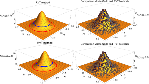
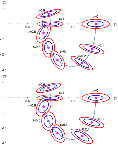
In Figure 1, we have represented the joint 1-PDF of the solution SP of system (27) at t = 0.2 in Cases 1 (top) and 2 (bottom). We can observe that the analytical computations obtained applying RVT method developed in this article agree with Monte Carlo simulations and that the 1-PDF is flattened in the presence of randomness in the model parameters. Similar behavior can be observed considering other times. This issue is better observed in Figure 2, where we have represented the phase portrait. The expectation of the SP solution follows the shape of a spiral line, being represented by a discontinuous curve. This expectation is shown with a pink point at the following times, t = {0, 0.2, 0.4, 0.5, 0.6, 0.9, 1}. Also, at this specific times, confidence regions at 50% and 90% level are plotted in blue and red lines, respectively.

Details are in the caption following the image — **FIGURE 1**
Open in figure viewer PowerPoint

1-PDF of the solution SP to the random oscillator control problem (27). Top: Case 1; bottom: Case 2. Left: By applying RVT method and plotting confidence regions for different confidence level $1 - α$ (blue, $1 - α = 0.5$ and red, $1 - α = 0.9$ ); right: by applying Monte Carlo and RVT method

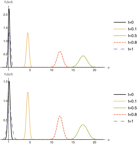
The 1-PDF of control SP, $u (t, ω)$ , for Cases 1 and 2 is shown in Figure 3 at times t = {0, 0.1, 0.5, 0.8, 1}, top and bottom, respectively. We can observe that in both cases it is sharper specially at initial and final times. Notice that the 1-PDFs for a fixed time are more similar when we are at intermediate times.

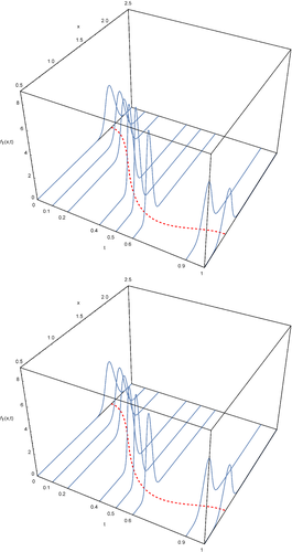
In Figure 4, we have plotted the 1-PDF, f₁(x, t), of the solution SP, $x (t, ω)$ of problem (26), at several times instants in both Cases 1 and 2. Also, the mean $μ_{x} (t)$ has been plotted with red and dashed lines in both cases. Notice that in Case 1 the PDFs are sharper at intermediate times.

5 CONCLUSIONS

In this article, the PDF of a controllable linear system with additive control has been calculated, as well as the PDF of the control in the case that all the coefficients, initial condition and final target are RVs, and the control is a SP. The obtained theoretical results have been applied to study a random damped oscillator. It has been found that by adding more randomness to model parameters, the variability of the solution increases. The results have been validated with Monte Carlo simulations. The equation becomes a system where some of the elements of matrix A are random, which is a novelty with respect to previous works.¹⁰ This is a first step to treat systems in the future where all the elements of A and B are RVs.

ACKNOWLEDGMENTS

This work has been supported by the Spanish Ministerio de Economía, Industria y Competitividad (MINECO), the Agencia Estatal de Investigación (AEI), and Fondo Europeo de Desarrollo Regional (FEDER UE) grant MTM2017-89664-P. Computations have been carried thanks to the collaboration of Raúl San Julián Garcés and Elena López Navarro granted by European Union through the Operational Program of the European Regional Development Fund (ERDF)/European Social Fund (ESF) of the Valencian Community 2014–2020, grants GJIDI/2018/A/009 and GJIDI/2018/A/010, respectively.

CONFLICT OF INTEREST

The authors declare that there is no conflict of interests regarding the publication of this article.

AUTHOR CONTRIBUTIONS

All authors have equally contributed to the whole article.

APPENDIX A: CONSTRUCTION OF THE 1-PDFS IN THE CONTEXT OF THE APPLICATION

In this appendix, we detail how to construct the closed form of both the joint 1-PDF of the solution SP, f₁(y, t), and the 1-PDF of the control SP, f₁(u, t). As in the application we have considered two cases, we obtain the formulas in each scenario.

A.1 Case 1

In this case,

x^{0} (ω) = (x (0, ω), x^{'} (0, ω))

and

x^{1} (ω) = (x (T, ω), x^{'} (T, ω))

are assumed to be independent multivariate normal distributions, while the parameters k and R are considered deterministic quantities. Taking into account that now A is deterministic, we apply expression (22) but only integrating with respect to

x^{0} (ω) = (x (0, ω), x^{'} (0, ω))

. So, in this case, the expression of the joint PDF of the random vector

y (t, ω) = (y_{1} (t, ω), y_{2} (t, ω))

writes

f_{1} (y, t) = \int_{ℝ^{2}} f_{x^{0}} (x^{0}) f_{x^{1}} (M^{- 1} (t, A) y - (M^{- 1} (t, A) - I_{2}) \exp (A t) x^{0}) |\det (M^{- 1} (t, A))| d x_{1}^{0} d x_{2}^{0} .

()

On the other hand, as

x^{0} (ω) \sim N (μ_{0}, \sum_{0})

and

x^{1} (ω) \sim N (μ_{1}, \sum_{1})

where

μ_{1} = (1, 0)

μ_{2} = (2, 0)

, and

\sum_{0}

and

\sum_{1}

are given by (29) and (28), respectively, their density functions are

f_{x^{0}} (x_{1}^{0}, x_{2}^{0}) = \frac{1}{0.0002 π} e^{- \frac{1}{2} ({(\frac{x_{1}^{0} - 2}{\sqrt{0.01}})}^{2} + {(\frac{x_{2}^{0}}{\sqrt{0.01}})}^{2})} and f_{x^{1}} (x_{1}^{1}, x_{2}^{1}) = \frac{1}{0.0001 π} e^{- \frac{1}{2} ({(\frac{x_{1}^{1} - 1}{\sqrt{0.01}})}^{2} + {(\frac{x_{2}^{1}}{\sqrt{0.005}})}^{2})} .

()

Substituting the densities (A2) in the joint 1-PDF indicated in formula (A1), we obtain the closed expression for the joint 1-PDF of the solution SP

y (ω)

. At this point, we notice that we have carried out computations by Mathematica^© software, and it allows us to define f₁(y, t) as an integral. Matrix M(t, A) in (A1) can be computed from formulas (14)–(17). Analogously, the 1-PDF of the control SP can be calculated. In this case, from the expression (25) taking into account again that A is deterministic, one gets

f_{1} (u, t) = \int_{ℝ^{3}} f_{x^{0}} (x^{0}) f_{x^{1}} (J {(t, A)}^{- 1} (u + J (t, A) e^{A T} x^{0})) |\det J {(T, A)}^{- 1}| d x_{1}^{0} d x_{2}^{0} d x_{2}^{1},

()

where

J (t, A) = q^{⊤} (t, A) Λ^{- 1} (T, A)

with matrices q and

Λ

given in (14) and (15), respectively. Note that, all the matrices,

Λ (t, A)

, q(t, A), V(t, A), M(t, A), and J(t, A) have been directly symbolically defined in Mathematica^©. Although, final expressions for matrices M(t, A) and J(t, A), and their corresponding inverses, can be calculated, its expressions are very cumbersome. Then, we define them using the commands NIntegrate, MatrixExp, and Inverse, among others.

A.2 Case 2

In this case,

x^{0} (ω) = (x (0, ω), x^{'} (0, ω))

x^{1} (ω) = (x (T, ω), x^{'} (T, ω))

k (ω)

, and

R (ω)

are assumed to be independent and following normal distributions. Now the expression of the joint 1-PDF of the random vector

y (ω) = (y_{1} (ω), y_{2} (ω))

f_{1} (y, t) = \int_{ℝ^{4}} f_{x^{0}} (x^{0}) f_{x^{1}} (M^{- 1} (t, A) y - (M^{- 1} (t, A) - I_{2}) \exp (A t) x^{0}) f_{k} (k) f_{R} (r) |\det (M^{- 1} (t, A))| d x_{1}^{0} d x_{2}^{0} d k d r .

()

The densities of

x^{0} (ω)

and

x^{1} (ω)

are calculated in (A2). With respect to RVs

k (ω)

and

R (ω)

, they have truncated normal distributions. Then, we are able to calculate expressions for both densities

f_{k} (k) = \{\begin{cases} 1.99471 e^{- 12.5 {(k - 10)}^{2}}, & 9 < k \leq 11, \\ 0, & o t h e r w i s e, \end{cases} and f_{R} (r) = \{\begin{cases} 3.98943 e^{- 50 {(r - 1)}^{2}}, & 0.5 < r \leq 1.5, \\ 0, & o t h e r w i s e . \end{cases}

()

Substituting the densities indicated in (A2) and (A5) in the joint 1-PDF given by formula (A4), we obtain the closed expression for the joint 1-PDF of the solution SP

y (t, ω)

. As in the previous case, all calculations in these scenario have been carried out using Mathematica^© software defining the matrices symbolically.

Biographies

Juan-Carlos Cortés is a Full Professor of Applied Mathematics at Universitat Politècnica de València (UPV). He develops his research in Mathematical Modeling with Uncertainty in the Instituto Universitario de Matemática Multidisciplinar at the UPV.
Ana Navarro-Quiles is an Assistant Professor at Universitat de València. Her research focuses on the study, from a probabilistic point of view, of random differential equations as well as their applications.
José-Vicente Romero is an Associate Professor of Applied Mathematics at Universitat Politècnica de València (UPV). His investigation deals with Stochastic Problems and Applications in the Instituto Universitario de Matemática Multidisciplinar at the UPV.
María-Dolores Roselló is an Associate Professor of Applied Mathematics at Universitat Politècnica de València (UPV). Her research focuses on Random Systems and Applications in the Instituto Universitario de Matemática Multidisciplinar at the UPV.

REFERENCES

1Zabczyk J. Mathematical Control Theory: An Introduction. Modern Birkhäuser Classics. Boston, MA: Birkhäuser; 2008.
10.1007/978-0-8176-4733-9
Google Scholar
2Dorf RC, Bishop RH. Modern Control Systems. 9th ed. Upper Saddle River, NJ: Prentice-Hall, Inc; 2000.
Google Scholar
3Nise NS. Control Systems Engineering. 3rd ed. Hoboken, NJ: John Wiley & Sons, Inc; 2000.
Web of Science® Google Scholar
4Bavafa-Toosi Y. Introduction to Linear Control Systems. Amsterdam, Netherlands: Elsevier Science; 2017.
Google Scholar
5Shaikhet L. Improved condition for stabilization of controlled inverted pendulum under stochastic perturbations. Discrete Contin Dyn Syst. 2009; 24(4): 1335-1343. https://doi.org/10.3934/dcds.2009.24.1335.
10.3934/dcds.2009.24.1335
Web of Science® Google Scholar
6Dragan V, Aberkane S, Popa IL. Optimal H² filtering for periodic linear stochastic systems with multiplicative white noise perturbations and sampled measurements. J Franklin Inst. 2015; 352(12): 985-6010. https://doi.org/10.1016/j.jfranklin.015.10.010.
10.1016/j.jfranklin.2015.10.010
Web of Science® Google Scholar
7Li X, Song S. Research on synchronization of chaotic delayed neural networks with stochastic perturbation using impulsive control method. Commun Nonlinear Sci Numer Simul. 2014; 19(10): 3892-3900. https://doi.org/10.1016/j.cnsns.2013.12.012.
10.1016/j.cnsns.2013.12.012
Web of Science® Google Scholar
8Liu S, Debbouche A, Wang J. On the iterative learning control for stochastic impulsive differential equations with randomly varying trial lengths. J Comput Appl Math. 2017; 312: 47-57. https://doi.org/10.1016/j.cam.2015.10.028.
10.1016/j.cam.2015.10.028
Web of Science® Google Scholar
9Soong TT. Random Differential Equations in Science and Engineering. New York, NY: Academic Press; 1973.
Google Scholar
10Cortés JC, Navarro-Quiles A, Romero JV, Roselló MD, Zuazua E. Full probabilistic solution of a finite dimensional linear control system with random initial and final conditions. J Franklin Inst. 2020; 357(12): 8156-8180. https://doi.org/10.1016/j.jfranklin.2020.06.005.
10.1016/j.jfranklin.2020.06.005
Web of Science® Google Scholar
11Levine J. Analysis and Control of Nonlinear Systems. Berlin/Heidelberg: Springer; 2009.
10.1007/978-3-642-00839-9
Google Scholar
12Lazar M, Zuazua E. Greedy controllability of finite dimensional linear systems. Automatica. 2016; 74: 327-340. https://doi.org/10.1016/j.automatica.2016.08.010.
10.1016/j.automatica.2016.08.010
Web of Science® Google Scholar

Citing Literature

All articles

Solving fully randomized higher-order linear control differential equations: Application to study the dynamics of an oscillator

Abstract

1 INTRODUCTION

2 CONTROLLABLE RANDOMIZED EQUATION

3 COMPUTATION OF THE 1-PDF OF SOME STOCHASTIC PROCESSES OF INTEREST IN CONTROL PROBLEMS

3.1 Computing the 1-PDF of the solution SP

3.2 Computing the 1-PDF of the control SP

4 APPLICATION TO STUDY THE DYNAMICS OF A RANDOM OSCILLATOR

5 CONCLUSIONS

ACKNOWLEDGMENTS

CONFLICT OF INTEREST

AUTHOR CONTRIBUTIONS

APPENDIX A: CONSTRUCTION OF THE 1-PDFS IN THE CONTEXT OF THE APPLICATION

A.1 Case 1

A.2 Case 2

Biographies

REFERENCES

Citing Literature

Figures

References

Information

About Wiley Online Library

Help & Support

Opportunities

Connect with Wiley

Solving fully randomized higher-order linear control differential equations: Application to study the dynamics of an oscillator

Abstract

1 INTRODUCTION

2 CONTROLLABLE RANDOMIZED EQUATION

3 COMPUTATION OF THE 1-PDF OF SOME STOCHASTIC PROCESSES OF INTEREST IN CONTROL PROBLEMS

3.1 Computing the 1-PDF of the solution SP

3.2 Computing the 1-PDF of the control SP

4 APPLICATION TO STUDY THE DYNAMICS OF A RANDOM OSCILLATOR

5 CONCLUSIONS

ACKNOWLEDGMENTS

CONFLICT OF INTEREST

AUTHOR CONTRIBUTIONS

APPENDIX A: CONSTRUCTION OF THE 1-PDFS IN THE CONTEXT OF THE APPLICATION

A.1 Case 1

A.2 Case 2

Biographies

REFERENCES

Citing Literature

Figures

References

Related

Information