Volume 3, Issue 4 e1156
RESEARCH ARTICLE
Full Access

The classic two-player gambler's ruin problem with successive events: A generalized variance

Abid Hussain

Corresponding Author

Abid Hussain

Department of Statistics, Govt. College Khayaban-e-sir syed, Rawalpindi, Pakistan

Correspondence Abid Hussain, Department of Statistics, Govt. College Khayaban-e-sir syed, Rawalpindi, Pakistan.

Email: [email protected]

Search for more papers by this author
Salman A. Cheema

Salman A. Cheema

Department of Applied Sciences, National Textile University, Faisalabad, Pakistan

Search for more papers by this author
First published: 12 March 2021
Citations: 1

Abstract

In this article, we present the general expressions for the variance of the ruin time of the classic two-player gambler's ruin problem with successive and nonoverlapping trials. The rationale of this game plan is motivated by its exhibition in the game of tennis, where a player is required to win two consecutive serves to win the point after achieving deuce. This strategy (i.e., decision is based on successive and nonoverlapping trials) is in favor of the player, who plays with a better skill set and reduces the chances of decision based only on luck. We explicitly derive the general expressions of variance up to m successive and non-overlapping trials for the case of symmetric and asymmetric games. It is proved that the expressions given in literature for the symmetric and asymmetric cases are the sub cases of our proposed expressions. Finally, some special games (i.e., m = 2) are simulated and the results are verified with the proposed formulas.

1 INTRODUCTION

In classic version of the ruin problem, two players initiate with x and t − x stakes, say dollars, involved in the game. Here, x is the initial stake of the gambler and t denotes the total stake involved in the game. After a trial, the gambler wins with probability p and losses with probability q, where p + q = 1. This problem was, probably, first posed by Pascal, see for example, Reference 1 for a historical background. Since then, a variety of associated questions, game modifications, and extensions have been considered in the literature. For example, for the expressions of ruin probability and ruin time of the game, see Reference 2. Further, the conditional expectations of the ruin time of game, were investigated in References 3-5. Where, Reference 6 proposed the use of tie event and thus insisted on more realistic version of the classic problem. More recently, in adjacent past Reference 7, yet introduced another variant of the classic ruin problem by involving occurrence of successive events in the decision-making process.

Over the time, a consistent interest of the experts investigating the variance structures of the ruin problem and related amendments, can be witnessed. For example, Reference 8 provided the results for higher conditional moments for the classic problem. In next phase, Reference 9 calculated the expression of the classic two-player game. However, his work remained of limited utility, as it was only applicable for symmetric game when even number of total fortune is involved in the game. The variance expression is of the following form:
v ( T ) = x ( t x ) 3 ( x 2 + ( t x ) 2 2 ) , ()
where T be the remaining trials to terminate the game. Further, Reference 10 provided a comprehensive set of expressions for the two-player gambler's ruin problem with ties, dealing with symmetric and asymmetric games. The expression for the symmetric game is given as:
v ( T ) = x ( t x ) 12 p 2 ( x 2 + ( t x ) 2 + 1 6 p ) , ()
where the variance of asymmetric game is calculated as:
v ( T ) = t 2 r 2 x p 2 ( r 1 ) 2 ( r t 1 ) 2 + 4 t r x x p 2 ( r 1 ) 2 ( r t 1 ) + t r x ( ( p ( r 1 ) 2 r 1 ) ( r t 1 ) t ( r 1 ) ( 3 r t 1 ) ) p 2 ( r 1 ) 3 ( r t 1 ) 2 x ( p ( r 1 ) 2 r 1 ) p 2 ( r 1 ) 3 + t ( ( 1 3 t ) r t + ( 1 + 3 t ) r t + 1 p ( r 1 ) 2 ( r t 1 ) r 1 ) p 2 ( r 1 ) 3 ( r t 1 ) 2 , ()
where r = q/p. The above expression is valid for both cases, that is, the ties are involved if p + q < 1 and when no involvement of tie, p + q = 1.
This article aims at calculating the variance expressions for the most recent development proposed by Reference 7 in the literature of ruin problem. They devised a novel strategy of involving the occurrence of m number of successive and nonoverlapping events in the decision-making process. The proposed scheme was shown to be advantageous on two fronts, (i) both players have increased number of games to play but with lesser chances of developing stalemate, and (ii) the decision process favors the player with a better skill set and thus reduced the likelihood of win or loss based only on luck.7 provided the expressions of ruin probability (Px), ruin time (E(T)) and conditional ruin times of the game, that is, Ex (the expected duration when gambler loses the game) and Fx (the expected duration when gambler wins the game). The formulas are given as under:
P x = t x t ; q = p ( r m ) x ( r m ) t 1 ( r m ) t ; q p , E ( T ) = m 2 m 1 x ( t x ) ; q = p m q m p m ( t ( ( r m ) x 1 ) 1 ( r m ) t + x ) ; q p , E x = m 2 m 1 x 3 ( 2 t x ) ; q = p m ( p m q m ) 1 ( r m ) x ( r m ) t ( x ( ( r m ) x + ( r m ) t ) + 2 t ( ( r m ) x + t ( r m ) t 1 ( r m ) t ) ) ; q p ,
and
F x = m 2 m 1 3 ( t 2 x 2 ) ; q = p m ( p m q m ) 1 1 ( r m ) x ( ( t x ) ( ( r m ) x + 1 ) + 2 t ( ( r m ) x ( r m ) t ( r m ) t 1 ) ) ; q p .

In upcoming Section 2, we present the mathematical structures obtaining the variance expressions under Reference 7 proposed strategy of successive events. In next section (Section 3), we evaluate the validity of mathematical findings of Section 2, both numerically and through simulation-based investigation. Finally, we summarize our research in Section 4.

2 MATHEMATICAL DERIVATIONS

For the ruin time, let T be the remaining trials to terminate the game. We define,
D x = E ( T ) = n = 0 n P ( n | x ) ,
where, P(n|x) is a probability function and must satisfy: n = 0 P ( n | x ) = 1 and,
H x = E ( T 2 ) = n = 0 n 2 P ( n | x ) .
The Dx can be calculated for two successive and nonoverlapping events, that is, m = 2 (and then we have provided all the general expressions for any value of m at the end of each derived formula) by using the law of total expectation, such as:
D x = p 2 ( 2 + D x + 1 ) + 2 p q ( 2 + D x ) + q 2 ( 2 + D x 1 ) , p 2 D x + 1 ( 1 2 p q ) D x + q 2 D x 1 = 2 . ()
Similarly,
H x = p 2 ( H x + 1 + 4 D x + 1 + 4 ) + 2 p q ( H x + 2 + 4 D x + 4 ) + q 2 ( H x 1 + 4 D x 1 + 4 ) , p 2 H x + 1 ( 1 2 p q ) H x + q 2 H x 1 = 4 p 2 D x + 1 8 p q D x 4 q 2 D x 1 4 .
After inserting Equation (4) into the above equation, we get the following equation:
p 2 H x + 1 ( 1 2 p q ) H x + q 2 H x 1 = 4 ( 1 D x ) . ()
As, our interest lies in the calculation of the variance expression for the desired game plan, such as:
v ( T ) = H x D x 2 .

Therefore, we are required to find the solutions for the difference equations (4) and (5). The objectives are attained through the method of undetermined coefficients. In the upcoming subsections, we treat the symmetric case, that is, p = q = 1/2 and asymmetric case, where p ≠ q, separately.

2.1 The variance for the case of symmetry

For the general solution of Equation (4),7 derived the following expression for the ruin time, when p = q = 1/2, such as:
D x = 4 x ( t x ) . ()
By using Equation (6) into Equation (5), we get the following expression,
H x + 1 2 H x + H x 1 = 16 64 t x + 64 x 2 . ()
The characteristic equation results in one double root, that is, λ 1 = λ 2 = 1 , and the complementary solution, such as Hx = A1 + A2x. Afterward, we search for a particular solution in the form of Hx = A3x2 + A4x3 + A5x4. By imposing the particular solution in the equation (7), we obtain A3 = 8/3, A4 = −32t/3 and A5 = 16/3. Hence the general solution for Equation (7) takes the following form:
H x = A 1 + A 2 x + 8 3 x 2 32 3 t x 3 + 16 3 x 4 .
After employing the two boundary conditions, that is,s H0 = Ht = 0, we get the following solution,
H x = 8 3 ( 2 t 2 1 ) t x + 8 3 x 2 32 3 t x 3 + 16 3 x 4 . ()
Since, v ( T ) = H x D x 2 , therefore,
v ( T ) = 4 x ( t x ) 3 ( 4 x 2 + 4 ( t x ) 2 2 ) . ()
Let us say, t = x + y, then the above expression is written in a “more symmetric” form:
v ( T ) = 4 x y 3 ( 4 x 2 + 4 y 2 2 ) . ()
Now, we study the initial fortunes x, y, maximizing the variance (v(T) = v(x)) for fixed t = x + y > 0 and p = q = 1/2. Consider the first case of even t, that is, t = 2n for some n . Then
v ( x ) = v ( 2 n x ) ,
and,
v ( n ) v ( n k ) = 4 3 k 2 ( 8 k 2 2 ) ,
where, k = 1, 2, … , n. It holds the inequalities in the form of
v ( n ) > v ( n 1 ) > v ( n 2 ) > .
Note that, in a simple game with no ties, the v(x) takes the form of
v ( n ) = v ( n 1 ) > v ( n 2 ) > ,
which is consistent with Reference 10.
Next, we consider the second case, that is, the total fortune involved in the game, is odd, such as t = 2n + 1 for some n . Then, v(x) = v(2n + 1 − x), and we have v(n + 1) = v(n). Thus, we get the following equality,
v ( n ) v ( n k ) = 8 3 k ( 4 k 3 + 8 k 2 + 5 k + 1 ) ,
where, k = 1, 2, … , n. This maintains the inequalities in the form of v(n) > v(n − 1) > v(n − 2) > …. One may notice that, for the symmetric game, the maximum value of the variance is observed when |x − y| equals to zero or one, only.
We can generalize the expression given in equation (10) for any number of successive and nonoverlapping events, that is,s m, as:
v ( T ) = m 2 m 1 x y 3 ( m 2 m 1 x 2 + m 2 m 1 y 2 2 ) . ()

It remains verifiable, that for m = 1, the above expression reduces to Reference 9, given in Equation (1).

2.2 The variance for the case of asymmetry

Now, let us consider the case of p ≠ q. For the general solution of Equation (4), Reference 7 derived the following expression:
D x = 2 q 2 p 2 ( t ( ( r 2 ) x 1 ) 1 ( r 2 ) t + x ) , ()
where, r = q p . It is trivial to verify that, lim p q D x = 4 x ( t x ) . Thus,
D x = lim p q 2 t ( ( q 2 p 2 ) x 1 ) 2 x ( ( q 2 p 2 ) t 1 ) ( p 2 q 2 ) ( ( q 2 p 2 ) t 1 ) ,
which results into an undetermined form of 0 0 . After using the L. Hospital rule, we get the following form:
D x = lim p q 4 x t q 2 x p 2 x 1 + 4 x t q 2 t p 2 t 1 2 p ( q 2 t p 2 t 1 ) ( p 2 q 2 ) ( 2 t q 2 t p 2 t 1 ) .

After an other iteration of L. Hospital rule, we obtained D x = x ( t x ) q 2 . One may notice that, for q = 1/2, the resultant Dx remains similar to that of Equation (6).

Now, if we consider Dx as a function of a continuous variable x then it is easy to show that the second derivative, d 2 D x d x 2 , is negative ∀ x, and thus the function Dx is strictly concave with a maximum attained at the point:
x = log ( r 2 t 1 t log ( r 2 ) ) [ log ( r 2 ) ] 1 ,
where x depends on two values, i.e. total stake, t, involved in the game and the ratio r = q/p.
For the variance of ruin time, we impose Equation (12) into Equation (5), and get the following equation.
p 2 H x + 1 ( 1 2 p q ) H x + q 2 H x 1 = ( 4 8 t s ( 1 r 2 t ) ) + ( 8 s ) x + ( 8 t s ( 1 r 2 t ) ) r 2 x , ()
where s = p2 − q2. The characteristic equation gives two different roots, that is, λ 1 = 1 and λ 2 = q 2 p 2 = r 2 , therefore the complementary solution is the form of Hx = B1 + B2(r2)x. Afterward, we search for a particular solution in the form of Hx = B3x + B4x2 + B5x(r2)x. By imposing this in Equation (13), we obtained the following results:
B 3 = 4 s 2 ( 1 r 2 t ) 8 s t 4 ( p 2 + q 2 ) ( 1 r 2 t ) s 3 ( 1 r 2 t ) , B 4 = 4 s 2 ,
and,
B 5 = 8 t s 2 ( 1 r 2 t ) .
Hence the general solution of Equation (13), will be in the following form:
H x = B 1 + B 2 ( r 2 ) x + B 3 x + B 4 x 2 + B 5 x ( r 2 ) x . ()
By using the two boundary conditions, that is, H0 = Ht = 0, we further obtain:
B 1 = 8 t 2 ( 1 + r 2 t ) s 2 ( 1 r 2 t ) 2 4 t ( s 2 + s t p 2 q 2 ) s 3 ( 1 r 2 t ) ,
and,
B 2 = 4 t ( s 2 + s t p 2 q 2 ) s 3 ( 1 r 2 t ) 8 t 2 ( 1 + r 2 t ) s 2 ( 1 r 2 t ) 2 .
Finally, we have
v ( T ) = B 1 + B 2 ( r 2 ) x + B 3 x + B 4 x 2 + B 5 x ( r 2 ) x D x 2 . v ( T ) = 8 t 2 ( 1 + r 2 t ) s 2 ( 1 r 2 t ) 2 4 t ( s 2 + s t p 2 q 2 ) s 3 ( 1 r 2 t ) + 4 t ( s 2 + s t p 2 q 2 ) s 3 ( 1 r 2 t ) r 2 x 8 t 2 ( 1 + r 2 t ) s 2 ( 1 r 2 t ) 2 r 2 x + 4 s 2 ( 1 r 2 t ) 8 s t 4 ( p 2 + q 2 ) ( 1 r 2 t ) s 3 ( 1 r 2 t ) x + 4 s 2 x 2 8 t s 2 ( 1 r 2 t ) x r 2 x 2 t ( 1 r 2 x ) s ( 1 r 2 t ) 2 x s 2 ,
which simplify as the following expression:
v ( T ) = 4 t 2 ( 1 ( r 2 ) 2 x ) + 8 t 2 ( r 2 ) t ( 1 ( r 2 ) x ) s 2 ( 1 ( r 2 ) t ) 2 + 4 x ( s 2 p 2 q 2 ) s 3 + 4 t ( s 2 + s t p 2 q 2 ) ( ( r 2 ) x 1 ) s 3 ( 1 ( r 2 ) t ) 16 x t ( r 2 ) x s 2 ( 1 ( r 2 ) t ) . ()
The generalization of the expression given in Equation (15), for any number of successive and nonoverlapping events, that is, m, is given as:
v ( T ) = m 2 m 1 t 2 ( 1 ( r m ) 2 x ) + 2 m 2 m 1 t 2 ( r m ) t ( 1 ( r m ) x ) s 2 ( 1 ( r m ) t ) 2 + m 2 m 1 x ( s 2 p m q m ) s 3 + m 2 m 1 t ( s 2 + s t p m q m ) ( ( r m ) x 1 ) s 3 ( 1 ( r m ) t ) 4 m 2 m 1 x t ( r m ) x s 2 ( 1 ( r m ) t ) ,
where s = pm − qm. One can easily verify that, for m = 1, the above expression is of the form derived by Reference 10, given in Equation (3), for both cases when no ties are involved in the game, that is, p + q = 1 and the ties are involved, that is, p + q < 1.

3 PERFORMANCE EVALUATION

3.1 Numerical results

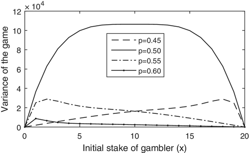
Table 1 presents the values of v(T), for both symmetric and asymmetric games. The variance behavior is then quantified under various parametric settings while fixing the more practical and feasible value of nonoverlapping and successive events, that is, m = 2. Moreover, for the demonstration purposes we considered, t = 20 and x = 5, 10, and 15. For the case of symmetric game, we notice that the variance gains its maximum value at x = t/2 = 10, where x ∈ (0, t). For the asymmetric game, the above settings are further studied for the variant value of winning probabilities of the gambler, such as p = 0.20 to p = 0.90. It is observable that the x depends only, on the total fortune in game, that is, t and on the ratio q2/p2. Further exploration of the particular setting indicates that the function v(T) has a maxima attained at point x, such that x ∈ (0, t/2) if q < p and x ∈ (t/2, t) if q > p. For visual demonstration purposes, the graphs of v(T) are depicted in Figure 1, as functions of continuous variable of initial dollar, that is, x. Display behaviors of variability with respect to winning probability and initial stake, stay consistent with the theoretical and mathematical orientation of the strategy.
Details are in the caption following the image
The variance of ruin time for t = 20 and a sample of probabilities p
TABLE 1. The variance of the ruin time for m = 2 with t = 20, along 50,000 simulations
p x y = t − x v(T) Simulations
5 15 29.63 29.1036
0.20 10 10 59.26 59.0589
15 5 88.89 90.3146
5 15 60.00 58.5949
0.25 10 10 120.00 118.9178
15 5 180.00 179.4343
5 15 131.25 131.7653
0.30 10 10 262.50 264.3643
15 5 393.64 392.4603
5 15 9194.71 9136.837
0.45 10 10 16,307.35 16,273.20
15 5 21,637.20 22,052.30
5 15 99800 100,254.50
0.50 10 10 106,400 106,486.50
15 5 99,800 100,131.44
5 15 3504.74 3533.9530
0.60 10 10 2386.56 2383.4180
15 5 1199.57 1204.4470
5 15 1008.27 1009.3200
0.65 10 10 673.99 665.8152
15 5 337.04 336.8547
5 15 44.61 44.8808
0.85 10 10 29.74 29.6462
15 5 14.87 15.1053
5 15 21.09 21.0858
0.90 10 10 14.06 14.1915
15 5 7.03 7.1249

3.2 Simulation study

In this subsection, we validate the numerical findings of the Section 3.1, through a rigorous simulation study. The games involving m = 2 are simulated with MATLAB (version R2015a). The reported results are based on 50,000 execution of games, for symmetric and asymmetric cases. A vividly close match between numerical results and simulated findings remains motivational.

4 SUMMARY AND FUTURE WORK

In this paper, we provided the expressions of the variance of the classic two-player ruin's problem based on successive events. The mathematical results are established for both, symmetric and asymmetric games, involving even and odd dollars as total stake in the game. This research extends the existing ruin problem literature for a novel strategy minimizing the extent of indecisiveness in the game and weighing the skill set of players, heavily. In future, it is attractive to investigate the variability structure for the game involving three players.

ACKNOWLEDGEMENTS

The authors are very grateful to the chief-in-editor and referees for their valuable suggestions that have made this article worthy to be published.

    CONFLICTS OF INTEREST

    No conflict of interest is reported by authors.

    Biographies

    • biography image

      Dr. Abid Hussain obtained his PhD (Statistics) degree in 2018 from Quaid-i-Azam University, Islamabad, Pakistan. His focused research areas of interest are Applied Probability, Stochastic Processes, Operations Research and Nonparametric Statistics.

    • biography image

      Dr. Salman A.Cheema obtained his PhD Statistics degree from The University of Newcastle, Australia and MS Statistics degree from Virginia Tech, USA. His focused research areas include Data masking, Optimization, Choice Models and Social desirability bias.

      The full text of this article hosted at iucr.org is unavailable due to technical difficulties.