We describe a method for computing the number of Hamilton cycles in cubic polyhedral graphs. The Hamilton cycle counts are expressed in terms of a finite-state machine, and can be written as a matrix expression. In the special case of polyhedral graphs with repeating layers, the state machines become cyclic, greatly simplifying the expression for the exact Hamilton cycle counts, and let us calculate the exact Hamilton cycle counts for infinite series of graphs that are generated by repeating the layers. For some series, these reduce to closed form expressions, valid for the entire infinite series. When this is not possible, evaluating the number of Hamiltonian cycles admitted by the series' k-layer member is found by computing a (k − 1)^th matrix power, requiring $𝒪 (\log_{2} (k))$ matrix-matrix multiplications. We demonstrate our technique for the two infinite series of fullerene nanotubes with the smallest caps. In addition to exact closed form and matrix expressions, we provide approximate exponential formulas for the number of Hamilton cycles.

1 Introduction

A Hamilton cycle is a spanning cycle in a graph $G = (𝒱, ℰ)$ , that is, a closed path that visits every vertex exactly once. In general, determining whether a given graph has at least one Hamilton cycle is NP-complete, including for cubic polyhedral graphs.^1-3 Thus, counting all Hamilton cycles is #P-complete, the complexity class for counting solutions to NP-complete problems: a computationally much harder problem.^{4, 5} Figure 1 shows the most famous example of a cubic polyhedral graph that does not admit a Hamilton cycle. For a history of Hamiltonian graphs, see Wilson.⁶

Details are in the caption following the image — **FIGURE 1**
Open in figure viewer PowerPoint

The Tutte graph ((A) a planar drawing of the graph, and (B) a 3D embedding produced using the software in References 7 and 8) is an example of a cubic polyhedral graph that is not Hamiltonian. In general, determining whether a given polyhedral graph admits a Hamilton cycle is an NP-complete problem, whereby counting the number of Hamilton cycles is a #P-complete problem

Within the class of cubic polyhedral graphs, there is at least one subclass of layered cubic planar graphs, defined by Franzblau, which are always Hamiltonian.⁹ Those are graphs that can be completely decomposed into—not necessarily identical—concentric cycles, where neighboring cycles are connected by two or more edges and where the first and last cycles are identical to a face.

In the special case of layered graphs that are the underlying graphs of closed nanotubes (a subclass of fullerenes), we can decompose the graph into layers, such that a sequence of layers is identical and consists only of hexagons. These identical layers are characterized by the chiral vectors C_h = (n, m).

Since layered cubic planar graphs are always Hamiltonian, counting their Hamiltonian cycles is no longer #P-complete, opening for the possibility of discovering more efficient algorithms.

In the following (Section 2), we first describe a method for counting Hamilton cycles in any cubic polyhedral graph. This method is applied to the special case of layered polyhedral graphs, for which it efficiently computes the number of Hamilton cycles. The method works not just for single graphs, but applies to infinite inductively defined series, yielding exact closed form expressions in simple cases, and expressions in terms of matrix powers for more difficult cases. In Section 3, we demonstrate it on the two infinite series of layered fullerene graphs with the smallest caps. A proof for the main theorem, showing that the method indeed produces exact Hamilton cycle counts, is given in Section 4.

2 Counting Hamilton cycles in a cubic polyhedral graph

We introduce here a general technique for counting the Hamilton cycles in cubic polyhedral graphs. As the general problem is #P complete, it will in the fully general case require exponential time in the graph size, as it must. However, for layered graphs of bounded layer size, it reduces down to polynomial time. While we begin by describing how the method works for a single polyhedral graph, the method's strength—and the motivation for us to introduce it—is for finding exact expressions for the Hamiltonian cycle count for entire infinite series of layered polyhedral graphs.

We begin by identifying Hamilton cycles with certain bi-colorings. Figure 2 illustrates this correspondence. While this identification has been used before for layered graphs,^{9, 10} we make it precise and prove its correctness for all cubic polyhedral graphs.

Lemma 1. (Hamiltonian cycles as bi-colorings)Given a cubic polyhedral graph G, and a choice of one of its faces F₀, there is a bijection between the set of Hamilton cycles and the set of face bi-colorings on G that have the following three properties: (a) F₀ is unshaded, (b) Every vertex is adjacent to at least one shaded and one unshaded face, and (c) all shaded and all unshaded faces are connected.

Proof.Let there be given a cubic polyhedral graph G and a choice for F₀ (which will be the “outer face” in the planar drawings used to illustrate the method), and consider a Hamiltonian cycle $γ$ on G. By Jordan's curve theorem, $γ$ separates the surface uniquely into two connected regions, since it traces a simple closed curve on G's surface. Let the entire region containing F₀ be white (without loss of generality), and the other region shaded. Hamiltonicity implies that every vertex of G must lie on the boundary between the shaded and unshaded region. Hence, this bi-coloring fulfills properties (a), (b), and (c). It is unique since the color of F₀ is fixed, whereby it yields a well-defined mapping f from the Hamilton cycles to the set of colorings that fulfill (a), (b), and (c). Finally, the edges comprising the Hamilton cycle are the boundary between the two regions, any two distinct cycles yield distinct colorings, whereby f is injective.

Conversely, let there be given a bi-coloring of G's faces fulfilling properties (a), (b), and (c). By property (c), the edge set comprising the boundary forms a simple cycle $γ$ , which by property (b) visits every vertex in G, that is, it is a Hamilton cycle. Hence, this bi-coloring is the value $f (γ)$ , whereby f is also surjective.

In all, f is bijective, so we can identify the Hamiltonian cycles through f with the bi-colorings that fix the color of F₀ and fulfill (b) and (c).

Definition 1. (Cap)A cap is a subgraph that has exactly one boundary. It must have at least one face and no leafs.

Definition 2. (Layer)A layer is a subgraph that has exactly two boundaries which do not have any vertices in common. It may not have any leafs. That is, it has exactly two holes with respect to the parent graph.

For a polyhedral graph, exactly two caps can be defined, corresponding to two opposite ends of the polyhedron. The caps are not uniquely defined, however, but can be chosen in many ways, as can the subdivision of the remaining graph into layers between the two caps. In the following, we consider a polyhedral graph G and assume that this choice has been made, such that G is composed of a start-cap A, an end-cap Z, and in between them: k layers. Each layer has an inner and an outer boundary cycle. If k = 1, the outer boundary is the boundary of A, and the inner cycle is the boundary of Z. If k ≥ 2, the two terminal layers share a boundary with A and Z, respectively, and for 1 ≤ i < k, the inner boundary of layer i is the outer boundary of layer i + 1.

We write S ⊕ T for the combined graph of subgraphs S and T, merged by identifying the inner boundary of S with the outer boundary of T. A and Z only have one boundary each, respectively considered “inner” and “outer.”

Consider now a polyhedral graph that is partitioned into two caps and zero or more layers. We do not address here the question of how to optimally decompose a graph into caps and layers.

The second important step needed to construct the Hamilton cycle counting method is the following locality condition, which ensures that we can count incrementally by way of a finite state-machine. We start from one cap and end in the other:

Lemma 2. (Locality)When shading in a graph which is decomposed into layers according to the rules defined in Lemma 1, the legal colorings of each layer depend only on the previous layer and which of the shaded and unshaded faces in the previous layer are already connected, that is, which shaded faces in the previous layer are connected by shaded faces in the subgraph that consists of all previous layers and the starting cap (and respectively for unshaded faces).

Proof.By Lemma 1(c), for a shading of faces to correspond to a Hamilton cycle, it is required that all shaded and all unshaded faces, respectively, are connected after all faces are colored in.

During the process of shading in the graph layer-wise, the set of shaded faces may temporarily be disconnected. However, in order to connect them through the following layers, each shaded face must through other shaded faces be connected to the boundary where new layers are added. This analogously applies to unshaded faces.

In order to fulfil this requirement, we must include information on the connectedness of shaded faces into a local layer description.

Lemma 1 requires that each vertex is adjacent to a shaded and an unshaded face. As all vertices in a graph that is decomposed into layers are either interior to the layer or lie on the boundary between one layer and the next, the face adjacency of each vertex is fully determined by the two layers and their orientation and does not depend on any other layers.

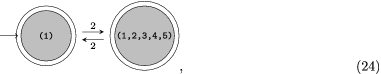
Because of the locality condition of Lemma 2, we can model the counting as a finite state machine, in which the finitely many states are the legal shadings of single layers together with the information about which shaded faces are connected. We represent the state machine as a directed multigraph M, in which the edges represent transitions to states that are accessible from the corresponding state. The directed subgraph that describes the transition from one layer to the following one is denoted as M^(p). If one state can be followed by another state in more than one way (due to symmetry), they are connected by multiple directed edges. We call the vertices that correspond to starting points initial states (typically every valid shading of the first cap), and those that can be final layers in a Hamilton cycle accepting states(typically every valid shading of the last cap).

The number of Hamilton cycles admitted by a graph that consists of two caps and k layers is then the number of paths of length k + 1 in M that originate in an initial state (start-cap bi-coloring) and end in an accepting state (end-cap bi-coloring). See Figure 3(B).

The state-machine can equivalently be represented by a very sparse square matrix M, with M_st = n if $s \to_{}^{n} t$ is an arc of M, and M_st = 0 otherwise. In the k^th power of M, the entry $M_{s t}^{k}$ is the number of length-k paths from state s to state t. Hence, the number of Hamilton cycles can be counted by raising M to the k^th power and summing the elements of the AZ-subblock, consisting of the initial-state rows and final-state columns. This sum is the number of Hamilton cycles.

M is zero everywhere except in the blocks M^(p) directly above the diagonal, representing the directed subgraphs M^(p) : L_p → L_p + 1 that link layer p to layer p + 1, as shown in Figure 3(C) (where we identify A = L₀ and Z = L_k + 1). The small blocks M^(p) are still sparse, but rectangular with dimensions N_p × N_p + 1, where N_p is the number of valid shadings for layer p (with A and Z as p = 0 and p = k + 1).

Because of this, we can calculate the number of Hamilton cycles as a single length-(k + 1) product of the much smaller blocks M^(p). The entry M^(p)_st in the adjacency matrix is the number of single-step transitions from state s in layer p to state t in layer (p + 1). In the product of two consecutive matrices M^(p) and M^(p + 1), the entry (s, t) is the number of length-2 paths from state s in layer p to state t in layer (p + 2), and so forth. The product of the k + 1 matrices M^(p) directly yields the AZ-subblock of M^k, and thus sums to the number of Hamilton cycles. This representation makes calculations convenient, shown in Equations (1) and (3) below.

2.1 An acyclic finite state-machine that counts Hamilton cycles in polyhedral graphs

We are now ready to construct a finite state machine that counts the Hamiltonian cycles in infinite series of cubic layered-graphs.

The following procedure constructs a deterministic finite automaton (DFA), such that paths of length k + 1 starting in an initial state and ending in a final state count the number of Hamilton cycles in G_k:

Definition 3. (Hamilton cycle-counting DFA)Let A and Z be two caps, and let $G_{k}$ be a graph that is decomposed into A, followed by k layers, and end-capped with Z. Construct a finite state machine as follows:

Initialization:

I.1
Define the initial states as the symmetry-distinct shadings of A that do not violate Lemma 1.
I.2
Initialize the set $𝒮$ of states to be equal to the initial states.

Recursion:

R
for each of the k layers and Z:
- (a)
  for each state s in $𝒮$ :
  - i.
    Write the associated shading as S(s).
  - ii.
    For each connectedness-labeled shading t of the current layer for which S(s) ⊕ S(t) fulfills L1(a)–(b) (and if we have reached the cap Z, also fulfills (c)):
    - A.
      If t is not already an existing state in $𝒯$ (up to symmetry), create it and add it to $𝒯$ .
    - B.
      Draw an arc s → t.
    - C.
      Label the arc with the number of legal ways to identify the inner boundary of s with the outer boundary of t.
- (b)
  move $𝒯$ to $𝒮$

Theorem 1. (The Hamilton cycle-counting DFA counts Hamilton cycles)Let ${G_{k}}_{k \in ℕ_{0}}$ be a graph which is decomposed into k layers and the two caps A and Z, and let M be the state machine of Definition 3. Then (i) each Hamilton cycle of G_k corresponds to a length-(k + 1) path from an initial state in M to a final state in M, and (ii) the product of the labels along the path counts how many Hamilton cycles correspond to this path. (iii) Equivalently, let M be the matrix such that M_st = n if $s \to_{}^{n} t$ is an arc of M, and M_st = 0 otherwise. Writing P = M^k + 1 for the (k + 1) matrix power of M, the total number of Hamilton cycles in G_k is:

N_{HC} (G_{k}) = \sum_{\begin{matrix} s \in Initial \\ t \in Final \end{matrix}} P_{s t} .

()

Writing M⁽⁰⁾, M⁽¹⁾, … , M^(k) for the k + 1 blocks of M that link consecutive layers (see Figure 3(C)), we can write P_st as a product of these smaller rectangular matrices:

P_{s t} = {(M^{(1)} \times \dots \times M^{(k + 1)})}_{s t} .

()

The proof is given in Section 4 below.

2.2 A cyclic finite state-machine that counts Hamilton cycles in infinite series of polyhedral graphs

The real strength of the method becomes apparent when we consider an infinite series of layered polyhedral graphs, in which identical layers are repeated arbitrarily many times. That is, instead of considering a single polyhedral graph, we consider an entire series. This can be modeled simply by adding cycles to the state machine. In the general case, this yields a matrix product that can be evaluated to yield the exact Hamilton cycle count for any member of the series, and in neater cases such as shown in Section 3, we can obtain closed form expressions that apply to the entire series.

To simplify the following definition, we may fuse any number of non-repeating layers with A or Z, such that the obtained state machine contains only one type of layer of which there are zero or more instances. One can shade these layers separately and produce the product matrices M_AL and M_LZ layer-wise for efficiency.

The two caps A and Z together with a single layer L define an infinite series of polyhedral cubic graphs in the following way:

Definition 4. (Layered polyhedral graph series)The layered polyhedral graph series for two caps A and Z and a single layer L is an infinite series of polyhedral graphs ${G_{k}}_{k \in ℕ_{0}}$ , such that G_k consists of A and Z connected by k ≥ 0 instances of the layer L. The repeated layer must have a total Gaussian curvature of zero, such that a variable number of layers is permissable without violating the discrete Gauss-Bonnet theorem.

The total number of Hamilton cycles in G_k can now be simplified from Equation (1), where we needed k + 1 matrix blocks, to just:

\begin{align} N_{HC} (G_{k}) = \sum_{\begin{matrix} s \in Initial \\ t \in Final \end{matrix}} {(M_{A L} \times M_{L L}^{k - 1} \times M_{L Z})}_{s t}, \end{align}

()

where M_AL describes the transition from A to L, M_LL is the square matrix describing the transition between two instances of L, and M_LZ describes the transition from L to Z, see Figure 4(C).

We can thus either compute N_HC(G_k) directly for a particular k with $𝒪 (\log_{2} (k))$ matrix-matrix multiplications by the standard recursive algorithm for computing powers, or for all of k = 1, … , K with K + 1 matrix-matrix multiplications in total. We will see that we can sometimes obtain either exact or approximate closed form expressions, when the infinite layered graph series under study is sufficiently well-behaved.

The correctness of this cyclic DFA follows by construction from the fact that it is a special case of the state machine defined in Definition 3 which counts the number of Hamilton cycles according to Theorem 1.

3 Examples

As examples we examine two series of graphs: those of the nanotubes with the smallest diameters. In both cases, the graphs fall into the class of layered graphs as defined by Franzblau.⁹ In the first case, the chiral vector is C_h = (5, 0), implying caps that consists of six fused pentagons and no hexagon, ie., they have 10 vertices each. Each layer consists of 5 hexagons and adds 10 vertices, yielding a total of N = 20 + 10k vertices with k = 0, 1, 2, … for the k-layer graph. Each layer induces a twist of $π / 5$ of the end-pentagons with respect to each other. Since the main axis of symmetry runs through the ends, the result is that the symmetry alternates between D_5d for even k, and D_5h for odd k. We denote this series as D₅₊. Figure 5 shows two representative examples of this series, C₇₀-D_5h and C₆₀-D_5d.

The smallest D₅₊ nanotube is C₂₀, which is also the smallest fullerene. It has exactly 30 Hamilton cycles, which are all equivalent under I_h-symmetry, but up to the symmetry of the D₅₊-nanotube series (5-fold rotation and reflection), the three cycles shown in Figure 6 are distinct.

The second series has a chiral vector of (6, 0) and caps consisting of one hexagon which is surrounded by six pentagons. Here the caps consist of 12 vertices each and each layer contributes 12 vertices, yielding a total of N = 24 + 12k vertices per graph. Members of this series alternatingly have D_6d (for even k) and D_6h (for odd k) point group symmetry. We denote this series as D₆₊. Figure 7 shows two representative examples of this series, C₆₀-D_6h and C₇₂-D_6d.

In the remainder of this section, we derive expressions for the number of Hamilton cycles in these to series of layered graphs. Following the same approach, expressions for any other series of layered graphs can be constructed.

3.1 Syntax

In order to keep track of the information needed in Lemma 2, we introduce the following notation for a partial coloring of a layer in a layered graph: (a) All faces in the layer are numbered counter clockwise, starting at 1. (b) Each set of shaded faces that is connected, either because they are neighbors, or through shaded faces in previous layers, is written as a comma separated list enclosed in parenthesis. The elements in the lists are ordered ascendingly. (c) The connected groups are ordered ascendingly by their respective first elements. (d) The starting point of the counter clockwise numbering is arbitrary, but needs to be chosen consistently for all layers in the graph (up to rotation and reflection with respect to the connections between consecutive layers). If the selected first face is not unique due to symmetry, it is chosen such that we start counting in the largest connected group, and each following face is given the smallest possible number, while larger connected groups have preference to get smaller indices and hence be listed first. If the layer has reflectional symmetry, both clockwise and counter clockwise numbering has to be considered, that is, mirror images are given the same label.

It is not necessary to include the total number of faces in a layer, because only one size occurs in a chosen layered graph. Furthermore, it is not necessary to specify the connectedness of the unshaded faces, because it follows implicitly from the shaded faces and the fact that we are dealing with planar graphs.

For example, “(1,2)(4)” denotes a layer with two neighboring shaded faces that are connected to each other and a third face at position “4” which is not connected to them through previous layers. “(1,2,4)” denotes a layer that is locally identical, but where all three faces are connected through previous layers. In the examples in Section 3, the layers have 5-fold and 6-fold rotational symmetry, respectively, as well as reflection symmetry. Therefore, all faces are equivalent with respect to the connections to the previous and the following layer, and we chose the starting point and orientation of the numbering such that indices are minimized as explained above.

As is conventional, the initial states are indicated by an arrow, and the final states are drawn with double circles.

3.2 The number of Hamilton cycles in C_20 + 10k-D₅₊(5,0) nanotubes

We now turn to the series of C_20 + 10k-D₅₊(5, 0) fullerene nanotubes. This is a k-layered polyhedral graph for every k = 0, 1, … (where k counts the inner layers). The smallest specimen is C₂₀, with two layers and k = 0.

Theorem 2.The D₅₊ fullerene nanotube C_20 + 10k $(k \in ℕ_{0})$ admits exactly

N_{HC} (k) = 5 [2^{k + 1} + 4 \cdot 1 2^{\frac{k}{2}} χ (k)]

()

Hamilton cycles, where

χ (k) = 1

for even k, and

χ (k) = 0

for odd k.

Proof.Consider a C_20 + 10k-D₅₊ fullerene nanotube. In the planar drawing below, let F₀ be the outer face, unshaded. Up to the D₅-symmetry common for the nanotube-series, there are two inequivalent ways to shade the faces in the first cap of the graph that do not violate Lemma 2, each of multiplicity 5.

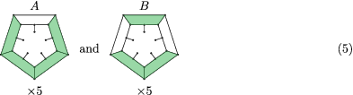
All other colorings of the cap yield either vertices that are not adjacent to a shaded face, or the unshaded faces are separated into two disconnected areas (by shading in all five faces that are adjacent to the boundary). It will be seen below that Hamilton cycles starting in cap-type A give rise to the term 5 × 2^k + 1, and type B to the term $5 \times 4 \times 1 2^{\frac{k}{2}} χ (k)$ .

Assume that the cap is shaded as A. One can easily show using Lemma 2 that only two layer types need to be considered for shading of all remaining layers (up to reflection). Using the notation introduced above, these are (1) and (1,2,3,4):

A (1,2,3,4)-layer must be followed by a (1)-layer in one of two ways, and a (1)-layer must be followed by a (1,2,3,4)-layer in one of two ways:

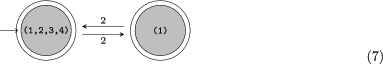
for which the adjacency matrix is:

A = (\begin{matrix} 0 & 2 \\ 2 & 0 \end{matrix}) .

()

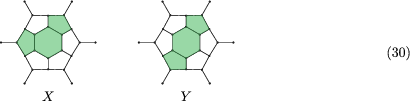
The possible end-cap shadings that can follow states (1) and (1,2,3,4) are W and X, respectively. W can follow state (1)in two ways and X can follow state (1,2,3,4) in two ways.

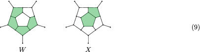
As state (1) can follow on cap A in one of two ways, and for each of (1) and (1,2,3,4), there is a cap which may follow in one of two ways, we obtain the two terminal adjacency matrices $(\begin{matrix} 2 & 0 \end{matrix})$ and $(\begin{matrix} 0 & 2 \\ 2 & 0 \end{matrix})$ . The number of Hamilton cycles of C_20 + 10k that originate from case A is:

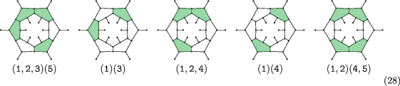
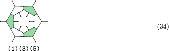
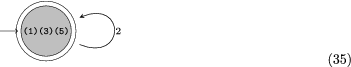
\begin{align} N_{HC}^{(A)} (k) & = 5 \times \sum ((\begin{matrix} 2 & 0 \end{matrix}) \times {(\begin{matrix} 0 & 2 \\ 2 & 0 \end{matrix})}^{k - 1} \times (\begin{matrix} 0 & 2 \\ 2 & 0 \end{matrix})) \end{align}

()

\begin{align} = 5 \times 2^{k + 1} . \end{align}

()

When case B is chosen for the cap, there are four layer types to be considered for shading in the remainder of the graph: (1,3), (1)(3), (1,2,4), and (1,2)(4).

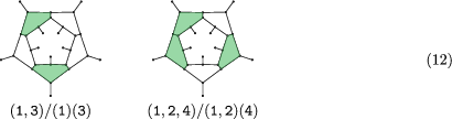
This is described by the following DFA, which with the order ((1,2)(4), (1,2,4), (1)(3), (1,3)) has the adjacency matrix B:

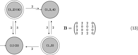
with accepting states corresponding to columns 1 and 4.

Cap B may be followed by (1,2,4) and (1)(3) in one of two ways each.

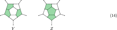
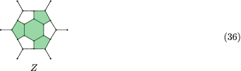
States (1,2)(4) and (1,3) may be followed by either of caps Y and Z in one of two ways each. No other caps are possible because shading the central last face differently would either yield multiple cycles by disconnecting the shaded or unshaded area, or exclude one vertex from the cycle, both violating Lemma 1.

Thus, the number of Hamilton cycles in C_20 + 10k that start from case B is

\begin{align} N_{HC}^{(B)} (k) & = 5 \times \sum ((\begin{matrix} 0 & 2 & 2 & 0 \end{matrix}) \times B^{k - 1} \times (\begin{matrix} 2 & 2 \\ 0 & 0 \\ 0 & 0 \\ 2 & 2 \end{matrix})) \end{align}

()

\begin{align} = 5 \times (B_{1, 2}^{k + 1} + B_{1, 3}^{k + 1}) . \end{align}

()

To understand the alternating term in Equation (4), we compute the first few powers of B:

B^{2} = (\begin{matrix} 6 & 0 & 0 & 6 \\ 0 & 6 & 6 & 0 \\ 0 & 6 & 6 & 0 \\ 6 & 0 & 0 & 6 \end{matrix}), B^{3} = (\begin{matrix} 0 & 24 & 24 & 0 \\ 18 & 0 & 0 & 18 \\ 18 & 0 & 0 & 18 \\ 0 & 24 & 24 & 0 \end{matrix}), B^{4} = (\begin{matrix} 72 & 0 & 0 & 72 \\ 0 & 72 & 72 & 0 \\ 0 & 72 & 72 & 0 \\ 72 & 0 & 0 & 72 \end{matrix}) .

()

We now prove the even and odd cases separately by induction. Assume for some odd k ≥ 1 that B^k + 1 is of the form $(\begin{matrix} x & 0 & 0 & x \\ 0 & x & x & 0 \\ 0 & x & x & 0 \\ x & 0 & 0 & x \end{matrix})$ . Then the next odd k yields:

B^{2} B^{k + 1} = (\begin{matrix} 6 & 0 & 0 & 6 \\ 0 & 6 & 6 & 0 \\ 0 & 6 & 6 & 0 \\ 6 & 0 & 0 & 6 \end{matrix}) (\begin{matrix} x & 0 & 0 & x \\ 0 & x & x & 0 \\ 0 & x & x & 0 \\ x & 0 & 0 & x \end{matrix}) = (\begin{matrix} 12 x & 0 & 0 & 12 x \\ 0 & 12 x & 12 x & 0 \\ 0 & 12 x & 12 x & 0 \\ 12 x & 0 & 0 & 12 x \end{matrix}) = 12 B^{k + 1} .

()

Since B² (the case k = 1) is of this form, we obtain by induction that B^k + 1 is of this form for every odd k ≥ 1, by which we obtain $B_{1, 2}^{k + 1} + B_{1, 3}^{k + 1} = 0$ for every odd k ≥ 1. That is, the number of Hamiltonian cycles starting in configuration B is 0 whenever the number of layers k is odd.

For the even case, assume for some even k ≥ 0 that B^k + 1 is of the form $(\begin{matrix} 0 & x & x & 0 \\ y & 0 & 0 & y \\ y & 0 & 0 & y \\ 0 & x & x & 0 \end{matrix})$ . Then the next even k gives:

B^{2} B^{k + 1} = (\begin{matrix} 6 & 0 & 0 & 6 \\ 0 & 6 & 6 & 0 \\ 0 & 6 & 6 & 0 \\ 6 & 0 & 0 & 6 \end{matrix}) (\begin{matrix} 0 & x & x & 0 \\ y & 0 & 0 & y \\ y & 0 & 0 & y \\ 0 & x & x & 0 \end{matrix}) = (\begin{matrix} 0 & 12 x & 12 x & 0 \\ 12 y & 0 & 0 & 12 y \\ 12 y & 0 & 0 & 12 y \\ 0 & 12 x & 12 x & 0 \end{matrix}) = 12 B^{k + 1} .

()

Since B (B^k + 1 for k = 0) is of this form, we obtain by induction that this holds for every even k ≥ 0. How many Hamilton cycles start in configuration B for k inner layers when k is even? For k = 0, we read off the number to be $5 \times (2 + 2) = 5 \times 4 \times 1 2^{\frac{0}{2}}$ . Finally, assuming the count is $5 \times 4 \times 1 2^{\frac{k - 2}{2}}$ for some even k − 2 ≥ 0, the count for k (by Equation 19) is

N_{HC}^{(B)} (k) = 5 \times 4 \times 1 2^{\frac{k - 2}{2}} \times 12 = 5 \times 4 \times 1 2^{\frac{k}{2}} (k even),

()

whereby, by induction, the formula holds for all even values of k ≥ 0. Together, Equations (10) and (20) complete the proof.

3.3 The number of Hamilton cycles in C_24 + 12k-D₆₊(6,0) nanotubes

We next turn to the number of Hamilton cycles in the C_24 + 12k-D₆₊(6,0) fullerene nanotube series, the next-thinnest class of layered nanotubes.

Theorem 3.The C_24 + 12k-D₆₊(6,0) fullerene nanotube $(k \in ℕ_{0})$ admits

N_{HC} (k) \approx 16 \times 2^{k} + 55.67911535839 \times 2^{2.1679870 k}

()

Hamilton cycles. The exact expression for the Hamilton cycle count is given in Equation (38).

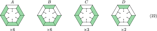
Proof.There are four inequivalent options for shading in the first cap of the graph up to D₆-symmetry, with multiplicities 6, 6, 3, and 2, respectively:

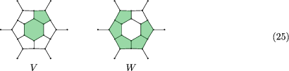
Starting from the first case (A) we need to consider only two different layer shadings (in analogy to case A of the previous proof), namely, (1,2,3,4,5) and (1):

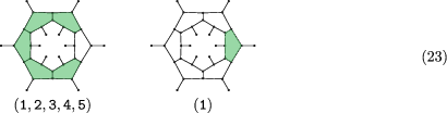
Both layers may follow each other according to the following graph:

which can be written as the adjacency matrix $U = (\begin{matrix} 0 & 2 \\ 2 & 0 \end{matrix})$ .

State (1,2,3,4,5) may follow on A in two ways, and states (1,2,3,4,5) and (1) may be followed by caps V and W respectively in two ways each.

The number of Hamilton cycles starting from cap A is therefore

\begin{align} N_{HC}^{(A)} (k) & = 6 \times \sum ((\begin{matrix} 2 & 0 \end{matrix}) \times {(\begin{matrix} 0 & 2 \\ 2 & 0 \end{matrix})}^{k - 1} \times (\begin{matrix} 0 & 2 \\ 2 & 0 \end{matrix})) \end{align}

()

\begin{align} = 6 \times (U_{1, 1}^{k + 1} + U_{1, 2}^{k + 1}) = 6 \times 2^{k + 1} . \end{align}

()

Caps B and C can be treated together because starting from either leads to the same options for shading in the remainder of the graph. We need to consider (1,2,3)(5), (1)(3), (1,2,4), (1)(4), and (1,2)(4,5).

We obtain the following graph V and adjacency matrix V:

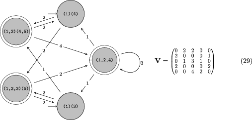
Cap B may be followed by (1)(3) and (1,2,4) in two ways each, while cap C may be followed by states (1,2,4) and (1)(4) in four and two ways, respectively.

There are two end caps. X may follow on states (1,2,3)(5) and (1,2,4) in two and one way, respectively, while Y may follow (1,2)(4,5) and (1,2,4) in two and one way, respectively.

Keeping in mind the multiplicities of the first layers, we get

\begin{align} N_{HC}^{(B)} (k) + N_{HC}^{(C)} (k) & = \sum ((\begin{matrix} 6 & 3 \end{matrix}) \times (\begin{matrix} 0 & 2 & 2 & 0 & 0 \\ 0 & 0 & 4 & 2 & 0 \end{matrix}) \times V^{k - 1} \times (\begin{matrix} 2 & 0 \\ 0 & 0 \\ 1 & 1 \\ 0 & 0 \\ 0 & 2 \end{matrix})) with \end{align}

()

\begin{align} N_{HC}^{(B)} (k) & = 6 \times (V_{1, 2}^{k + 1} + V_{1, 4}^{k + 1}) and \end{align}

()

\begin{align} N_{HC}^{(C)} (k) & = 3 \times (V_{5, 2}^{k + 1} + V_{5, 4}^{k + 1}) . \end{align}

()

Cap D only allows for choosing state (1)(3)(5) for all following layers.

However, there are two possible orientations for each layer.

There is one possible cap Z that may follow (1)(3)(5) in either of two ways.

The adjacency matrix is (2), yielding

N_{HC}^{(D)} (k) = 2 \times (2) \times {(2)}^{k - 1} \times (2) = 2 \times 2^{k + 1}

()

Hamilton cycles starting from cap D. In total the number N_HC of Hamilton cycles in C_24 + 12k (6,0) nanotubes is

\begin{align} N_{HC} (k) & = N_{HC}^{(A)} (k) + N_{HC}^{(B)} (k) + N_{HC}^{(C)} (k) + N_{HC}^{(D)} (k) \\ = 6 \times 2^{k + 1} + 6 \times (V_{1, 2}^{k + 1} + V_{1, 4}^{k + 1}) + 3 \times (V_{5, 2}^{k + 1} + V_{5, 4}^{k + 1}) + 2 \times 2^{k + 1} . \end{align}

()

Due to the complicated behavior of the matrix powers V^k, it is not possible to derive a simple closed form expression. However, while the exact counts have many complicated terms, they do asymptotically approach simple exponentials: $(V_{1, 2}^{k} + V_{1, 4}^{k}) \to 1.0862679 \times 2^{2.1679870 k}$ , and $(V_{5, 2}^{k} + V_{5, 4}^{k}) \to 1.9573872 \times 2^{2.1679870 k}$ , yielding 16-digit accuracy already at k = 35, improving as k grows (tested up to k = 3000). Hence, a simple approximate expression can be found:

\begin{align} N_{HC} (k) & = N_{HC}^{(A)} (k) + N_{HC}^{(B)} (k) + N_{HC}^{(C)} (k) + N_{HC}^{(D)} (k) \\ \approx 16 \times 2^{k} + 55.67911535839 \times 2^{2.1679870 k} . \end{align}

()

3.4 Long-range exponential behavior of C_20 + 10k-D₅₊ nanotube series versus C_24 + 12j-D₆₊ series

Our original interest in finding expressions for the Hamiltonian cycle counts of the infinite series was due to our work in Reference 11, which originally suggested that the C_20 + 10k-D₅₊ series defined both strict upper and lower bounds to the number of Hamiltonian cycles admitted by any fullerene graphs. This was verified for the tens of millions of graphs up to C₁₂₀. However, while the conjecture that this D_5d nanotube series maximizes Hamiltonian cycle count looked extremely plausible, the exact expressions allowed us to produce a counter-example—in a region that could never have been checked exhaustively by existing methods.

The crossover-point is C₁₀₂₀ = C_{24 + 83 × 12} = C_{20 + 100 × 10} (i.e., k = 100 and j = 83). From C₁₀₂₀ on, every C_24 + 12j-D₆₊ break the conjectured upper bound due to the larger exponent taking over. C₁₀₂₀-D_5d has

N_{HC} (C_{1020} - D_{5 d}) =_{18, 200, 876, 300, 004, 299, 546, 655, 183, 227, 191, 134, 932, 148, 320, 173, 545, 226, 240}

()

Hamiltonian cycles (i.e., 1.820 × 10⁵⁵) but C₁₀₈₀-D_6d has

N_{HC} (C_{1020} - D_{6 d}) =_{18, 250, 747, 738, 371, 979, 597, 388, 745, 176, 681, 058, 911, 549, 835, 175, 654, 326, 272}

()

(i.e., 1.825 × 10⁵⁵). After that, the D₆₊ series takes over forever (but may be overtaken by other series), as seen in Figure 8.

4 Proof of Theorem 1

Proof.(i) Consider a Hamilton cycle admitted by G_k = A ⊕ L₁ ⊕ ⋯ ⊕ L_k ⊕ Z represented through Lemma 1 as a face shading S. We can decompose S into shadings of the subgraph components, $S = S_{A} \oplus S_{L_{1}} \oplus \dots \oplus S_{L_{k}} \oplus S_{Z}$ .

Each shaded subgraph corresponds to a unique node in the DFA connected through a path from start to end. We prove the property by induction. For notational convenience, write S₀ = S_A, S_k + 1 = S_Z, and $S_{i} = S_{L_{i}}$ for i = 1, ⋯ , k.

Since by Lemma 1, S fulfills property (a)–(c), so must also S_A, S_Z, and S₁, ⋯ , S_k (where, for property (c), we consider two faces connected in a sub-component if they are either connected within that component, or determined to be so from the connectedness-label). In particular, S_A = S₀ and S_Z = S_k + 1 are nodes in the DFA by Step I.1.

We show that the appropriately connectedness-labeled shadings S₁, ⋯ , S_k are nodes in the automaton, and S₀ → S₁ → ⋯ → S_k + 1 is a path over it. This is done by induction over the length i of the sub-path S₀ → ⋯ → S_i.

i = 0: The node for S₁ is created in I.1 if k = 0, or R.1 in the first iteration if S₁ is an internal layer. In both cases, the arc S₀ → S₁ is created in the first iteration of Step R.1.

i ⇒ i + 1: Assume now for 1 ≤ i ≤ k that the path S₀ → S₁ → ⋯ → S_i exists. Then, at some step j ≤ i, the connectedness-labeled shading S_i is extracted in Step R.1, and since S_i ⊕ S_i + 1 must fulfill L1 (a)–(c) (or S would not be a Hamilton cycle), the appropriately connectedness-labeled S_i + 1 is added together with the arc S_i → S_i + 1 at latest in Step R.3 of iteration j ≤ i.

The caps are not connectedness-labeled, but are not needed to be, as this information is only needed to maintain Lemma 1(c) through Lemma 2 in the induction step.

(ii) We show that every path beginning in an initial state and ends in a final state corresponds to a Hamilton cycle, and the product of the arc labels along the path is the number of Hamilton cycles that correspond to this path through (i).

Consider such a path S₀ → ⋯ → S_k + 1. By construction, a node for the connectedness-labeled shading S_i is created if either S_i is a cap-shading, or if S_i − 1 ⊕ S_i fulfills property (a) and (b), and does prevent (c) in the future. By Lemma 2, this then extends to all of S₀ ⊕ S₁ ⊕ ⋯ ⊕ S_i. The final arc to the end-cap S_k → S_k + 1 is placed if and only if it closes correctly, so that S = S₀ ⊕ S₁ ⊕ ⋯ ⊕ S_k ⊕ S_k + 1 fulfills all of (a), (b), and (c). Thus, S represents a Hamilton cycle by Lemma 2.

Since at each step, the arc is labeled with the number of equivalent ways to orient the shading S_i + 1, the product yields the total number of Hamilton cycles that are represented by this path.

(iii) By the above, every Hamilton cycle maps uniquely to a path $S_{0} \to_{}^{m_{01}} S_{1} \to_{}^{m_{12}} \dots \to_{}^{m_{k, k + 1}} S_{k + 1}$ starting in an initial state S₀ and ending in a final state S₂, such that the product m₀₁m₁₂ ⋯ m_{k, k + 1} is the number of Hamilton cycles that map to this same path. The total number of Hamilton cycles admitted by G_k is then the sum of these products over all such paths of length k. Letting M be the adjacency matrix of the state machine M with m_st nonzero whenever $s \to_{}^{m_{s t}} t$ is an arc in M, this is exactly calculated by

N_{HC} (G_{k}) = \sum_{\begin{matrix} s \in Initial \\ t \in Final \end{matrix}} M_{s t}^{k} .

()

ACKNOWLEDGEMENTS

L. N. W. thanks Alexander von Humboldt Foundation for a Feodor Lynen fellowship. P. S. is indebted to the Alexander von Humboldt Foundation (Bonn) for financial support. J. A. was was funded by the VILLUM Foundation (Villum Experiment Project 00023321, “Folding Carbon: A Calculus of Molecular Origami”).

CONFLICT OF INTEREST

This work does not have any conflicts of interest.

Biographies

Lukas N. Wirz received his Diploma degree in Chemistry from Heidelberg University, followed by a Ph.D. in theoretical chemistry at Massey University. As postdoc at Hylleraas Centre for Quantum Molecular Sciences, U. of Oslo, and Feodor-Lynen fellow at University of Helsinki Dep. of Chemistry, he worked on quantum chemical method development. He is now a 3D imaging specialist at Planmeca.
Peter Schwerdtfeger holds a chair in Theoretical Chemistry at Massey University and is currently Head of the Institute for Advanced Study. He holds degrees in chemical engineering, chemistry and mathematics and received habilitation at Marburg University. He earned many awards, amongst them Fellowships of the Royal Society New Zealand and the International Academy of Quantum Molecular Science, the Humboldt Research Prize, Fukui Medal, Rutherford medal, and most recently the Dan Walls medal in physics. His research interests are in fundamental chemistry and physics.
James Avery is associate professor of Computations in Physics at the Niels Bohr Institute, University of Copenhagen. He holds degrees in computer science and mathematics, but works where computer science and math meet theoretical chemistry and physics. His current grant, Folding Carbon: a Calculus for Molecular Origami explores how combinatorial geometry determines molecular shapes and electronic structure of polyhedral molecules.

References

1Karp RM. Reducibility among combinatorial problems. In: RE Miller, JW Thatcher, eds. Complexity of Computer Computations. Berlin, Germany: Plenum Press; 1972: 85-103.
10.1007/978-1-4684-2001-2_9
Google Scholar
2Rubin F. A search procedure for Hamilton paths and circuits. J ACM. 1974; 21(4): 576-580. https://doi.org/10.1145/321850.321854.
10.1145/321850.321854
Web of Science® Google Scholar
3Garey MR, Johnson DS. Computers and Intractability: A Guide to the Theory of NP-Completeness. New York, NY: Oxford University Press; 1983.
Google Scholar
4Valiant LG. The complexity of enumeration and reliability problems. SIAM J Comput. 1979; 8(3): 410-421. https://doi.org/10.1137/0208032.
10.1137/0208032
Web of Science® Google Scholar
5Liśkiewicz M, Ogihara M, Toda S. The complexity of counting self-avoiding walks in subgraphs of two-dimensional grids and hypercubes. Theor Comput Sci. 2003; 304(1): 129-156. https://doi.org/10.1016/S0304-3975(03)00080-X.
10.1016/S0304-3975(03)00080-X
Web of Science® Google Scholar
6Wilson RJ. A brief history of Hamiltonian graphs. In: LD Andersen, IT Jakobsen, C Thomassen, B Toft, PD Vestergaard, eds. Graph Theory in Memory of G.A. Dirac, Vol. 41 of Annals of Discrete Mathematics. Elsevier: Amsterdam; 1988: 487-496. https://doi.org/10.1016/S0167-5060(08)70484-9.
10.1016/S0167-5060(08)70484-9
Google Scholar
7Wirz LN, Schwerdtfeger P, Avery JE. Naming polyhedra by general face-spirals – theory and applications to fullerenes and other polyhedral molecules. Fuller Nanotub Carbon Nanostruct. 2018; 26(10): 607-630. https://doi.org/10.1080/1536383X.2017.1388231.
10.1080/1536383X.2017.1388231
CAS Web of Science® Google Scholar
8Schwerdtfeger P, Wirz L, Avery J. Program fullerene: a software package for constructing and analyzing structures of regular fullerenes. J Comput Chem. 2013; 34(17): 1508-1526. https://doi.org/10.1002/jcc.23278.
10.1002/jcc.23278
CAS PubMed Web of Science® Google Scholar
9Franzblau DS. Construction of Hamiltonian cycles in layered cubic planar graphs. Graphs Comb. 2002; 18(2): 259-270. https://doi.org/10.1007/s003730200019.
10.1007/s003730200019
Web of Science® Google Scholar
10Kutnar K, Marušiš D. On cyclic edge-connectivity of fullerenes. Discr Appl Math. 2008; 156(10): 1661-1669. https://doi.org/10.1016/j.dam.2007.08.046.
10.1016/j.dam.2007.08.046
Web of Science® Google Scholar
11Avery J, Wirz LN, Babić D, Schwerdtfeger P. Exponentially many Hamilton cycles in fullerenes: explicit probabilistic upper and lower bounds (in preparation).
Google Scholar

Citing Literature

All articles

Calculating the number of Hamilton cycles in layered polyhedral graphs

Abstract

1 Introduction

2 Counting Hamilton cycles in a cubic polyhedral graph

2.1 An acyclic finite state-machine that counts Hamilton cycles in polyhedral graphs

2.2 A cyclic finite state-machine that counts Hamilton cycles in infinite series of polyhedral graphs

3 Examples

3.1 Syntax

3.2 The number of Hamilton cycles in C_20 + 10k-D₅₊(5,0) nanotubes

3.3 The number of Hamilton cycles in C_24 + 12k-D₆₊(6,0) nanotubes

3.4 Long-range exponential behavior of C_20 + 10k-D₅₊ nanotube series versus C_24 + 12j-D₆₊ series

4 Proof of Theorem 1

ACKNOWLEDGEMENTS

CONFLICT OF INTEREST

Biographies

References

Citing Literature

Figures

References

Information

About Wiley Online Library

Help & Support

Opportunities

Connect with Wiley

Calculating the number of Hamilton cycles in layered polyhedral graphs

Abstract

1 Introduction

2 Counting Hamilton cycles in a cubic polyhedral graph

2.1 An acyclic finite state-machine that counts Hamilton cycles in polyhedral graphs

2.2 A cyclic finite state-machine that counts Hamilton cycles in infinite series of polyhedral graphs

3 Examples

3.1 Syntax

3.2 The number of Hamilton cycles in C20 + 10k-D5+(5,0) nanotubes

3.3 The number of Hamilton cycles in C24 + 12k-D6+(6,0) nanotubes

3.4 Long-range exponential behavior of C20 + 10k-D5+ nanotube series versus C24 + 12j-D6+ series

4 Proof of Theorem 1

ACKNOWLEDGEMENTS

CONFLICT OF INTEREST

Biographies

References

Citing Literature

Figures

References

Related

Information

3.2 The number of Hamilton cycles in C_20 + 10k-D₅₊(5,0) nanotubes

3.3 The number of Hamilton cycles in C_24 + 12k-D₆₊(6,0) nanotubes

3.4 Long-range exponential behavior of C_20 + 10k-D₅₊ nanotube series versus C_24 + 12j-D₆₊ series