Robust tracking design for uncertain MIMO systems using proportional–integral controller of order v
Abstract
This paper provides a systematic method to design robust tracking controllers of reference signals with bounded derivatives of order ν for uncertain multi-input multi-output (MIMO) systems with bounded parametric uncertainties, in particular, of rational multi-affine type, and/or in presence of disturbances with bounded derivatives of order ν. The proposed controllers have state-feedback structures combined with proportional–integral regulators of order ν (PIν). Theoretical tools and systematic methodologies are provided to effectively design robust controllers for the considered systems, also in case of additional bounded nonlinearities and/or not directly measurable states. Applicability and efficiency of the proposed methods are validated through three examples: the first one is theoretical and useful to validate the proposed methodology, the second case study presents a metal-cutting problem for an industrial robot, and the third example deals with a composite robot, such as a milling machine.
1 INTRODUCTION
Numerous industrial systems operate subject to parametric uncertainties and non-standard references and disturbances, which need to be efficiently controlled. For such systems evolving in an increasingly dynamic and global society, it is indispensable to design robust controllers able to track rapidly varying reference signals (i.e., with larger derivatives) quickly and precisely, despite any external disturbances. A number of publications on this topic are available (e.g. [1-7]), including recent ones [8-20]. However, the following practical limitations still remain in effect: (a) the considered classes of systems are often of particular structure; (b) the considered reference signals and disturbances almost always have standard waveforms (polynomial and/or sinusoidal ones); (c) the controllers are not robust enough and/or do not applicable to systems satisfying more than one specification; (d) the control inputs are excessive and/or unfeasible in some cases [1-11, 21-28].
A basic control problem is to force an uncertain process or a plant to track with an acceptable precision sufficiently smooth but generic references, e.g., with bounded ν - order derivatives and/or in the presence of generic but sufficiently smooth disturbances. This paper provides a systematic method to design robust tracking controllers using the majorant systems approach for LTI uncertain multi-input multi-output (MIMO) systems with bounded parametric uncertainties, in particular, of rational multi-affine type, and reference signals and disturbances with bounded derivatives of order ν. The proposed controller possesses a state-feedback structure combined with a PIν regulator. Systems with additional bounded nonlinearities and/or not directly measurable states are also considered.
This development presents a broad generalization of [29], where the case v = 1 has been considered with more restrictive uncertainty type and a controller without proportional action. The obtained results also generalize the results of [30] concerning uncertain MIMO systems, considering bounded uncertainties of rational multi-affine type, with an integral controller and observer. The applied majorant systems approach has already successfully used for particular classes of linear and nonlinear systems (see [29-31]). Another approach to design robust tracking controllers for relevant classes of nonlinear systems can be found in [32]. The provided results are particularly useful for mechatronic systems (e.g., rigid Cartesian robots, rolling mills, AGVs, conveyor belts, active suspension systems, printing machines), whose reference signals and disturbances are represented by non-standard waveforms (see, e.g., [30, 33, 34]).
Some distinctive features and advantages of the proposed study are: (a) The designed controllers avoid the derivative action causing realization problems, especially in the presence of measurement noises; (b) the presence of realistic uncertainties, which are bounded and, in particular, of rational multi-affine type; (c) the possibility to obtain acceptable tracking errors for reference signals and disturbances represented by generic sufficiently regular non-standard waveforms.
The paper is organized as follows. In Section 2, the considered MIMO uncertain systems are introduced, and the synthesis problems are stated. Section 3 provides the theoretical background. Section 4 presents the main theorems used to design robust controllers for the considered systems. Section 5 extends some results obtained in Section 4. Section 6 specifies the control design algorithms based on the presented theoretical background. In Section 7, three examples are provided: the first one is given to illustrate the proposed methodology, the second example presents a metal-cutting problem for an industrial robot, and the third case study considers a composite robot such as a milling machine, to show practical advantages and effectiveness of the designed controller. Finally, Section 8 presents conclusions and future developments to this study.
2 PRELIMINARIES AND PROBLEM STATEMENT
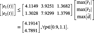
 (1)
(1) is a compact set.
Given a p.d. matrix P ∈ Rn×n, λmax(P) (λmin(P)) denotes the maximum (minimum) eigenvalue of P.
Given a real matrix A ∈ Rn×n, λ(A) is the set of eigenvalues (spectrum) of
 is the maximum real part of the eigenvalues of A, i.e.,
 denotes the maximum time constant of A;
 is an upper estimate of
 ;
;
 is an upper estimate of
 .
.
Let Α = {aij} be a real n × m matrix. |Α| is its absolute values matrix, i.e., |Α| = {|aij|}..
Given a function f (t), f (v)(t) denotes its derivative of v - th order.
 (2)
(2) , the conditions
 (3)
(3)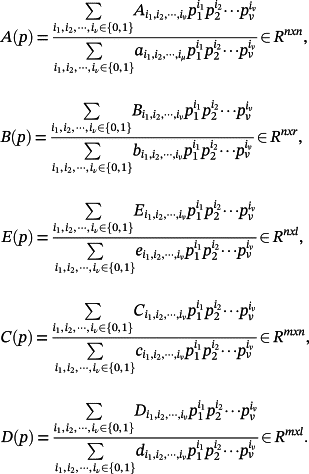 (4)
(4)In the following, for simplicity of notation, the explicit dependency of A(p), B(p), E(p), C(p), D(p) on p will be omitted.
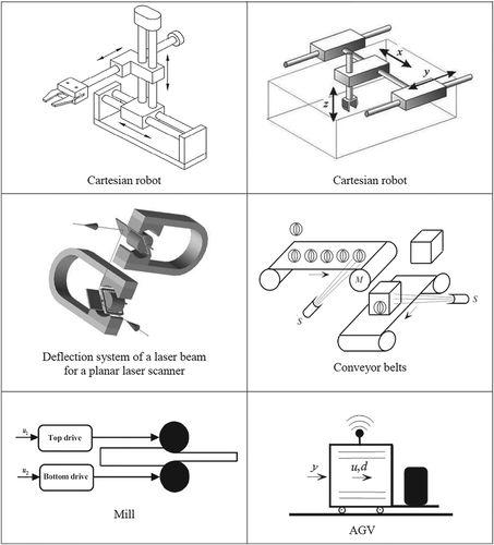
Remark 1.The considered class of systems is relevant from the engineering point of view, since many mechatronic and transportation processes are described by models referable to them (see Figure 1).
Remark 2.Note that many mechanical, electrical, mechatronic, thermal, and fluid dynamic systems can be modeled by systems in the form
 where matrices L,M,N are linear with respect to the physical system parameters, which are often uncertain. Hence, the dependency on uncertain parameters of the matrices A and B is of rational multi-affine type (or transformable to this by using suitable changes of the parameters, as demonstrated in Corollaries 1 and 2).
Remark 3.Conditions 3 imply that rank C = m ≤ n and rank B ≥ m, i.e., the m outputs of the plant are independent and the number of the independent control inputs has to be greater or at least equal to the number of the outputs to be controlled.
Suppose that the system 2 is controlled using a PIν controller with a state-feedback structure as shown in Figure 2.

 (5)
(5) (6)
(6)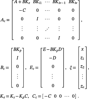 (7)
(7) of the closed-loop control system and the maximum norm
 of the tracking error e(t) of a generic reference signal r with an almost everywhere bounded derivative of order v, in the presence of a generic disturbance d with an almost everywhere bounded derivative of v - th order, and use
 and
and
 as parameters for the subsequent controller design. In other words, the objective is to find:
- a constant τc > 0 such that
 where Ac(p) is the dynamics matrix of the closed-loop control system,
 - non-negative constants Hr and Hd, called “generalized gain constants”, such that, after a possible transient phase, the tracking error satisfies the conditions
 (8)
(8)
Remark 4.Nowadays, a generic reference signal for a manufacturing or transportation system is a non-standard (non-polynomial or non-sinusoidal) signal, whose derivative represents “working velocity” or “transportation velocity”, while the second derivative represents acceleration.
In regard to the above systems, it can also be useful to compute the maximum norms
 of the tracking errors
 of
of
 since high values of
 can produce high-frequency oscillations and/or vibrations, while high values of
 can produce skids (e.g., for some transportation systems), and/or require high values of the control action.
Remark 5.A reference signal r(t) with a bounded v - th derivative can be obtained by interpolating a set of given points (tk, rk), k = 0, 1, …, nr, with appropriate splines or by filtering any piecewise constant or piecewise linear signal
 with the following MIMO filter:
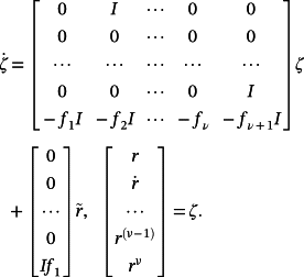 (9)
(9)In this case, it is also possible to reduce the control action, in particular, during the transient phase by suitably choosing initial conditions of the filter and its cutoff frequency.
Note that if the filter is a Bessel one with cutoff angular frequency ωb, larger or equal to the angular frequency of
 , then
 .
.
To solve the stated problem, the following preliminaries are given.
3 THEORETICAL BACKGROUND
Definition 1.Given the system
 (10)
(10) (11)
(11) and p ∈ ℘ , is said to be a majorant system of the system 10.
 (12)
(12) and
and
 .
. (13)
(13) (14)
(14)The following lemmas and corollaries hold (see [29, 30] for proofs).
Lemma 1.Consider a matrix H(p) (12) and a symmetric p.d. matrix P ∈ Rn×n. Then, i l = n,
 , where Q(p) = HT(p)P+PH(p), is achieved in one of the 2μ vertices Vp of ℘. Similarly,
 .
.
Corollary 1.Let
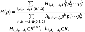 (15)
(15) where Q(p) = HT(p)P+PH(p), is given by
 where Vap is the set of 22μ vertices of
 ,
,
 and Ha(pa) is obtained from matrix H(p) by replacing
 with the product pipμ+i i = 1,2,…,μ. Similarly, an upper estimate of
 is given by
 .
.
Corollary 2.Let
 (16)
(16) Q(g(π)) = HT(g(π))P+PH(g(π)), is given by
 where Vp is the set of vertices of
 (17)
(17)Similarly, an upper estimate of
 is given by
 .
.
Lemma 2.Let A ∈ Rn×n be a matrix with ν real distinct eigenvalues λi,i = 1,…,ν, and
 distinct pairs of complex conjugate eigenvalues λh± = αh ± jωh, h = 1,…,μ, and let ui,i = 1,…,ν, and uh± = uah ± jubh,h = 1,…,μ, be the associated eigenvectors. Then, denoting as Z* the conjugate transpose of the matrix of the eigenvectors Z = [u1… uν ua1+jub1 ua1 − jub1… uaμ+jubμuaμ − jubμ], the matrix
 (18)
(18) (19)
(19)
Taking Remark 2 into account, it is important to analyze uncertain LTI MIMO systems, whose matrices are ratios of multi-affine functions with respect to the uncertain parameters. Concerning this, the following lemmas (see [29, 30] for proofs) are useful.
Lemma 3.Given the system
 (20)
(20) (21)
(21) (22)
(22)Lemma 4.Given the system
 (23)
(23) (24)
(24)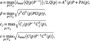 (25)
(25)Remark 6.Note that the majorant 21 yields an upper estimate for evolution of the system 20 for each t ∈ R, x0 ∈ Rn, p ∈ [p−, p+], u(t) : ‖u(t)‖ ≤ U, w(t) : ‖w(t)‖ ≤ W.
 (26)
(26)Similarly, the majorants 24 yield an upper estimate for evolution of the absolute value of each output yi (or ‖y(t)‖) of system 23 for each

Evidently, it depends on P how close this estimate would be to the real value. An inappropriate choice of P may result in a positive value of α, even if A(p) has all eigenvalues with negative real parts ∀p ∈ ℘.
If for an assigned
 the matrix
 has distinct eigenvalues (which is an easily verifiable condition), the corresponding matrix
 given by 18 is always p.d., and the equality 19,
 , always holds, even if
 has some eigenvalues with non-negative real parts.
A better estimate of the maximum absolute output values of the system 23, but more difficult to compute, can be obtained using the following theorem. This estimate is also valid in case of uncertain matrices of non-multi-affine type and in the presence of an additional bounded nonlinearity γ.
Theorem 1.Given the system
 (27)
(27) υ ∈ Rv is an external signal, and A, B, C are constant matrices of appropriate dimensions. Then,
 (28)
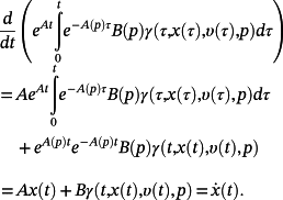
(28)Proof.Note that the solution to the system 27 satisfies the equation
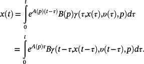 (29)
(29)Indeed,
 (30)
(30)The equation 29 implies that
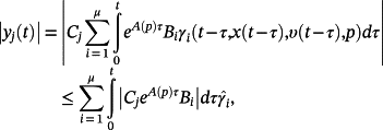 (31)
(31) are the j-th rows of γ,
 , respectively. The inequality 28 follows from 31 and the second last introduced notation, i.e., |{ fij}| = {|fij|}.
4 CONTROLLER DESIGN
This section presents the main results allowing one to design robust controllers to track generic reference signals with an acceptable precision, despite the presence of disturbances with bounded ν-th order derivatives.
 (32)
(32)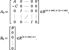 (33)
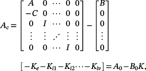
(33)Hence, if (A0, B0) is reachable, it is well-known that the eigenvalues of Ac can be assigned arbitrarily for a pre-fixed p by making a suitable choice of K, taking into account that they are placed symmetrically with respect to the real axis of the complex plane.
Concerning reachability of the pair (A0, B0), the following result holds.
Theorem 2.Let A ∈ Rn×n,B ∈ Rn×r,C ∈ Rm×n be a triple of matrices. If
 (34)
(34)Proof.Given a pair of matrices (F ∈ Rv × v,G ∈ Rv × ρ). If
 (35)
(35) (36)
(36)(A0, B0) is reachable.
Since (by swapping some columns)
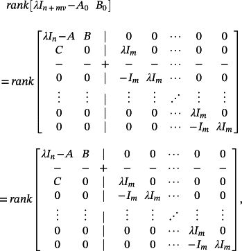 (37)
(37)The following theorems are useful to compute majorants of the control system.
Theorem 3.The control system 6 can also be represented as
 (38)
(38)Proof.Upon making the change of variables
 (39)
(39) (40)
(40)From 6, it follows that
 (41)
(41)Now, the first equation of 38 follows from 39, 40, and 41.
The first equation in 6 and 39 implies that
 (42)
(42)Corollary 4.Consider the control system (6). If r(t) and d(t) have bounded derivatives of order v+μ, μ ≥ 1, and are equal to zero for t = 0, then
 (46)
(46)Proof.Denoting as F(s) = L(f(t)) the Laplace transform of a generic function f(t), one obtains E(s) = H(sI − Ac)−1sν(BcR(s)+EcD(s)).
Hence, L(e(μ)(t)) = sμE(s) = H(sI − Ac)−1sν+μ(BcR(s)+EcD(s)), and the proof follows.
The control system 38 is observable, considering the tracking error e(t) as the output, since the following theorem states.
Theorem 4.If the pair of matrices (A ∈ Rn × n, C ∈ Rm × n) is observable, then the pair of matrices (Ac, H) is also observable.
Proof.The proof readily follows by noting that
 (47)
(47)Consider now the control system in Figure 2, where the plant is given by 2. In view of Theorem 3, this control system can be represented as
 (48)
(48)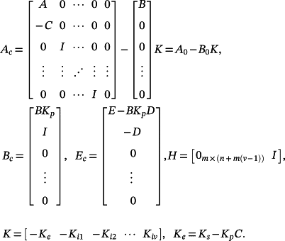 (49)
(49)The following main theorem holds.
Theorem 5.Suppose that the plant 2 satisfies the condition 3 and ℘ = [p−, p+]. If
 is the nominal value of p then there exists a matrix K such that the eigenvalues of the matrix
 are equal to n+vm pre-fixed symmetric values
 of ℂ. In addition, if the eigenvalues
 are distinct, then, ∀r(t), d(t) : ‖r(v)(t)‖ ≤ Rν,‖d(v)(t)‖ ≤ Dν, a majorant of the system 48 is given by
 (50)
(50) (51)
(51) (52)
(52)
 ,
,
 is the matrix of the eigenvectors of
 and Vp being the set of vertices of the hyper-rectangle ℘.
Remark 7.Note that if
 and all the eigenvalues of Ac have negative real parts, the time constant τc = − 1/ac of the majorant system is positive and coincides, in view of Lemma 2, with the maximum time constant
 of the control system.
 (53)
(53) (54)
(54)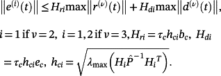 (55)
(55)Similar estimates of
 , j = 1,...,m, i = 0,1,2, can be obtained using Lemma 4, Theorems 1, 3, and Corollaries 3, 4.
Remark 8.Given a reference signal r(t), the change of variable t = τ/ρ yields
 ,
,
 Hence, halving “velocity” (i.e., assuming ρ = 2) makes the second derivative (“acceleration”) four times less and reduces the maximum tracking error accordingly. Dividing the “velocity” by three (ρ = 3) makes the second derivative (“acceleration”) nine times less, etc. Similarly, if “velocity” is halved (ρ = 2), the third derivative becomes eight times less, and the maximum tracking error is reduced accordingly.
Remark 9.It is well-known that the proportional action makes the control system faster and generally leads to a reduction of the error e(t). On the other hand, the control signal may increase due to sudden variations of r(t) and/or d(t). For example, if ζ0 = 0, then u(0) = Kp(r(0) − Dd(0)). Hence, it is appropriate to make the matrix Kp bounded,
 Note that once the matrix K (and, therefore, the matrix Ke) is computed, for a fixed matrix Kp the relation Ke = Ks − KpC implies Ks = KpC+Ke.
If the initial state of the control system is not very large (which can be obtained using a suitably filtered reference or using an appropriate joint reference signal before the desired reference), the matrix Kp can be chosen such that for
 the tracking error norm ‖e‖ depends on ‖r(v+1)(t)‖ and not on ‖r(v)(t)‖. Indeed, the following theorem holds.
Theorem 6.For
 it is possible to choose a matrix Kp such that
 (56)
(56)Proof.For prefixed eigenvalues of
 and, hence, of K, one obtains
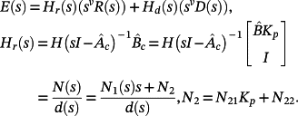 (57)
(57)Therefore, it is possible to choose Kp such that N2 = 0 and then, from the relation
 to compute Ks and Ki. Making such a choice of Kp it is E(s) = Hr(s)(svR(s)) = (N1(s)/d(s))(sν+1R(s)), from which 56 follows.
5 EXTENSIONS
The methodology provided in the previous sections can be used to establish other new results. In the following, for brevity, only two are stated in the case v = 1. The first result deals with the case of systems with unmeasurable states, and the second one treats a class of nonlinear system with additional bounded nonlinearities.
5.1 Observer-based controller
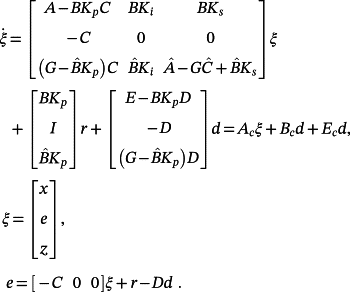
 (58)
(58)
 is the nominal value of p and G is a design matrix.
 (59)
(59)
 (62)
(62)Therefore, if
 , the separation principle for eigenvalues is valid. Specifically, note that if d ≠ 0 and/or
 , the observer does not provide the state of the system and, hence, has to be considered as a dynamic compensator.
 (63)
(63) .
.5.2 Systems with additional bounded nonlinearities
 (64)
(64)Since the nonlinearity g is bounded, if
 is also bounded, the controller can be designed via the majorant system approach using Lemmas 3, 4 or via input–output (i-o) increase, applying Theorem 1 to the control system 68.
Remark 10.Clearly, the tracking error can be acceptable using the proposed controller also if the nonlinearity g is not bounded, but bounded in a sufficiently large neighborhood,
 and the initial state of the control system are sufficiently bounded.
An estimate of the asymptotic practical stability region can be determined via majorant system (see 33 in [30]) or via randomized simulations [35].
6 DESIGN ALGORITHMS
In this section, some algorithmic procedures to design robust controllers are provided.
Remark 11.Once K and Kp are fixed, some less conservative (smaller) values of τc, Hr and Hd can be obtained using the following algorithm.
Algorithm.
- Step 1
Divide the set ℘ in N hyper-rectangles
 .
. - Step 2
Determine the majorant systems corresponding to each hyper-rectangle ℘i, with
 or equal to a close value, if cond(Pi) ≫ 1. Then, compute the corresponding values of aci,Hr i and Hd i by (51)-(53).
 - Step 3
Compute αc,τc,Hr and Hd by using the relations
 (69)
(69)Similar algorithms can be developed, if the majorants of the control systems are computed using Lemma 4 and Theorem 1 for each
 .
.
Remark 12.A majorant system of the i-o type can be obtained as an envelope of N majorant systems.
Remark 13.Since the pair (A0, B0) is reachable in view of Theorem 2, the eigenvalues of Ac can be assigned arbitrarily for a fixed p. Furthermore, in view of Theorem 4, the control system is observable, considering the tracking error e(t) as output. Hence, suitably choosing the matrices K and Kp, it is possible to stabilize the control system and optimize a quality index related to the tracking error.
Let
 be the nominal value of p. The eigenvalues of
 can be chosen equal to g Λ, where g is a positive real optimization parameter belonging to an interval or set ϒ, and Λ is a set of n+mv complex numbers with negative real parts, symmetric with respect to the real axis. A good choice of Λ is to consider the set of poles ΛB of a low-pass n+mv-th order Butterworth (Bessel) filter with cutoff frequency ωn = 1, or the set of poles with real parts equal to −1 and imaginary parts such that the pole arguments are equal to the ones of ΛB, or a set of n+mv poles belonging to the trapezoidal region
 .
.
- For instance, for a desired maximum error
 , setting e = HrRν+HdDν, the design algorithm consists in solving the min-max conditioned problem
 (70)
(70)This problem can be solved by using the Matlab commands place and fmincon (see e.g. [27]).
 then 70 provides the controller minimizing e. If the obtained tracking error is not satisfactory, then it is possible to reduce the velocity of r(t) by a factor ρ (see Remark 8).
- It is also possible to design a controller solving the min-max conditioned problem
 (71)
(71) is the desired maximum time constant. Then, compute Hr and Hd to obtain an estimate of the maximum value of e.
- Finally, it is possible to design a controller minimizing the performance index
 (72)
(72)7 EXAMPLES
Three examples are provided: the first one is theoretical to illustrate the proposed methodology; the second and third ones are industrial, whose objective is to demonstrate utility and feasibility of the stated results and effectiveness of the designed controller.
Example 1.Consider the plant
 (73)
(73)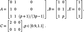 (74)
(74)The objective is to design controllers to force the plant 73 to track sufficiently smooth reference signals with acceptable errors. In the following, the cases ν = 1 and ν = 2 are considered.
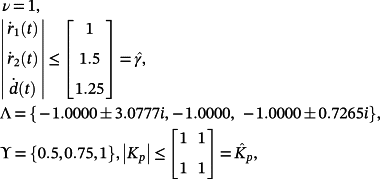 (75)
(75) (76)
(76) (77)
(77)For the reference signals and disturbance shown in Figure 4, the tracking errors obtained for p ∈ [0.9,1.1] with increments by 0.025 are displayed in Figure 5.
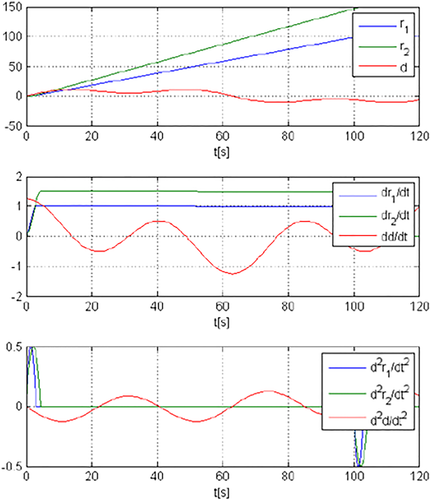

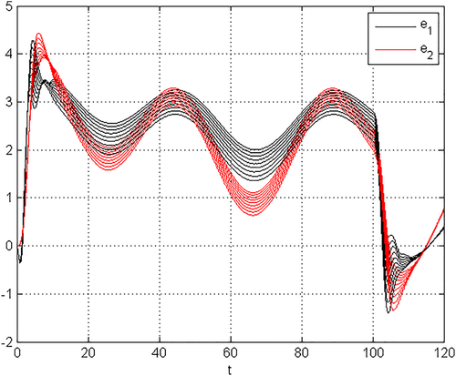
Figure 5 shows that ‖e(t)‖ ≤ 5.9125, whereas using the provided Algorithm with Lemma 4 and N = 20 yields ‖e(t)‖ ≤ 8.4116.
 is numerically calculated as
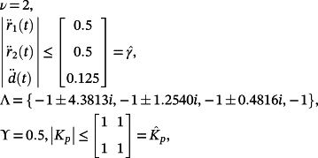
 whereas the estimate obtained by using the provided Algorithm with Lemma 4 and N = 20 is equal to τc = 2.8975. In addition, Theorem 1 implies that
 (78)
(78) (79)
(79) (80)
(80)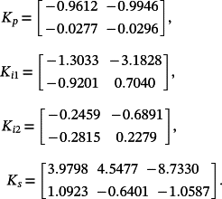 (81)
(81)For the reference signals and disturbance shown in Figure 4, the tracking errors obtained for p ∈ [0.9,1.1] with increments by 0.025 are displayed in Figure 6.
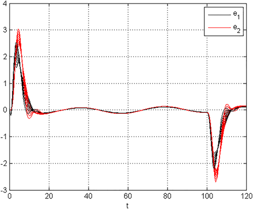
The maximum time constant
 is numerically calculated as
 whereas the estimate obtained by using the provided Algorithm with Lemma 4 and N = 20 is equal to τc = 3.5917.
Note that during the phase where
 the tracking error is smaller. Obviously, if also
 then after a transient phase the tracking error is null.
Example 2.Consider a Cartesian planar robot. Assuming that each activation system is an electric DC motor, the model of each axis is of the form 2 with
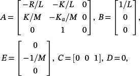 (83)
(83) ; i is measured in A, υ in cm/s, and y in cm.
Suppose that R = 1, L = 0.010, K = 5, M = 0.50, Ka = p ∈ [0.40,0.60].
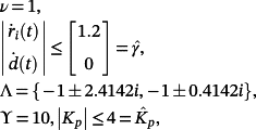 (84)
(84) (85)
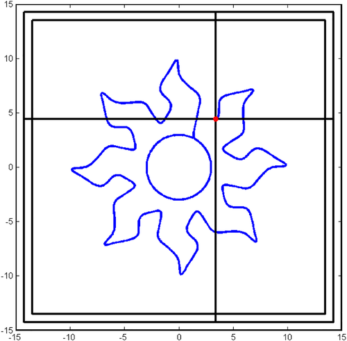
(85)Suppose that the robot's task is to cut the metal ring in Figure 7 from a metal sheet by using a laser beam with a constant cutting velocity in 120s.
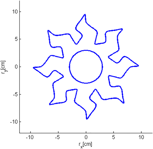
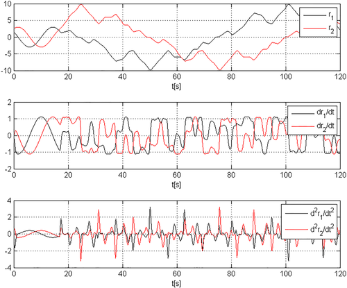
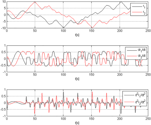
Figure 8 displays the smoothed reference signals r1 = rx and r2 = ry reported with the corresponding velocities and accelerations, which are obtained by using two third-order single-input single-output (SISO) Bessel filters with ωb = 5rad/s (initial conditions [ri(0) 0 0]T, i = 1,2) from the initial piecewise-linear references obtained by linearly interpolating a finite number of points.

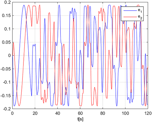
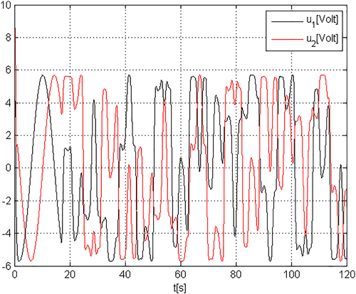
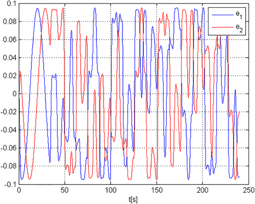
Assuming that the reference signals are the ones in Figure 8 and the disturbance is absent, the tracking errors are displayed in Figure 9, while the control voltages are shown in Figure 10. Figure 11 displays the obtained metal ring.
The maximum time constant
 is numerically calculated as
 whereas the estimate provided by using the provided Algorithm with Lemma 4 and N = 4 is equal to τc = 0.1026.
 (86)
(86)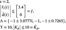 (87)
(87) (88)
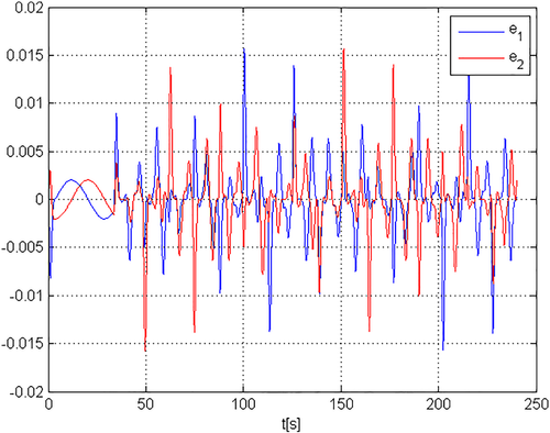
(88)Assuming that the references are shown in Figure 8 and the disturbance is absent, the tracking errors are displayed in Figure 12.
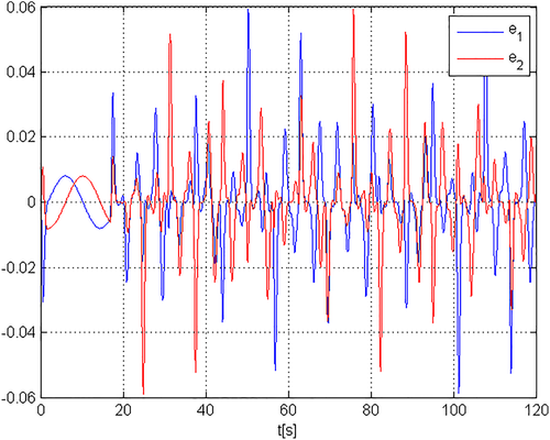
The maximum time constant
 is numerically calculated as
 whereas the estimate provided by using the provided Algorithm with Lemma 4 and N = 4 is equal to τc = 0.1031.
 (89)
(89)If the cutting velocity is halved (Figure 13), then the tracking errors for the controller 85 (v = 1) and the ones for the controller 88 (v = 2) are reported in Figures 14 and 15, respectively. Note that the obtained errors are respectively the half and one-fourth of those in the previous case, in accordance with Remark 8. Clearly, upon reducing the velocity and acceleration, the control signal also decreases, as well as the motor power.
 with a halved cutting velocity
To reduce the tracking errors or increase the cutting velocity without reducing the errors, it is possible to increase the size of the optimization parameter set ϒ. However, this approach may result in higher control signals.
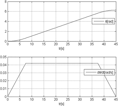
Example 3.Consider a milling machine composed of a Cartesian conveyor to move the working table along the directions X – Y and a planar robot with rotoidal joints to move the milling cutter C (see Figures 16 and 17).
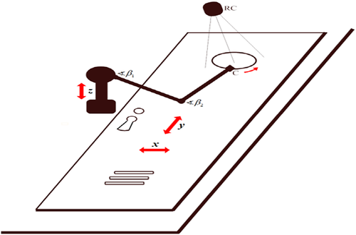
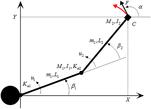
 (90)
(90) and
and
 is the vector of disturbance torques due to interaction of the milling cutter with a workpiece. If the working area is sufficiently bounded, the controller can be designed using the linearized model of the robot.
 (91)
(91) , ue = 0, and de = 0 is given by
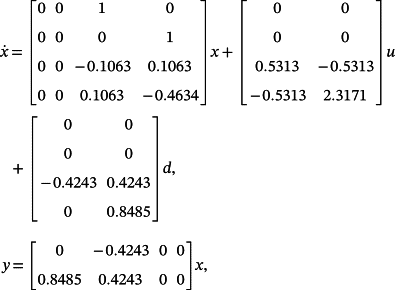 (92)
(92) (93)
(93)
Remark 14.Note that the designed controller is easy to realize, since it does not require the measurement of β (being Kβ = 0), and the measurement of e can be obtained with a robot camera if the reference r is depicted on the workpiece. Moreover, this controller is also robust against the measurement noises, due to the integral action included in the control law 95, and the fact that the reaction of the joints' velocity is inside of the control cycle which uses the tracking error.
 (97)
(97)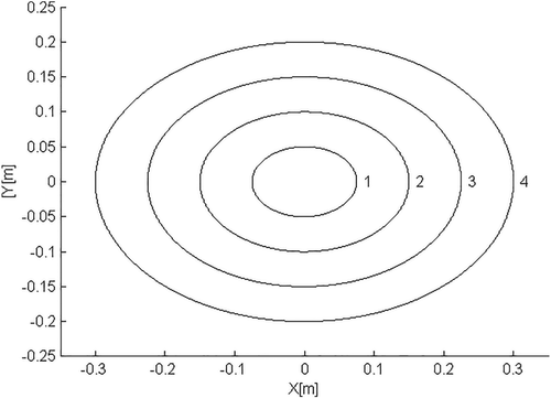

 the tracking error bounds are given by
 (98)
(98) (99)
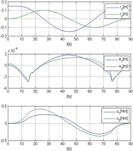
(99)The time histories of rx,ry, tracking errors ex,ey, and control torques u1,u2 are reported for i = 2 and controller 95, 96 in Figure 20.
Finally, for i = 2 and the controller 95, 96, if
 is affected by a measurement noise uniformly distributed in the interval
 and y is affected by a measurement noise uniformly distributed in the interval
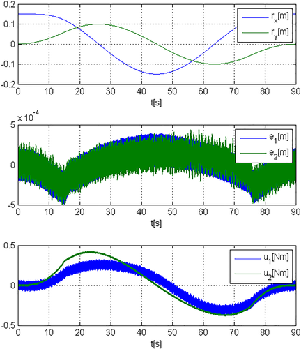
 , the tracking errors ex,ey and control torques u1,u2 are shown in Figure 21.
 and y affected by noises
8 CONCLUSIONS
In this paper, a broad class of LTI uncertain MIMO systems with bounded parametric uncertainties and/or affected by disturbances with bounded derivatives of order ν has been considered. The tracking problem has been systematically presented for generic sufficiently smooth reference signals, for instance, with bounded ν-th order derivatives. The employed majorant systems approach results in designing the state-feedback proportional-integral controllers of order v. The case of systems with additional bounded nonlinearities and/or not directly measurable states has been studied as well.
- uncertain LTI MIMO plants are considered generic;
- reference signals and/or disturbances are considered generic, with bounded v - th order derivatives
- the obtained results allow one to systematically design robust controllers for tracking generic reference signals with an acceptable precision, despite the presence of measurement noises;
- the proposed controllers avoid the derivative action causing realization problems, especially in the presence of measurement noises.
Finally, the obtained results have been validated by three examples: the first one is given to illustrate the proposed methodology, whereas the second and third examples deal with a metal-cutting problem for an industrial robot and a composite robot, such as a milling machine, to show practical advantages and effectiveness of the designed controller.
The ongoing research is conducted on extending the above results to some classes of uncertain LTI MIMO processes and/or other types of controllers, to design robust control laws guaranteeing pre-fixed maximum tracking errors, considering also the physical constraints of the control signals.
FUNDING INFORMATION
This work was supported by the Mobility Program of University of Naples Federico II, the Italian Ministry of Education, University and Research, and the Consejo Nacional de Ciencia y Tecnología.
AUTHORS' CONTRIBUTIONS
Laura Celentano: Conceptualization; Formal analysis; Funding acquisition; Methodology; Software; Supervision; Validation; Writing - original draft; Writing - review and editing. Michael Basin: Formal analysis; Funding acquisition; Supervision; Writing - original draft; Writing - review and editing. Mohammed Chadli: Supervision; Writing - original draft; Writing - review and editing.
Biographies

Laura Celentano (SM'19, M'04) received the Ph.D. degree in automation and computer science engineering (with major in automatic control and system analysis) from the University of Naples Federico II, Naples, Italy, in 2006. She has been an Assistant Professor of Automation and Control with the University of Naples Federico II, and a Professor of Fundamentals of Dynamical Systems, Modeling and Simulation, and Automation of Navigation Systems, since 2006. She has also taught classes at the University of Naples “Parthenope” and the Italian Air Force Academy, Naples.
She has taken an active part in activities co-funded by the European Union, the Italian Ministry of Education, University and Research, Region Campania, public and/or private corporations, and industrial companies. She is an author/reviewer for IEEE, ASME, ELSEVIER and AIP journals and conferences. Dr. Celentano has also been the Chair and an Organizer for conference sessions, also of Women in Control session. Currently, she is Associate Editor for the Journal of the Franklin Institute. She is Guest Editor for a special issue in Asian Journal of Control. She has authored and co-authored scientific and educational books, presented by the IEEE Control Systems Society and international experts. She is a science journalist and has cooperated with radio programs and journals on the dissemination of scientific matters. Her current research interests include the design of versatile, fast, precise, and robust control systems of linear and nonlinear uncertain systems; methods for the analysis of stability and for the stabilization of linear and nonlinear uncertain systems (as well as MIMO and discrete-time systems); modeling and control of rigid and flexible mechanical systems; multi-valued control design methodologies; modeling and control of aeronautical, naval, and structural systems; rescue and security robotics; and tele-monitoring/control systems.

Michael V. Basin (SM'07, M'95) received his Ph.D. degree in Physical and Mathematical Sciences with major in Automatic Control and System Analysis from the Moscow Aviation University (MAI) in 1992. He is currently Full Professor with the Autonomous University of Nuevo Leon, Mexico, and Leading Researcher with ITMO University, St. Petersburg, Russia. Starting from 1992, Dr. Basin published more than 300 research papers in international referred journals and conference proceedings. He is the author of the monograph “New Trends in Optimal Filtering and Control for Polynomial and Time-Delay Systems,” published by Springer. His works are cited more than 5,000 times (h index = 40). Dr. Basin has supervised 15 doctoral and 9 master's theses. He has served as the Editor-in-Chief and serves as the Senior Editor in Control of Journal of The Franklin Institute, a Technical Editor of IEEE/ASME Transactions on Mechatronics, an Associate Editor of Automatica, IEEE Transactions on Systems, Man and Cybernetics: Systems, IET-Control Theory and Applications, International Journal of Systems Science, Neural Networks. Dr. Basin was awarded a title of Highly Cited Researcher by Thomson Reuters, the publisher of Science Citation Index, in 2009; he is a regular member of the Mexican Academy of Sciences. His research interests include optimal filtering and control problems, stochastic systems, time-delay systems, identification, sliding mode control and variable structure systems.

Mohammed Chadli (Senior Member'99, IEEE) received the MScEng (DEA) from the Engineering School INSA-Lyon (1999), the PhD thesis in Automatic Control from the University of Lorraine (UL-CRAN) Nancy France in 2002 and his habilitation in 2011 at the University of Picardie Jules Verne (UPJV) Amiens, France. He was Lecturer and Assistant Professor at the “Institut National Polytechnique de Lorraine”-UL (2000–2004). Since 2004, he was Associate Professor at the UPJV and currently Full Professor at the University Paris-Saclay, Univ Evry, IBISC Lab., France. He was a visiting professorship at the TUO-Ostrava (Czech Rep.), UiA (Norway), SMU-Shanghai (2014–2017), NUAA-Nanjing (2018, 2019) and the University of Naples Federico II (Italy). Dr Chadli's research interests include fuzzy/LPV and switched systems, singular systems, robust control, fault detection and isolation (FDI), fault tolerant control (FTC) via LMI, SOS and Lyapunov methods. On the application side, he is mainly interested in automotive control and renewable energy. He is co-author of books and book chapters (Wiley, Springer, Hermes), and numerous articles published in international journals and conferences.
Dr. Chadli is a senior member of IEEE. He is also an Editor/Associate Editor/Editorial Board Member of several international journals, including the IEEE Transactions on Fuzzy Systems, Automatica, the IET Control Theory and Applications, the Franklin Institute Journal, Asian Journal of Control, etc. and was a Guest Editor for Special Issues in international journals.


