US employment exposure to domestic and foreign tariff changes under NAFTA
Editor in charge: Alessandro Bonanno
Abstract
Literature examining the effects of changes in trade agreements and import competition on US employment and wages has focused primarily on non-agricultural industries and changes in US import tariffs. We propose a method for measuring worker exposure to changes in agricultural tariffs using a newly developed county-level dataset of employment shares by crop and livestock type. We apply the method to examine the spatial concentration of US county-level employment-weighted exposure to changes in tariffs caused by the North American Free Trade Agreement (NAFTA). Results reveal noteworthy decreases in average US county-level crop and livestock employment exposure to Mexican import tariffs on US products. Findings also show spatial variation in US employment exposure to changes in Mexican import tariffs on US agricultural and non-agricultural goods. Changes in county-level employment exposure to US and Canadian import tariffs after NAFTA implementation are relatively minor given low initial tariff rates prior to the agreement.
There is renewed demand for economists to examine the efficiency and distributional implications of trade policies for labor markets and local economies. Globally, barriers to trade increased in recent years (Constantinescu et al., 2019). This includes increased tariffs from trade wars and barriers to the movement of people and goods implemented in response to COVID-19 (Beckman et al., 2021; Beckman & Countryman, 2021; World Trade Organization, 2020). Previous literature examines the effects of trade liberalization on employment and wages in non-agricultural industries of the United States (Autor et al., 2013, 2014; Hakobyan & McLaren, 2016). However, the lack of detailed analysis of agricultural sectors from this literature has important implications, especially for rural communities where agricultural exports are an important source of income (Zahniser et al., 2017). This paper proposes a method for measuring worker exposure to changes in agricultural tariffs using a newly developed county-level dataset of employment shares by crop and livestock1 type. We use this novel dataset to examine US worker exposure to domestic and foreign import tariff changes that resulted from NAFTA. We differentiate crop, livestock, and non-agricultural tariff changes and compare the magnitude of the employment-weighted changes across these sectors. Finally, we illustrate the spatial distribution of US worker exposure to changes in both agricultural and non-agricultural tariffs.
Neoclassical economic theory assumes that labor will migrate across industries in response to trade liberalization, from industries or locations where the country does not have a comparative advantage to industries or locations where the country does. However, empirical studies show that there are high frictions to labor mobility following changes in trade policy or exposure to import competition (Autor et al., 2013, 2014; Dix-Carneiro & Kovak, 2015, 2017; Hakobyan & McLaren, 2016; Topalova, 2007, 2010). Autor et al. (2014) find heterogeneous effects of import competition on worker mobility in the United States across workers' initial skills and wages. Low-wage workers initially employed in industries that experienced high import competition tended to migrate to firms within the same sector, thus experiencing multiple employment disruptions as import competition increased over time. In contrast, high-wage workers were better able to migrate to higher performing industries over the long run, experienced greater wage growth, and were less likely to take public disability benefits than low-wage workers. These findings show that trade liberalization can sometimes exacerbate economic inequalities. Furthermore, labor market impacts of trade policies can be persistent. Wages and formal sector employment were still depressed in industries and locations exposed to greater import competition more than 20 years after Brazil cut import tariffs in a large-scale trade liberalization effort (Dix-Carneiro & Kovak, 2017). Additional research to understand how trade liberalization or protectionist policies implemented by a country or its trade partners affect labor markets in urban and rural communities across agricultural and non-agricultural sectors is imperative for informing policy, enhancing labor market opportunities, and anticipating changes in labor migration.
Previous literature examining the effects of NAFTA on worker wages in the United States shows that NAFTA depressed wages in industries that experienced large declines in tariff protection from 1990 to 2000 (Hakobyan & McLaren, 2016). Service sector workers also had depressed wages if they were employed in locations where a large share of the workforce was employed in industries that had large declines in US import tariffs during NAFTA. However, the agricultural sector was deliberately excluded from the analysis of Hakobyan and McLaren (2016) due to lack of detailed data on labor use by crop and location. While their findings are robust to the inclusion of the aggregate agricultural industry, agricultural tariffs changed substantially during NAFTA and this may have had unintended consequences across agricultural sectors. For example, the sector labeled “canned, frozen, and preserved fruits and vegetables” was the third most protected industry in the United States in 1990.2 After adjusting for Mexico's Revealed Comparative Advantage (RCA)3 in production of goods in each industry, it drops to the fifth most protected industry, and agricultural crop production becomes the eighth most protected industry (Hakobyan & McLaren, 2016).
In rural communities, where agriculture is a more dominant employer, changes in agricultural tariffs could have important labor market implications that are not fully understood when only controlling for the effects of aggregate agricultural labor exposure to tariffs. Crop aggregations mask important variation in the magnitude of tariff changes and labor intensity across individual crops. Since the United States is a major exporter of agricultural goods, changes in foreign tariffs on US goods could have important labor market effects in the United States. Even though some crops lost protection with implementation of NAFTA, others gained access to foreign markets. Therefore, it is important to consider the labor market effects of reductions in both domestic and foreign import tariffs.
Little research has been devoted to understanding the effects of trade liberalization on employment and wages in rural communities of developed countries with a large agricultural presence. One notable exception is Autor et al. (2024), who show that Chinese import tariffs imposed on US agricultural goods during the 2018–2019 trade war negatively affected US agricultural employment while US worker exposure to US import tariffs on non-agricultural goods had no sizeable effect. The authors measure US employment by sector using 6-digit North American Industry Classification System (NAICS) codes in the Quarterly Census of Employment and Wages (QCEW) and impute employment by sector and commuting zones using higher aggregations of industries or geographic locations when the QCEW data are suppressed. Furthermore, He (2020) uses farm employment data from QCEW and the US Bureau of Economic Analysis to estimate the impact of agricultural exports on local employment. He (2020) finds that a 1% increase in agricultural exports increases farm employment by 0.302% and has no statistically significant impact on nonfarm labor.
We provide an alternative method to measuring crop- and livestock-specific employment exposure to both domestic and foreign tariffs at detailed geographic levels by using precise crop and livestock (including animal products) classifications in the US Census of Agriculture. Our method is less reliant on QCEW data, which prior to 2004, did not report the number of establishments in suppressed industry observations and prior to 2001, did not distinguish between observations that were suppressed versus zero. The count of establishments in industries with suppressed labor observations is critical to the imputation methods of Autor et al. (2024), making their methods impossible to replicate in years prior to 2004. There may be other advantages to our alternative agricultural employment measure. For instance, our method reduces concerns of underreporting of unauthorized immigrant agricultural workers in the QCEW data. Finally, our method assigns agricultural workers of different contract types, including employees of farm labor contractors (FLCs), to specific crops. For these reasons, our method provides some advantages, especially for examining labor exposure to shocks prior to 2004.
We create a unique dataset that combines trade data detailed to the 6-digit Harmonized System (HS) product code with county-level acreage and production data for specific crops and livestock in the US Census of Agriculture, labor inputs by crop from crop enterprise budgets, and wage and employment data from the QCEW. We measure county employment exposure to changes in tariffs using methods similar to Topalova (2007, 2010), additionally weighting tariffs by the trade partner's RCA as in Hakobyan and McLaren (2016). We show that, on average, the decrease in US tariff protection under NAFTA was much smaller in magnitude than the decrease in tariffs that Mexico imposed on imports of US goods. Furthermore, the decrease in Mexican import tariffs on crops and livestock was larger in magnitude than its decrease in non-agricultural import tariffs. Canadian import tariffs on US goods were relatively low prior to NAFTA, so the magnitude of changes was much less than for Mexican import tariffs. Finally, we show that in many counties, the employment-weighted workforce exposure to reduced foreign import tariffs on US crops was larger in magnitude than changes in workforce exposure to reductions in US or foreign import tariffs on non-agricultural goods following the roll-out of NAFTA. The geographic spread and magnitude of changes in worker exposure to foreign import tariffs on US goods varied substantially across crops, livestock, and non-agricultural goods. Our findings illustrate the importance of investigating labor market exposure to tariff changes in each of these sectors distinctly.
Our focus on the agricultural sector is an important distinction from previous literature since the United States was a net exporter of agricultural products during the roll-out of NAFTA, and employment and wages in agricultural communities might benefit from reduced foreign tariffs on US goods. Although previous literature shows that employment and wages declined following the roll-out of NAFTA in locations where labor exposure to reduced US tariffs on non-agricultural industries was greater (Hakobyan & McLaren, 2016), to understand the full implications of NAFTA and other trade agreements, empirical investigation needs to account for changes in workforce exposure to both US and foreign import tariffs. In this paper, we develop data and methods to more accurately measure employment exposure to tariff changes in the agricultural sector and further explore how labor exposure to changes in US and foreign import tariffs across crop, livestock, and non-agricultural sectors compared during the roll-out of NAFTA. Our findings suggest that connections between tariffs and labor might be more complex than previous literature implies, and therefore merit further exploration.
This paper proceeds as follows. In the next section, we review the relevant literature. Next, we describe the data. In the following section, we calculate county employment exposure to domestic and foreign import tariffs. Then, we illustrate spatial variation in changes in county exposure to domestic and foreign import tariffs by sector during NAFTA implementation. We discuss potential policy implications of sector-specific labor exposure to trade policy, and lastly, we conclude.
RELATED LITERATURE
This section knits together literature on the distinct characteristics of agricultural and rural labor markets in the United States, the labor market effects of domestic and foreign policy changes, and the medium- to long-term effects of NAFTA and other trade agreements. Although it is well understood that NAFTA had important implications for the US agricultural sector (Zahniser et al., 2015; Zahniser & Link, 2002; Zhao et al., 2020), we know of no other analyses that measure worker exposure to changes in foreign and domestic import tariffs during NAFTA using detailed employment data disaggregated across space (by county) and by crop and livestock types. Nevertheless, Autor et al. (2024) show that the agricultural sector's exposure to changes in foreign import tariffs can have important implications for rural employment, and detailed measures of employment by crop type are essential for careful analysis of the labor market effects of trade policies.
Agricultural and rural labor markets are distinct from those in metro areas of the United States, and changes in employment opportunities can have a myriad of consequences that are difficult to predict. For example, decreased employment and wages are associated with increased opioid overdoses within metro and nonmetro counties of the United States. Betz and Jones (2018) find differential effects by skill level, gender, and race, which suggests that both the number and types of jobs available in a region are important. Agricultural employment could also have important implications for other social welfare outcomes. Increased seasonal fruit, vegetable, and horticultural employment within US counties is associated with a significant decrease in property crime rates, even after controlling for county-by-year fixed effects (Charlton et al., 2022). Increased economic opportunities likely deter crime during labor-intensive seasons of farm production, even if more people migrate into the region. This is consistent with evidence that unemployment and wages influence crime rates (Gould et al., 2002; Yamada et al., 1993), though James and Smith (2017) find that an economic boom can also increase crime rates. These findings demonstrate the importance of understanding how rural and urban labor markets are exposed to domestic and foreign trade policies.
Agricultural labor markets have important location and time dimensions, which are often determined by conditions like weather (Fisher & Knutson, 2013). Overall employment rates might consequently mask important distinctions in agricultural labor markets. Farm workers have become less migratory over time (Fan et al., 2015). Fan et al. (2015) find that from 1999 to 2009, the share of crop workers who migrated decreased by more than 60%. These trends have important implications for the ability of agricultural labor markets to adjust quickly and smoothly to changes in labor demand such as following changes in foreign and domestic trade policies. The use of FLCs to match workers to temporary or seasonal jobs, thus reducing labor market frictions, is relatively common in California and Florida where labor-intensive specialty crops are grown in greater concentrations, but less common in other regions of the United States (Fisher & Knutson, 2013). Although detailed data on crop-specific employment are sparse, research on farm labor markets needs to account for important variation across crops and where they are grown since workers are not perfectly mobile.
There is evidence that farm workers do not immediately migrate to other sectors as relative wages in other sectors rise, consistent with the notion that workers associate an option value with remaining in their current sector of work (Önel & Goodwin, 2014). However, Richards and Patterson (1998) show that workers migrate more rapidly from agricultural to non-agricultural sectors than the reverse. Following NAFTA, Boucher et al. (2007) find that migration from rural Mexico to US farms increased, but there has been little investigation of agricultural worker exposure to changes in foreign and domestic tariffs.
While several studies investigate the effects of import competition on US employment, it is important to consider both worker exposure to domestic import tariffs and exposure to foreign import tariffs levied on US exports. Feenstra et al. (2019) investigate overall state-level employment effects of import competition from China and find that export expansion creates employment opportunities that offset jobs lost in import-competing industries. However, Autor et al. (2016) and Kondo (2018) find unequal distribution of employment effects. They find that the magnitude of the negative effect on workers in import-competing industries was larger than the magnitude of the positive employment effects for workers in export-oriented industries. While these studies provide insights into overall employment effects of trade exposure, agriculture is either not accounted for or is aggregated into one combined employment sector. Furthermore, studies show that NAFTA-related tariff reform for agricultural products led to trade creation that exceeds trade diversion (Burfisher et al., 2001; Kennedy & Rosson, 2002), highlighting the need to explicitly account for changes in agricultural and non-agricultural tariffs faced by both US imports and exports when considering rural employment exposure to trade protection.
Related to the impacts of tariff policies, the literature has also explored the rural development and labor market implications of exports. For example, USDA multipliers suggest that agricultural exports have positive effects in rural areas for both agricultural and non-agricultural sectors (He, 2020). Existing empirical studies confirm that agricultural exports benefit farmers and owners of farm assets (Kilkenny & Partridge, 2009; Weber et al., 2015), but they find limited evidence of spillovers into non-agricultural sectors. Consistent with this, He (2020) finds that agricultural exports increase farm employment but do not lead to significant increases in non-farm employment.
Given the unique features of US agricultural labor markets, NAFTA likely had distinct effects on employment and wages that vary across US crops, livestock, and regions of employment. Studies that aggregate agricultural employment (e.g., Hakobyan & McLaren, 2016) mask this variation. Furthermore, research that accounts for the effects of improved access to foreign markets through the reduction of foreign import tariffs on US goods is essential. Researchers have measured the effects of US tariff changes on employment and wages in Canada and Mexico using detailed geographic employment data (Chiquiar, 2008; Feliciano, 2001; Kovak & Morrow, 2022). However, literature measuring the effects of changes in foreign import tariffs on US employment and economic activity (e.g., Burfisher et al., 2001; Congress of the United States Congressional Budget Office, 2003) during NAFTA do not closely examine spatial variation in labor market exposure.
We contribute to the existing literature on labor markets and trade policy by examining US agricultural and non-agricultural employment exposure to changes in US and foreign import tariffs during a major trade agreement that began in the 1990s. We use a method that accounts for the importance of specific commodities within local agricultural labor markets. One of the few papers that investigates agricultural employment exposure to changes in trade policy in a developed country is Autor et al. (2024), which examines the effects of the United States–China 2018 trade war on agricultural employment. We build on this literature by developing an alternative measure of agricultural employment by crop and livestock type. Our measure offers several advantages, particularly for measuring crop-specific employment shocks prior to 2004. First, the method described in Autor et al. (2024) relies on information about the number of suppressed observations. In 2001 and following years, QCEW began reporting if missing employment data were the result of zero employment or because of data suppression required to protect the privacy of individual firms. Prior to 2001, researchers do not know if missing employment is because of suppression or because of zero employment. Furthermore, in 2004, QCEW began recording the number of establishments even when all other data for the county-NAICS or state-NAICS pair are suppressed. Autor et al. (2024) use these establishment counts to more precisely allocate employment across missing values, but this is only possible in 2004 and later. Given these limitations in the QCEW data prior to 2001 and 2004, we would not be able to estimate base year tariff exposure prior to NAFTA using the methods employed by Autor et al. (2024).
Second, QCEW only records employment for workers who are reported for Unemployment Insurance, and there is concern that many agricultural workers might be omitted. A large share of crop workers is unauthorized (estimated around 50 percent in many years in the National Agricultural Workers Survey [NAWS]). While many unauthorized immigrants use borrowed Social Security numbers and would thus be counted as any other worker in Unemployment Insurance, we do not know how many might be omitted or whether omission varies across crop types. Furthermore, small farms are not required under federal mandate to report employment.4 Our methods for measuring labor hours by crop type mitigate concerns related to the misreporting of unauthorized workers in the QCEW and underreporting by small farms.
Finally, using crop enterprise budgets provides us with slightly more disaggregated crop-specific information and does not distinguish employees of FLCs but assigns these workers to specific crops like any other worker. In the QCEW, FLCs have a NAICS industry code (NAICS 115115) and it is unknown what crops they work on. Since FLCs accounted for more than 14% of the crop workforce in 2019 and were the fastest growing share of farm workers (Costa & Martin, 2020), and in 1990, they accounted for about one-third of crop employees in California (Martin & Taylor, 1990), it is important to include FLC workers in analysis of agricultural employment, especially in states like Florida and California where FLCs are more prevalent. Our methods also disaggregate other NAICS codes that cluster several crops. For example, NAICS codes combine many tree nut crops into a single sector (111335) while we treat different tree nut crops (e.g., pistachios, almonds, walnuts) separately.
This analysis provides many important contributions to the trade and agricultural labor literature. Importantly, we compare employment exposure to both US and foreign import tariff changes during NAFTA, which was a notable trade agreement in that it eliminated most barriers to trade between three countries and remained in effect for 26 years until it was replaced by the US-Mexico-Canada Agreement in 2020. Understanding how worker exposure to tariff changes during the roll-out of NAFTA varied across sectors and geographic locations has important implications for learning about and anticipating the potential social impacts of this and future trade policies.
DATA
We create a unique dataset of county-level tariff exposure based on the number of employees in different sectors. We combine data from the World Integrated Trade Solution (WITS) database, CEPII5 MAcMap HS6 (Guimbard et al., 2012), the US Agricultural Census, the Bureau of Labor Statistics QCEW, and farm-level crop enterprise budgets published by various US universities. We create the first national dataset to our knowledge with county employment shares by individual crops that do not depend on employer-provided Unemployment Insurance reports as in the QCEW. We combine these data with employment shares in non-agricultural and livestock products, and US, Canadian, and Mexican import tariffs by product and year.
Trade and tariff data construction
We obtain pre-NAFTA trade and tariff data from the WITS database, which accesses major international trade databases—the United Nations (UN) Comtrade database for trade and the United Nations Conference on Trade and Development (UNCTAD) Trade Analysis Information System (TRAINS) database for tariffs. We employ tariff data for the post-NAFTA period from Guimbard et al. (2012), which provides applied rates of protection in 2010. Applied rates from this source were first available in 2001, and we use tariff data from 2010 because NAFTA tariff changes were fully rolled out by 2010 (Zahniser et al., 2015).
We use the WITS database to construct pre-NAFTA tariff rates. To account for missing observations for pre-NAFTA tariff data, we include the lowest recorded tariff rate from 1991 to 1994 in the WITS database. For Canada, the only available tariff data were from 1993, for Mexico, data are only available from 1991, and for the United States, tariff data were available in 1992 and 1993. From the WITS database, We also use annual bilateral trade flows at the HS 6 product level in 1992. We use the HS6 product code level because we can more precisely match tariffs to specific crops and livestock. We use bilateral import and export trade values in nominal US dollars from Canada, Mexico, the United States, and the rest of the world (ROW). We merge the trade flow data with bilaterally applied import tariffs at the HS6 level.
For some products, no tariff is reported in the pre-NAFTA period, and a positive tariff is reported in 2010. This occurs most frequently for Canadian livestock tariffs (10.96% of livestock product codes imported from the United States) and for US livestock tariffs (5.93% of livestock product codes imported from Mexico or Canada). Fewer than 1% of product codes in crops and livestock showed an increase in US import tariffs. No crops and fewer than 1% of non-agricultural products had an increase in Canadian tariffs on imports from the United States. No livestock products, 3.5% of crop products, and fewer than 1% of non-agricultural products had an increase in Mexican tariffs on imports from the United States. Since the increase in tariffs appears to be the result of missing tariff observations pre-NAFTA, and the World Trade Organization (WTO) encouraged countries to convert nontariff measures (NTMs) to tariffs during this time period (Daly & Kuwahara, 1998), we attribute the increase in tariffs to either missing data or tariffication of NTMs rather than an outcome of NAFTA. NAFTA was implemented to decrease trade barriers, so we replace tariff increases with zero change in tariffs between our pre-NAFTA and post-NAFTA observations.
In Figure 1, we plot the weighted mean tariffs by sector and trade partner pairs for pre- and post-NAFTA periods. While the United States decreased import tariffs on Mexican non-agricultural goods by about 2 percentage points on average, this is not nearly as large as the decrease in Mexican import tariffs on US goods. In each sector, mean weighted Mexican import tariffs decreased by more than 10 percentage points. Changes in Canadian import tariffs on the United States and US tariffs on Canada were relatively small in magnitude.6

Labor data construction
Lacking detailed employment data by crop and livestock type, we calculate crop and livestock employment by combining data from numerous sources detailed in Appendix S1. To find employment by crop of type , we take detailed acreage data by crop from the 1992 US Census of Agriculture. Although the Census of Agriculture does not record workers per crop, we can estimate total labor hours per crop in each county by multiplying acreage for each crop in the county by the labor hours per acre required to produce each crop for a representative farm. We take hours per acre from crop enterprise budgets published at various universities.7
One of the challenges in using crop enterprise budgets to estimate the labor intensity of crop production is that many tasks performed on farm are hired through custom operations, and the budgets do not always contain detailed labor input data. We spoke with authors of UC Davis budgets to approximate percentages of costs for agricultural production activities like discing or spraying that can be attributed to labor, so that we can include these activities in total labor inputs even when they are written only as total custom line items. To the extent that these services have similar production technologies across the country and across crops, the estimates provided by these authors are a reasonable proxy for the labor per acre in these services. This represents an improvement over assuming that the labor cost share of custom contracted activities in crop production is 0.
We note that our method uses crop enterprise budgets from the 2010s and 2020s, but that tariff changes under NAFTA occurred in the 1990s and 2000s. If crop labor amounts per acre have changed significantly over time in different ways for different crops (e.g., through mechanization), our estimates may contain bias. However, the USDA Economic Research Service8 finds that mechanization slowed or even reversed as of the 1990s in the United States. Consistent with this, Alvarez-Cuadrado et al. (2017) examine shifts in capital–labor ratios in agriculture. Finally, Hamilton et al. (2022) show that profit maximizing firms in a labor market that is not perfectly competitive will be slow to adopt mechanical aids that complement labor because this would increase the demand for labor and put upward pressure on wages. They find that, despite available mechanical technologies that enhance labor productivity in strawberry production, mechanical adoption has been slow. They suggest that this explains why the productivity gap in US agriculture has been persistent, and why technological advances have not “pushed” workers out of agriculture. Thus, evidence suggests that employer market power in the agricultural sector has disincentivized technology adoption and stabilized farm employment in some labor-intensive crops, including strawberries.
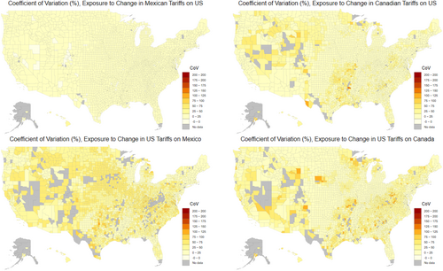
There are other potential sources of bias in our estimates of crop employment shares. For example, crop enterprise budgets are based on a subsample of farms that are not necessarily representative of each crop industry as a whole. To mitigate concerns about representativeness, we collect as many budgets as possible and use average labor intensities. This diminishes the importance of any one budget in influencing our results. Next, there could be geographic variation in labor intensities that our method misses. We explore if under- or over-estimates of crop labor per acre influence our results by performing a Monte Carlo analysis described in Appendix B. By randomly selecting from a distribution of labor intensities (independent by crop), we quantify how sensitive our estimates are to the estimated crop labor intensity. Results in Figure B1 show how crop employment shares at the county level vary by US census region. After taking 500 random draws of crop labor hours per acre, independently for each crop, we calculate crop employment-weighted mean tariffs in each county and calculate the coefficient of variation across all simulations. We plot the coefficient of variation by county in Figure B2. The coefficients of variation are relatively small across the nation for all trade partner pairs. Finally, we present a series of .gifs in Figures B3-B6 showing our main results for a random sample of 25 of the 500 Monte Carlo iterations used in the sensitivity analysis. While small variations exist, it becomes clear that the regions that are exposed to tariff changes remain consistent across iterations.
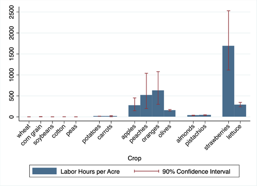
Even allowing for variation in the labor required to produce each crop, we obtain a robust estimate of the relative intensity of different crops. This leads to the overall robustness of our main results to the draw of specific crop labor intensities. In Figure B7, we present the mean and 90% confidence interval for labor hours per acre for 15 crops. The method clearly distinguishes between labor-intensive crops like strawberries or oranges, highly mechanized crops like wheat, soy, or corn, and a range of crops in between, like almonds (mostly mechanized) and lettuce (relatively quick to hand-harvest compared with strawberries and most orchard fruits).
This approach to measuring labor use by crop does not rely on imputation of QCEW data as described in Autor et al. (2024). While measuring crop-specific labor intensity can be challenging, it offers an alternative approach to measuring agricultural labor's exposure to tariff changes. In the context of estimating NAFTA impacts, an alternative to QCEW imputation has several advantages as already described in Related literature.
For livestock employment shares, since we lack proxies of employment per animal, we approximate livestock employment shares with the share of total livestock value in the county for each animal (cattle, sheep, dairy, hogs, poultry, mink, and fish/aquaculture by type) in the 1992 Census of Agriculture.
For the non-agricultural sector, we use employment data from the QCEW. The QCEW includes data for all workers who worked or received pay during the pay period including the 12th day of the month and who were covered by the state Unemployment Insurance laws (and federal workers covered by the Unemployment Compensation for Federal Employees program). We use employment by 3-digit NAICS industry codes, including forestry and logging (NAICS 113) but excluding crop production (NAICS 111), support activities for crop production (NAICS 1151), livestock production (NAICS 112), fishing, hunting and trapping (NAICS 114), support activities for animal production (NAICS 1152), food manufacturing (NAICS 311), and beverage and tobacco product manufacturing (NAICS 312). Since there is suppression in the QCEW data, and we do not know whether missing values are suppressed or zeroes, we fill in missing industries where possible. To do so, we sum employment by industry NAICS across all counties in each state and take the difference between this sum and the state-reported employment by industry. We then distribute this difference evenly across all counties with missing data for that industry.
In order to merge employment share data with trade and tariff data, we map HS codes to non-agricultural NAICS 3-digit codes and map HS codes to crops and livestock. To perform this mapping, we searched for all HS codes that contained the name of the crop or livestock type and determined whether the product was sufficiently processed to be considered a non-agricultural product. Since we expect tariffs on minimally processed goods to impact farmers, we map goods with some processing to crop and livestock sectors. For example, an import tariff on beef affects not only meat processing facilities but also feedlot and cow-calf operations in other locations. Generally, we map fresh, frozen, canned, and juiced products to fruit and vegetable production; we map flours, seeds, and roasted cereals to grain production; we map live animals, fresh and frozen meat, raw or tanned skins, and wool (carted and uncarted) to livestock production; and sweetened and unsweetened milks and creams, spreads, and cheeses to dairy livestock production. For illustration, the HS code mapping for tomatoes is recorded in Table 1. We include a table of all HS code mappings to all crop and livestock products in the Table S1.
| HS code | Definition |
|---|---|
| 70200 | Vegetables; tomatoes, fresh or chilled |
| 200210 | Vegetable preparations; tomatoes, whole or in pieces, prepared or preserved otherwise than by vinegar or acetic acid |
| 200290 | Vegetable preparations; tomatoes (other than whole or in pieces) prepared or preserved otherwise than by vinegar or acetic acid |
| 200950 | Juice; tomato, unfermented, not containing added spirit, whether or not containing added sugar or other sweetening matter |
| 210320 | Sauces; tomato ketchup and other tomato sauces |
CALCULATING COUNTY SECTOR EMPLOYMENT EXPOSURE TO DOMESTIC AND FOREIGN IMPORT TARIFFS
CHANGES IN COUNTY IMPORT TARIFF EXPOSURE DURING NAFTA IMPLEMENTATION
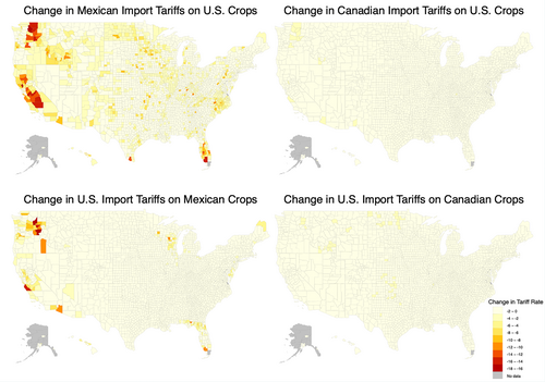
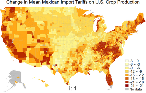
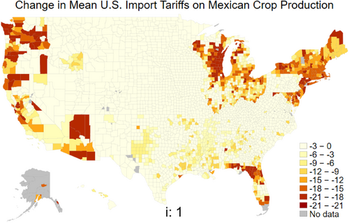
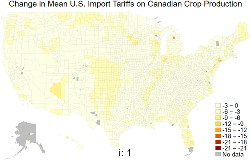
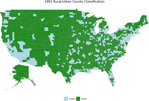
Figure 2 shows the county-specific changes in employment-weighted mean exposure to tariffs that Mexico and Canada imposed on imports of US crops and lightly processed related goods and changes in tariffs that the United States imposed on crop imports from Mexico and Canada. There were large reductions in average crop employment exposure to import tariffs imposed by Mexico across many rural US counties (see Figure C1 for a map of US counties by rural/urban status). Numerous metro areas were also exposed to large changes in Mexican import tariffs, especially those located in areas that produce lots of specialty crops like fruits, vegetables, and tobacco (for example, southern California and parts of the Northeast; see Figure E2). Reductions in exposure to Canadian import tariffs were relatively small in magnitude. A few regions that mostly specialize in vegetable production were exposed to relatively large declines in US tariffs on crop imports from Mexico.
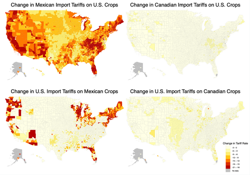
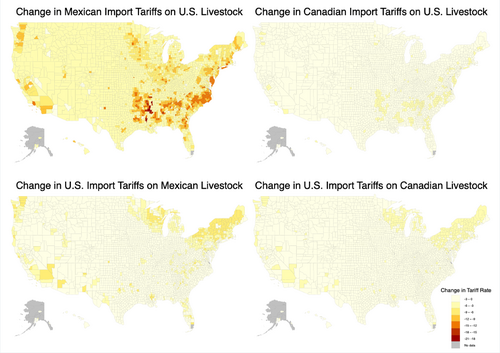
Figure 3 shows the county-specific changes in employment-weighted mean tariffs that Mexico and Canada imposed on imports of US livestock and animal products and that the United States imposed on imports of livestock and animal products from Mexico and Canada. Again, the largest change in exposure comes from decreases in Mexican import tariffs on US products. Major hog- and poultry-producing counties were exposed to relatively large declines in Mexican import tariffs on US livestock (see Figure A2). Dairy producing counties were largely exposed to decreases in US tariffs on imports of livestock and animal products from Mexico and to a lesser extent from Canada. Exposure to changes in Canadian import tariffs on US livestock was relatively small throughout the United States.
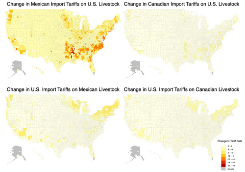
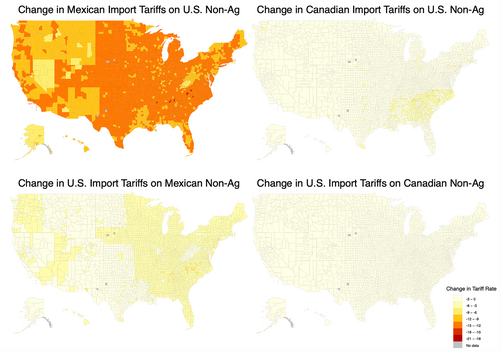
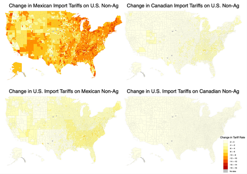
Figure 4 shows the county-specific changes in employment-weighted mean exposure to tariffs that Mexico and Canada imposed on imports of US non-agricultural goods and employment-weighted tariffs that the United States imposed on non-agricultural imports from Mexico and Canada. Exposure to changes in Mexican import tariffs on US non-agricultural goods is widespread, though there is some spatial variation. Previous literature has focused on changes in employment exposure to changes in US tariffs on imports from Mexico rather than exposure to declines in Mexican import tariffs on US non-agricultural goods (Hakobyan & McLaren, 2016). However, workers in non-agricultural industries potentially benefited from improved access to export markets.
To examine how labor exposure to tariff changes relates to the locations of specific crop and livestock industries, we map shares of county crop and livestock employment by crop and livestock type in Figures E1-E4. We find that counties where crop workers were exposed to the largest changes in tariffs during NAFTA were counties that specialized in the production of fruits, vegetables, and tobacco. Although the United States is a major exporter of field crops like corn, soybeans, and wheat, the tariff changes for these crops was relatively smaller than for many of the specialty crops, and we find that counties with large acreage of field crops were exposed to relatively small changes in crop tariffs. Changes in average tariff rates by crop are included in Figures E5 and E6.
Labor sector exposure to tariff changes as a share of total county employment
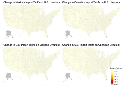
We map crop, livestock, and non-agricultural employment exposure to tariff changes weighted by share of total employment in Figures 5-7.9 Crop employment is a substantial share of total employment in very rural counties and counties that specialize in the production of labor-intensive fruits and vegetables, so we still observe that labor exposure to changes in crop tariffs weighted by share of total employment was large (a change of more than 15 percentage points in the tariff rate for some counties). Counties exposed to large crop tariff changes after weighting by share of total employment were primarily located in California, Washington, and Florida, but there was noticeable exposure to declines in Mexican import tariffs on US crops in counties dispersed across the country. These highly exposed counties mostly produce labor-intensive crops, such as fruits and vegetables. Livestock tends to be less labor-intensive on average and constitutes a more substantial share of employment only in very rural counties, so we observe few counties where the change in livestock tariff rates weighted by industry share of total employment in the county was larger than 3 percent. Non-agricultural labor exposure to changes in Mexican import tariffs on US products are more concentrated in the Eastern United States once we scale using non-agricultural labor's share of total county employment.
DISCUSSION AND POLICY IMPLICATIONS
Labor exposure to agricultural and non-agricultural tariff changes from NAFTA has several important lessons for policy moving forward. First, our work contributes directly to current US trade policy discussions. Politicians from both major US political parties have proposed increased import tariffs to protect domestic industries. Our work demonstrates that rising barriers to trade likely have differential effects across regions of the United States and sectors of the economy. While Hakobyan and McLaren (2016) focus on the domestic impacts of lowering US import tariffs, our work shows that US worker exposure to decreases in foreign import tariffs on US export products differed substantially across sectors of work and geographic location. Trade theory would predict that increases in United States' access to foreign export markets should increase demand for labor, thus putting upward pressure on employment and wages, even as decreases in US tariffs on imports during NAFTA implementation put downward pressure on employment and wages. Our findings suggest that the increased worker exposure to foreign trade policy was substantial, and further investigation is needed to determine to what extent the reduction in tariffs that Mexico and Canada imposed on the United States affected US employment and wages by sector and geographic location. The lessons from this and related work may be particularly important for predicting the impacts on labor of implementing higher import tariffs in the United States if other countries respond by also increasing protection.
Our work also has implications for agricultural labor specifically, which has been largely overlooked in previous literature. In regions with high employment in agriculture, tariff changes in other countries may have large impacts since the United States is a major exporter of agricultural goods. For example, producers in some regions of the United States were negatively impacted by Chinese tariff increases on US agricultural products (e.g., soybeans) in 2018 (Janzen & Hendricks, 2020). The federal government recognized the losses these tariffs imposed on the agricultural sector, but compensation payments (e.g., through the Market Facilitation Program) went to farm operators and may not reach agricultural workers who would also be impacted by the change in tariffs. Effects on agricultural labor fall on relatively poor households. This is evidenced by rising poverty rates as farm employment rose within US counties between 1980 and 1990 (Martin & Taylor, 2003).
Agricultural worker exposure to foreign tariffs documented in this paper also suggests that there may be an underappreciated linkage between trade policy and immigration policy. Higher foreign tariffs on US agricultural products may reduce the demand for agricultural labor and change the demand for immigrant workers across sectors, which could have important implications for rural economic outcomes, including poverty (Martin & Taylor, 2003). Future work is warranted to better understand how trade policy changes the sector and location in which individuals work. Further exploration could also test for crop-specific responses to foreign tariffs. The potential to focus on workers instead of counties highlights many interesting questions regarding the distributional effects of changes in trade policy exposure.
CONCLUSION
While the field of economics consistently demonstrates that workers are not perfectly mobile across industries or geographic space (Autor et al., 2013, 2014; Dix-Carneiro & Kovak, 2015, 2017; Hakobyan & McLaren, 2016; Topalova, 2007, 2010), there has been little research on US agricultural worker exposure to trade liberalization or protectionism. This can be especially important in rural communities with a large agricultural share of employment. Although the share of the US population employed in agriculture and related industries is relatively small (10.4% of US employment in 2022; USDA Economic Research Service, 2023), agriculture remains an important part of many rural communities. We find that changes in foreign tariffs on US products were large relative to changes in US tariffs on imports. This suggests that research should consider both exposure to tariffs on imports that increase competition in domestic markets and exposure to import tariffs in export markets that affect competitiveness in foreign markets.
Finally, we show that employment-weighted exposure to reduced Mexican import tariffs on US crop and livestock sectors was particularly large in several regions of the country. Given the relatively large declines in foreign import tariffs that US crop and livestock workers were exposed to, NAFTA might have benefited many industries and workers in nearby locations if there were substantial spillovers. This mechanism remains underexplored in the literature that has focused primarily on losses in non-agricultural employment protection from US tariff reductions on imports and merits further empirical investigation.
It may also be the case that individual workers are part of households with labor that is diversified across multiple sectors. Off-farm labor has been shown to have a wide range of effects on farm household outcomes in the United States (e.g., Mishra & Chang, 2012). Working off farm can mitigate agricultural risk (Bubela, 2016). In terms of how this affects our measure of labor exposure to tariffs, our estimate is based on labor hours by crop and sector and does not distinguish between labor within the same or different households. It also does not distinguish between management and hired labor. If a household member works in both crop farming and non-agricultural sectors, the labor that household provides could be counted in both sectors. In response to a tariff change, households could reallocate labor from industries facing relatively high tariffs to industries with lower tariffs. Further, diversified households may be exposed differently from labor (e.g., with some members benefiting from tariffs and others benefiting from more international trade). This suggests an avenue for future work to quantify how households rather than employment sectors are exposed to tariff changes.
There is much yet to investigate regarding the effects of agricultural trade and tariff changes on employment and wages. This paper develops crop- and livestock-specific employment weights and calls for future work to explore changes in tariff exposure to NAFTA and other trade policies. Employment weights can be used in analyses investigating a wide range of impacts on agricultural labor, ranging from specific crop mechanization to trade wars and climate change. Future work can examine the relative strengths and weaknesses of our method and using QCEW data to measure exposure to trade policies (Autor et al., 2024). Overall, measuring sector-specific employment exposure to trade policy enables timely future investigation connecting crop- and livestock-specific natural and market-driven shocks to employment and wage outcomes across US counties.
ACKNOWLEDGMENTS
We are grateful to Grace Gilbreth, Laura Sikoski, and Laina Anderson for their invaluable assistance organizing and documenting crop enterprise budgets in support of this project, to the 2024 Global Trade Analysis Project (GTAP) conference participants for their input regarding tariff data, to the anonymous reviewers who provided constructive feedback on an earlier version of this manuscript, and to Alessandro Bonanno for serving as editor.
FUNDING INFORMATION
This work was supported by the USDA NIFA AFRI grant 2023-67023-39108, USDA NIFA Multistate Projects NE2249 and S1072, USDA NIFA Hatch Projects COL00232A and MONB 00100, and Montana State University Initiative for Regulation and Applied Economic Analysis.
Endnotes
APPENDIX A: RESULTS WITH UNADJUSTED TARIFF DATA PRE AND POST-NAFTA
In our main analysis, we replace positive changes in tariff rates for any HS6 product during NAFTA with zero change. Positive changes in tariff rates arise when we have no tariff observations for a product and trade partner in the pre-NAFTA period but a positive tariff rate observation in the post-NAFTA period. Since NAFTA was implemented to reduce trade barriers, we assume that any positive changes in tariff rates are due to missing data or tariffication of nontariff measures concurrent with NAFTA. Figure A1 presents the import value-weighted mean Pre-NAFTA tariffs by importing country, trade partner, and sector, using adjusted and unadjusted tariff data. The adjusted tariffs replace zeroes in the pre-NAFTA period with the post-NAFTA tariff value if greater than zero (implying a tariff change of 0), and the unadjusted tariffs keep zeroes in the pre-NAFTA period including when there is a positive tariff reported in 2010. Since only a small share of products showed an increase in tariffs in the raw data, mean tariffs by sector are nearly indistinguishable between the adjusted and unadjusted datasets. However, the mean unadjusted livestock tariffs that Canada placed on imports from the United States are visibly greater than the mean of the adjusted tariffs used in our main analysis.

Even though some of the unadjusted tariffs are greater in the pre-NAFTA period, our main results remain nearly the same when we use unadjusted tariff data rather than the adjusted tariffs presented in the main text. For example, Figure A2 shows the livestock employment exposure to tariff changes during NAFTA, and the maps look nearly identical to those in the main text. The same is true for crop employment and non-agricultural employment exposure (maps using the unadjusted tariffs are available upon request).
APPENDIX B: ROBUSTNESS OF THE ENTERPRISE BUDGETS DATA USING MONTE CARLO SIMULATION
As described in the methods section, there is some concern about bias and heterogeneity in our estimates of crop labor hours per acre from enterprise budget data. If labor hours per acre vary across regions for the same crop, our method of calculating crop employment shares by county could be geographically biased. Measurement error could result from regional differences in agricultural practices (such as concentration of greenhouse production or concentration in processing vs. fresh fruits), variations in field productivity, variation in automated technology use, nonrepresentative crop enterprise budgets, or measurement error directly in the enterprise budgets. We investigate this concern by conducting a Monte Carlo simulation of county crop tariff exposure using data built on random draws of crop labor hours per acre from lognormal distributions.
We generate distributions of labor intensity for each crop, parameterizing the distributions by taking the mean and standard deviation of labor hours per acre for each crop among our sample of enterprise budgets, assuming a lognormal distribution for each crop. For crops with insufficient number of budgets to take standard deviation across data points (this affects 21.65% of the county-crop observations), we assume the standard deviation is 45% of the mean, which was the mean of for the crops for which we had multiple data points. We take 500 independent draws from the lognormal distributions and calculate employment shares by crop type in each county and corresponding crop labor exposure to tariffs pre- and post-NAFTA.
Relative intensity of crops
Figure B1 presents the mean labor hours per acre along with the 90% confidence intervals obtained from the Monte Carlo simulations, for a variety of crops in our dataset. As shown, labor hours per acre remain high for labor-intensive crops such as strawberries and low for other non-labor-intensive crops, even accounting for the boundaries of the 90% confidence intervals. This is important because it demonstrates that our method captures the relative differences in labor intensity of crops, even after accounting for potential measurement error.
Regional confidence intervals for mean crop employment shares in the county by crop type
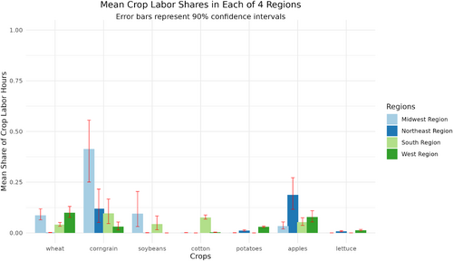
To examine regional variation in county crop employment shares by crop type, we calculate county-specific crop labor requirements per acre for each crop type across 500 random draws from the log normal distribution of labor intensity for each crop. We take the mean share of crop hours for specified crops in each county within the four US regions (as defined by the Census Bureau: Northeast, Midwest, South, and West). Figure B2 presents the mean share of total crop labor hours in the county for each region with 90% confidence intervals. The figure shows some overlap in the confidence intervals across regions and illustrates regional variation in concentration of crops grown. For example, the Midwest Region has higher shares of corn and soybeans than the rest of the country; the Midwest and West have higher shares of wheat; the South has a higher share of cotton; and the Northeast and West have higher shares of apples.
We next calculate county crop employment exposure to import tariffs pre- and post-NAFTA from the 500 simulations with random draws of labor hours per acre for every crop and find the change in crop employment exposure to tariffs. Figure B3 shows county-level standard deviation in changes in crop labor exposure to tariffs pre- and post-NAFTA relative to the county-level mean of the change in tariff exposure (i.e., county level coefficients of variation). Relatively small coefficients of variation provide suggestive evidence that measurement error in crop hours per acre have little impact on our main results since the variation in crop labor exposure to tariffs is small relative to the mean for most counties.
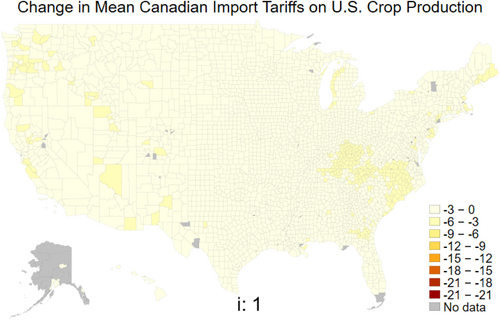
Finally, to confirm that the interpretation of our results does not change meaningfully across random draws of the labor intensity distributions, we created GIFs showing the maps generated from a random sample of 25 of the 500 Monte Carlo simulations. Figures B4-B7 show the GIFs for simulated variation in crop labor exposure to changes in tariffs imposed by Mexico and Canada on US crops and to changes in US tariffs on Mexico and Canada. Although small variations are observed in the GIF, the regions most exposed to tariff changes remain relatively consistent across Monte Carlo draws. Thus, our findings appear robust in the presence of random measurement error in crop labor intensity measures.
APPENDIX C: RURAL AND URBAN COUNTIES IN 1993
Figure C1 shows a map of counties by rural/urban classification, as classified in 1993, to illustrate the extent to which rural and urban counties were most exposed to tariff changes by sector during NAFTA. We use the Rural–Urban Continuum Code (RUCC) to define rural and urban areas, where nonmetro counties are categorized as rural and metro counties as urban.
APPENDIX D: LABOR EXPOSURE TO TARIFF CHANGES AS A SHARE OF TOTAL COUNTY EMPLOYMENT: CASE OF PROCESSED FOODS AND BEVERAGES
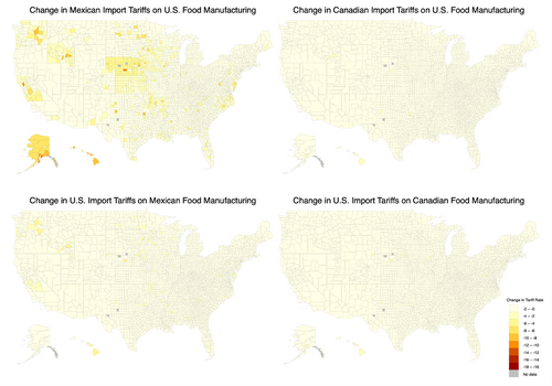
Since we include lightly processed foods and beverages in the crop and livestock sectors, one might be curious how much the tariffs in lightly processed agricultural goods contributes to changes in crop tariffs when weighted by their share in total county employment. We investigate this by creating a map, shown in Figure D1, of total employment exposure to tariff changes in food, beverage, and tobacco manufacturing. To calculate labor exposure for these sectors, we match industries defined by NAICS 311 and NAICS 312 to HS6-level tariffs, and we calculate labor exposure as we do for the non-agricultural sector, weighting by food manufacturing sector labor share of total employment in the county. The labor exposure to changes in tariff rates are generally small, and counties with high crop employment exposure generally have low food manufacturing exposure. This suggests that labor employed in lightly processed foods are not driving our findings related to crop labor shares of total county employment.10
APPENDIX E: CROP AND LIVESTOCK INDUSTRY LOCATIONS
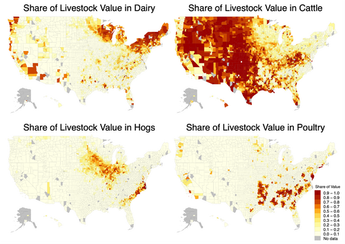
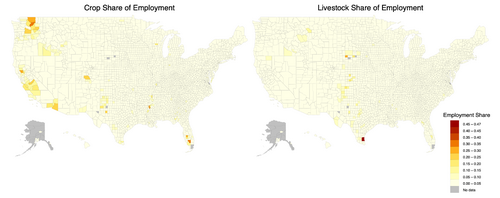
To better understand how geographic concentrations of employment in specific crops and livestock industries is related to labor exposure to tariff changes, we map shares of county crop and livestock employment by crop and livestock type.
Figure E1 maps county shares of crop employment for wheat, corn, soybeans, and cotton. Even though the United States is a major producer of these crops, these crops are highly mechanized and not labor-intensive. Nevertheless, in some counties, crop workers might be employed in only one or few crops. We find little labor exposure to changes in tariffs in the corn, soybean, and cotton producing counties during NAFTA because the tariff changes for these crops were much smaller than for some of the specialty fruit and vegetable crops. Wheat is grown in many rural counties, particularly along the Canadian border, and some of the wheat-producing counties appeared to have noticeable exposure to reductions in Mexican import tariffs on US crops during NAFTA.

Figure E2 maps county shares of crop employment for tobacco, vegetables,11 and fruit.12 These are more labor-intensive crops, and we see that counties with large shares of crop employment in tobacco were highly exposed to decreases in Mexican import tariffs during NAFTA. Counties with high concentration of crop labor in fruits were also exposed to large decreases in Mexican tariffs on crop imports. Many of the vegetable-producing counties throughout the United States were exposed to decreases in US tariffs on Mexican crops, but, in general, few counties were exposed to large changes in US import tariffs on Mexican or Canadian crops.
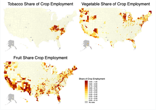
Figure E3 maps county shares of livestock employment for dairy, cattle, hogs, and poultry. Dairy producing counties were exposed to relatively large declines in US import tariffs during NAFTA, and hog-producing counties were exposed to relatively large declines in Mexican import tariffs.
Finally Figure E4 presents the county shares of employment for both crops and livestock.
Tariff changes for specific crops
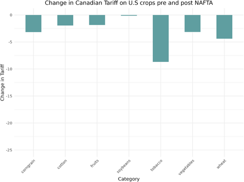
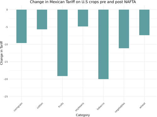
Since total crop employment in wheat, corn, soybeans, and cotton experienced relatively low exposure to tariff changes compared to fruits and vegetables, we examine the overall tariff changes to test if low tariff exposure in certain counties is due to concentration in crops with smaller tariff declines during NAFTA. We assess the average import tariff changes imposed on the United States across various crop categories, comparing at the mean tariff change for wheat, corn, soybeans, and cotton, as well as for fruits, vegetables, and tobacco.
We recalculate the base year import value-weighted tariffs () at the crop group level, , across key categories, including wheat, corn, soybeans, cotton, fruits, vegetables, and tobacco.
Figures E5 and E6 show the change and the percentage change in tariff between pre- and post-NAFTA period (2010). We see that overall, tobacco had the largest drop in tariffs for both Canada and Mexico. However, the change in Canadian import tariffs was much smaller in magnitude than the change in Mexican import tariffs. Mexican import tariffs on US fruits and vegetables were the next largest tariff changes following tobacco. Changes in Mexican import tariffs on US corn, wheat, cotton, and soybeans were relatively small.
