Robot Localization: An Introduction

Robot localization is the process of determining where a mobile robot is located with respect to its environment. Localization is one of the most fundamental competencies required by an autonomous robot as the knowledge of the robot's own location is an essential precursor to making decisions about future actions. In a typical robot localization scenario, a map of the environment is available and the robot is equipped with sensors that observe the environment as well as monitor its own motion. The localization problem then becomes one of estimating the robot position and orientation within the map using information gathered from these sensors. Robot localization techniques need to be able to deal with noisy observations and generate not only an estimate of the robot location but also a measure of the uncertainty of the location estimate. This article provides an introduction to estimation of theoretic solutions to the robot localization problem. It begins by discussing the mathematical models used to describe the robot motion and observations from the sensors. Two of the most common probabilistic techniques, the extended Kalman filter and the particle filter, that can be used to combine information from sensors to compute an estimate of the robot location are then discussed in detail and illustrated by simple examples. A brief summary of the large body of literature on robot localization is presented next. Appendices that present the essential mathematical background and alternative techniques are provided. The MATLAB code of the localization algorithms is also available.

1 Introduction

Robot localization provides an answer to the question: Where is the robot now? A reliable solution to this question is required for performing useful tasks, as the knowledge of current location is essential for deciding what to do next (1, 2). This article focuses on the solutions to the robot localization problem when the map of its environment is available. The problem then becomes one of estimating the robot pose (position and orientation) relative to the coordinate frame in which the map is defined. Typically, the information available for computing the robot location is gathered using onboard sensors, while the robot uses these sensors to observe its environment and its own motion. Given the space limitations, alternative scenarios where sensors such as surveillance cameras are placed in the environment to observe the robot or the robot is equipped with a receiver that provides an estimate of its location based on information from an external source (e.g., a Global Positioning System (GPS) that uses satellites orbiting the earth) are excluded from the following discussion.

A mobile robot equipped with sensors to monitor its own motion (e.g., wheel encoders and inertial sensors) can compute an estimate of its location relative to where it started if a mathematical model of the motion is available. This is known as odometry or dead reckoning. The errors present in the sensor measurements and the motion model make robot location estimates obtained from dead reckoning more and more unreliable as the robot navigates in its environment. Errors in dead reckoning estimates can be corrected when the robot can observe its environment using sensors and is able to correlate the information gathered by these sensors with the information contained in a map. How this can be achieved within a probabilistic framework will be discussed in this article.

The formulation of the robot localization problem depends on the type of the map available as well as on the characteristics of the sensors used to observe its environment. In one possible formulation, the map contains locations of some prominent landmarks or features present in the environment and the robot is able to measure the range and/or bearing to these features relative to the robot. Alternatively, the map could be in the form of an occupancy grid that provides the occupied and free regions of an environment and the sensors on board the robot measures the distance to the nearest occupied region in a given direction. As the information from sensors is usually corrupted by noise, it is necessary to estimate not only the robot location but also the measure of the uncertainty associated with the location estimate. Knowledge of the reliability of the location estimate plays an important role in the decision-making processes used in mobile robots as catastrophic consequences may follow if decisions are made assuming that the location estimates are perfect when they are uncertain. Bayesian filtering (3) is a powerful technique that could be applied to obtain an estimate of the robot location and the associated uncertainty. Both extended Kalman filter (EKF) and particle filter provide tractable approximations to Bayesian filtering and they are the focus of this article.

The remainder of this article is structured as follows. Section 2 provides the mathematical models for describing the robot motion and the relationships between the sensor measurements and the robot location for both feature-based and occupancy grip-based maps. Section 2.3 presents an algorithm based on the EKF for robot localization using a feature map. Section 1 presents a particle filter for locating a robot in a grid map. Section 2 presents a brief discussion of alternative localization techniques that have been proposed in the robotics literature. The mathematical background to estimation theory and two alternative robot localization techniques are presented in the appendices. The MATLAB code of the localization algorithms for the simple examples is available at https://github.com/UTS-CAS/Robot-Localization-examples and can also be downloaded here.

[ Download File ]

2 Vehicle Model and Sensor Models

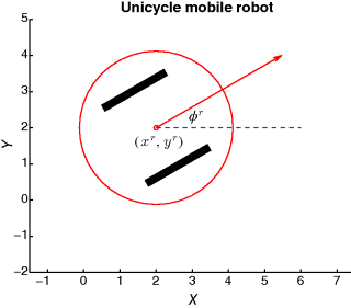
The mathematical ∼ models describing the behavior of the robot and the sensors mounted on it are the most important components in the formulation of the robot localization problem. The vehicle kinematic model describes the equations governing the robot motion in response to control actions. Figure 1 illustrates a differential drive robot operating on a two-dimensional plane where the forward velocity and the angular velocity of the robot body can be controlled using two motors that drive the two wheels. The differential equation that describes how the robot position and orientation evolve with time as a function of its forward and angular velocity is known as the robot motion model.

Details are in the caption following the image — **Figure 1**
Open in figure viewer PowerPoint

A differential drive robot operating in a two dimensional plane.

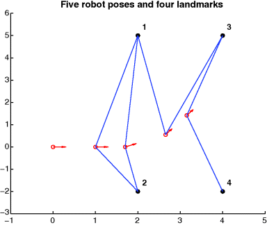
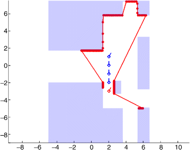
The relationship between the observations from the sensors and the location of the robot in the map is known as the sensor model. The sensor model is dependent on the characteristics of the sensor mounted on the robot as well as on the way the map of the environment is represented. As discussed in Section 1, the map of the environment is typically defined either using coordinates of known landmarks or features, or in the form of an occupancy grid where the status of each grid cell defines whether the area represented by the cell is occupied or free space. Figure 2 illustrates a map with four landmarks, while Figure 3 shows an occupancy grid map where the occupied areas are shaded.

In the following sections, a vehicle model and the sensor models typically used for robot localization are described. For simplicity and clarity of notation, it is assumed that the robot has three degrees of freedom and is moving in a two-dimensional plane.

2.1 Vehicle Model

The kinematic equations governing the motion of the differential drive robot illustrated in Figure 1 are given by

\begin{array}{l} {\overset{\cdot}{x}}^{r} (t) & = & (v (t) + δ v (t)) \cos (φ^{r} (t)) \\ {\overset{\cdot}{y}}^{r} (t) & = & (v (t) + δ v (t)) \sin (φ^{r} (t)) \\ {\overset{\cdot}{φ}}^{r} (t) & = & ω (t) + δ ω (t) \end{array}

(1)

where the coordinates x^r(t) and y^r(t) describe the position of the center of the mobile robot at time t, the orientation φ^r(t) is the angle between the heading of the robot and the x-axis of the fixed global coordinate frame.

{\dot{x}}^{r} (t)

denotes the derivative of x^r(t) with respect to time t. The forward velocity

v (t)

and angular velocity ω(t) are the control inputs of the robot.

δ v (t)

and δω(t) are the differences between the intended control value and the actual control values (control noises) and are assumed to be zero-mean Gaussian.

Discretizing the continuous-time motion model equation 1 with a sampling time ΔT and the Euler method results in

\begin{array}{l} x_{k + 1}^{r} & = & x_{k}^{r} + (v_{k} + δ v_{k}) Δ T \cos (φ_{k}^{r}) \\ y_{k + 1}^{r} & = & y_{k}^{r} + (v_{k} + δ v_{k}) Δ T \sin (φ_{k}^{r}) \\ φ_{k + 1}^{r} & = & φ_{k}^{r} + (ω_{k} + δ ω_{k}) Δ T \end{array}

(2)

where

(x_{k}^{r}, y_{k}^{r}, φ_{k}^{r})

is the robot location at time step k,

v_{k}

is the velocity at time k, and ω_k is the angular velocity at time k, and

δ v_{k}

and δω_k are the discrete time velocity noises and angular velocity noises, respectively.

2.2 Sensor Model for Landmark-Based Maps

Consider an environment that contains N₀ landmarks at known positions

(x_{L}^{i}, y_{L}^{i}), i = 1, \dots, N_{0}

. For simplicity, the uncertainties associated with landmark locations are assumed to be zero, although it is relatively straightforward to extend the analysis if this is not the case. At each time step while it is in motion, the robot observes the range (distance) and/or the bearing (relative angle) to one or more landmarks. Observation model provides a mechanism for computing the expected values of observations from sensors, given the knowledge of the map and an estimate of the robot location. If the sensor mounted on the robot observes both the range and the bearing to landmark i at time step k + 1, then the observation model is given by

\begin{array}{l} r_{k + 1}^{i} & = & \sqrt{{(x_{L}^{i} - x_{k + 1}^{r})}^{2} + {(y_{L}^{i} - y_{k + 1}^{r})}^{2}} + w_{r} \\ θ_{k + 1}^{i} & = & a \tan (\frac{y_{L}^{i} - y_{k + 1}^{r}}{x_{L}^{i} - x_{k + 1}^{r}}) - φ_{k + 1}^{r} + w_{θ} \end{array}

(3)

where

w_{r}

and

w_{θ}

are zero-mean Gaussian observation noises.

Laser range finders and ultrasonic sensors are most common sensors used for obtaining range and bearing measurements to landmarks. In case of a sensor that is only able to observe the bearing, for example, a camera, the equation for $θ_{k + 1}^{i}$ becomes the sensor model. A simple robot localization problem with a landmark-based map is illustrated in Figure 2.

2.3 Sensor Model for Occupancy Grid Maps

Occupancy grid maps provide a discretized representation of an environment where each of the grid cells is classified into two categories: occupied or free. Consider the scenario where a sensor on the robot can determine the distance to the nearest occupied grid cell along a given direction. A laser range finder is such a sensor. These sensors consist of a laser beam that rotates at a relatively high speed on the order of tens of revolutions per second and measures the distance to the obstacle that reflects it. If there is no obstacle within the sensor range, a reflection is not received and the sensor typically reports a nominal maximum distance d_max. Although the range measurements obtained depend on the environment and the robot location, it is not feasible to find an analytical observation model of the form equation 3 in this scenario. However, given an estimate of the robot location and the grid map, the expected value of a range measurement can be numerically obtained using ray casting (4). This makes it possible to evaluate the likelihood of a given pose, which is sufficient in some localization approaches such as a particle filter (see Section 4 for details).

Figure 3 shows a simple example of a robot localization problem where a laser range finder observes an environment described using an occupancy grid. The robot moves a few steps in the environment. The scan provided by the sensor at the first pose is shown in red.

3 Extended Kalman Filter for Localization in Landmark-Based Maps

The localization problem in a landmark-based map is to find the robot pose at time k + 1 as

x_{k + 1} = {(x_{k + 1}^{r}, y_{k + 1}^{r}, φ_{k + 1}^{r})}^{T}

(4)

given the map, the sequence of robot actions

v_{i}, ω_{i} (i = 0, \dots, k)

, and sensor observations from time 1 to time k + 1.

In its most fundamental form, the problem is to estimate the robot poses x_i (i = 0, …, k + 1) that best agree with all robot actions and all sensor observations. This can be formulated as a nonlinear least-squares problem using the motion and observation models derived in Section 2. The solution to the resulting optimization problem can then be calculated using an iterative scheme such as Gauss–Newton to obtain the robot trajectory and as a consequence the current robot pose. Appendix Appendix and Appendix Appendix provide the details on how both linear and nonlinear least-squares problems can be solved, and how the localization problem can be formulated as a nonlinear least-squares problem. The dimensionality of the problem is 3(k + 1) for two-dimensional motion, and given the sampling rate of modern sensors are on the order of tens of hertz, this strategy quickly becomes computationally intractable.

If the noises associated with the sensor measurements can be approximated using Gaussian distributions, and an initial estimate for the robot location at time 0, described using a Gaussian distribution x₀ ∼ $N ({\hat{x}}_{0}, P_{0})$ with known ${\hat{x}}_{0}, P_{0}$ is available (in this article, $\hat{x}$ is used to denote the estimated value of x), an approximate solution to this nonlinear least-squares problem can be obtained using an EKF. EKF effectively summarizes all the measurements obtained in the past in the estimate of the current robot location and its covariance matrix. When a new observation from the sensor becomes available, the current robot location estimate and its covariance are updated to reflect the new information gathered. Essential steps of the EKF-based localization algorithm are described in the following:

Let us denote

u_{k} = {(v_{k}, ω_{k})}^{T}, w_{k} = {(δ v, δ ω)}^{T} .

(5)

Then the nonlinear process model (from time k to time k + 1) as stated in equation 2 can be written in a compact form as

x_{k + 1} = f (x_{k}, u_{k}, w_{k})

(6)

where f is the system transition function, u_k is the control, and w_k is the zero-mean Gaussian process noise w_k ∼ N(0, Q).

Consider the general case where more than one landmark is observed. Representing all the observations

r_{k + 1}^{i}, θ_{k + 1}^{i}

together as a single vector z_k+1, and all the noises

w_{r}, w_{θ}

together as a single vector v_k+1, the observation model at time k + 1 as stated in equation 3 can also be written in a compact form as

z_{k + 1} = h (x_{k + 1}) + v_{k + 1}

(7)

where h is the observation function obtained from equation 3 and v_k+1 is the zero-mean Gaussian observation noise v_k+1 ∼ N(0, R).

Let the best estimate of x_k at time k be

x_{k} \sim N ({\hat{x}}_{k}, P_{k}) .

(8)

Then the localization problem becomes one of estimating x_k+1 at time k + 1:

x_{k + 1} \sim N ({\hat{x}}_{k + 1}, P_{k + 1})

(9)

where

{\hat{x}}_{k + 1}, P_{k + 1}

are updated using the information gathered using the sensors. EKF framework achieves this as follows. To maintain clarity, only the basic equations are presented in the following, while Appendix Appendix provides a more detailed explanation.

Predict using process model:

{\overline{x}}_{k + 1} = f ({\hat{x}}_{k}, u_{k}, 0)

(10)

\begin{matrix} {\overline{P}}_{k + 1} & = & J_{f_{x}} ({\hat{x}}_{k}, u_{k}, 0) P_{k} J_{f_{x}}^{T} ({\hat{x}}_{k}, u_{k}, 0) \\ + J_{f_{w}} ({\hat{x}}_{k}, u_{k}, 0) {QJ}_{f_{w}}^{T} ({\hat{x}}_{k}, u_{k}, 0) \end{matrix}

(11)

where

J_{f_{x}} ({\hat{x}}_{k}, u_{k}, 0)

is the Jacobian of function f with respect to x,

J_{f_{w}} ({\hat{x}}_{k}, u_{k}, 0)

is the Jacobian of function f with respect to w, both evaluated at

({\hat{x}}_{k}, u_{k}, 0)

Update using observation:

{\hat{x}}_{k + 1} = {\overline{x}}_{k + 1} + K (z_{k + 1} - h ({\overline{x}}_{k + 1}))

(12)

P_{k + 1} = {\overline{P}}_{k + 1} - {KSK}^{T}

(13)

where the innovation covariance S (here

z_{k + 1} - h ({\overline{x}}_{k + 1})

is called innovation) and the Kalman gain K are given by

S = J_{h} ({\overline{x}}_{k + 1}) {\overline{P}}_{k + 1} J_{h}^{T} ({\overline{x}}_{k + 1}) + R

(14)

K = {\overline{P}}_{k + 1} J_{h}^{T} ({\overline{x}}_{k + 1}) S^{- 1}

(15)

where

J_{h} ({\overline{x}}_{k + 1})

is the Jacobian of function h with respect to x evaluated at

{\overline{x}}_{k + 1}

Recursive application of the above equations every instant a new observation is gathered yields an updated estimate for the current robot location and its uncertainty. This recursive nature makes EKF the most computationally efficient algorithm available for robot localization.

An important prerequisite for EKF-based localization is the ability to associate measurements obtained with specific landmarks present in the environment. Landmarks may be artificial, for example, laser reflectors, or natural geometric features present in the environment such as line segments, corners, or planes (5, 6). In many cases, the observation itself does not contain any information as to which particular landmark is being observed. Data association is the process in which a decision is made as to the correspondence between an observation from the sensor and a particular landmark. Data association is critical to the operation of an EKF-based localizer, as catastrophic failure may result if data association decisions are incorrect.

EKF relies on approximating the nonlinear motion and observation models using linear equations and that the sensor noises can be approximated using Gaussian distributions. These are reasonable assumptions under many practical conditions and therefore EKF is the obvious choice for solving the robot localization problem when the map of the environment consists of clearly identifiable landmarks.

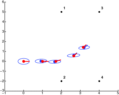
Figure 4 shows the result of EKF localization for the simple problem given in Figure 2. The ground truth of the robot poses and the estimated robot poses are shown in red and blue, respectively. The 95% confidence ellipses obtained from the covariance matrices in the EKF estimation process are also shown in the figure.

4 Particle Filter for Localization in Grid Maps

There are two important situations where EKF is not the method of choice for robot localization. The first is when the environment is represented by an occupancy grid. Sensor model for occupancy grid maps described in Section 2.3 is not an analytic model but based on the numerical process of ray casting and as such is unsuitable for use with an EKF. The other situation is when initial robot location is completely unknown, usually known as the global localization problem. In this case, the location of the robot needs to be described using an arbitrary probability distribution; thus, the Gaussian assumption that is the basis of the EKF formulation is violated. In general, manipulating arbitrary probability distributions is computationally intractable. One possible strategy is to discretize the space of possible robot locations and thus deal with manipulating discrete probability distribution. This method is known as Markov localization. The computation burden associated with Markov localization is proportional to the size of the environment and the resolution of the discretization, making this strategy unsuitable in many situations. Markov localization is described in Appendix Appendix .

In the particle filter localization (also known as Monte Carlo localization) (7), rather than discretizing the space of robot locations, a weighted set of robot location estimates, termed as particles, is used to describe the probability distribution of the robot location. As the computations are focused on particles and more particles are placed at more probable robot locations, the particle filters provide a more efficient alternative to Markov localization. Number of particles used determines the accuracy of the representation. However, increasing the number of particles to obtain a higher accuracy leads to a more costly estimation process.

In the particle filter, each particle in effect provides a guess as to the location of the robot. Thus, each particle is represented by three variables (x, y (position), φ (orientation)) for a robot operating in a two-dimensional plane. Each particle i has a weight $w_{i}$ that indicates the contribution of that particular particle to the probability distribution. The sum of the weights of all particles is set to 1, that is, $\sum_{i = 1}^{n} w_{i} = 1$ , where n is the total number of particles used. A collection of such guesses describes the best knowledge available, usually termed the belief, as to the true location of the robot. In the case of global localization, the initial robot location is completely unknown; therefore, all locations of the environment are equally likely to contain the robot. Thus, a set of equally weighted particles uniformly distributed in the environment is used to represent the belief of the robot location. During the localization process, this belief is updated as more and more information is acquired from the sensors.

In the particle filter, every time information from the sensors is gathered, the current belief is updated. The process is as follows (8, 9):

Prediction:When the robot is commanded to move, the new belief is obtained by moving each particle according to the motion model equation 2 with randomly generated $δ v_{k}, δ ω_{k}$ .
Update:When a new sensor observation is received, the belief is updated using an observation model. In this step, the weights of the particles are changed to reflect the likelihood that the true robot location coincides with the corresponding particle. In the case of j^th observation from a laser range finder, ray casting from each particle is used to obtain an expected measurement ${\hat{d}}_{j}$ . If the actual measurement is given by d_j and if the sensor noise is assumed to be zero mean with a variance $σ_{d}^{2}$ , the likelihood can be computed using a Gaussian distribution based on
$\frac{1}{σ_{d} \sqrt{2 π}} \exp {- \frac{{({\hat{d}}_{j} - d_{j})}^{2}}{2 σ_{d}^{2}}} .$ (16)
As at a given instance multiple independent range observations are acquired from the sensor, likelihood of obtaining a sequence of observations is computed by multiplying together all the likelihood. Once likelihoods of all the particles are computed, these are normalized to obtain the weight of each of the particles.
Resampling:This is performed to avoid the situation where a small number of particles with large weights dominate the representation of the belief. One common strategy used for resampling (10) is as follows:
1. Compute an estimate of the effective number of particles as
  $n_{eff} = \frac{1}{\sum_{i = 1}^{n} w_{i}^{2}} .$ (17)
2. If n_eff is less than a threshold, then draw n particles from the current particle set with probabilities proportional to their weights. Replace the current particle set with this new one. Set the weights of each particle to be 1/n.
Resulting set of particles represents the updated belief of the robot location.

This process is repeated as new control actions are taken and new observations become available. The mean or the mode of the corresponding probability distribution can be used if a numerical value for the best estimate of the robot location is desired.

Figure 5 shows the result of particle filter localization for the simple problem given in Figure 3. The particles, the best estimate of the robot location, and the ground truth robot location at the last step are shown in green, blue, and red, respectively.

5 Alternative Localization Techniques

When a map of the environment is not available, the robot localization problem becomes significantly more challenging. In this case, the problem becomes one of estimating both the robot location and landmark locations simultaneously. In the past 15 years, robust and efficient methods to dealing with robot localization in unknown environments, also known as the simultaneous localization and mapping (SLAM) problem (3), have emerged. SLAM in a feature-based environment has been well studied and it has been shown that both EKF and least-squares optimization could be used to reliably solve SLAM in most cases (11, 12). Presence of efficient solvers for very large-scale nonlinear least-squares optimization problems (13) has resulted in real-time solutions to the robot location estimation in unknown environments. Due to their low cost and presence of algorithms that extract rich information, cameras have become an important sensor in many robot navigation applications. A comprehensive survey on vision-based navigation is reported in Reference (14), while a recent strategy for SLAM using information from a camera is reported in Reference (15). Combining information from monocular cameras with inertial sensors makes it possible to obtain reliable localization in real time with a high level of accuracy (16).

An alternative method for localization in unknown environments is to simply use the information from a sensor such as a laser range finder to obtain the translation and rotation relating two robot poses from which two laser scans are taken. This is done through scan matching that aligns the two scans. Collection of such relative pose estimates can be used to formulate a nonlinear least-squares problem that can be solved to estimate all the robot poses (17). A modern solver such as g2o (13) could be used to efficiently obtain the location estimates. A representation of the environment (map) is not estimated. This strategy is called pose-graph SLAM (18). For a feature-based or pose-graph SLAM technique to be effective, a strategy to recognize the fact that the robot has returned to areas it has visited before, known as loop closure, is required. The reliable detection of loop closure is one of the remaining challenges for both feature-based SLAM and pose-graph SLAM (19).

Many other interesting robot localization problems and alternative solutions have been reported in the literature. Typical examples are localization using signal strengths from wireless infrastructure (20) and RFIDs (21), fusion of information from GPS and inertial navigation units (22), and an optimization technique for localization in grid maps (23) based on chamfer distance (24) that does not rely on many tuning parameters as is usually the case with particle filters.

The problem of estimating robot location given a map is now considered a solved problem, although highly dynamic environments populated with people pose significant challenges in practical deployments. The more complex problem of continuously estimating robot location within an unknown environment over a long period is still the subject of much research.

Appendix A: Least Squares Problem and Gauss–Newton Iteration

1 Linear Least Squares Problem and Solution

A linear least squares problem is to find X that minimizes

\begin{matrix} {| | b - A X | |}^{2} \overset{Δ}{=} = {(b - A X)}^{T} (b - A X) \end{matrix}

for given b, A, where

\begin{matrix} b = [\begin{matrix} \begin{matrix} b_{1} \\ b_{2} \\ ⋮ \\ b_{m} \end{matrix} \end{matrix}], {X \end{matrix} = [\begin{matrix} \begin{matrix} x_{1} \\ x_{2} \\ ⋮ \\ x_{n} \end{matrix} \end{matrix}], m \geq n

and

\begin{matrix} A = [\begin{matrix} \begin{matrix} a_{11} & a_{12} & \dots & a_{1 n} \\ a_{21} & a_{22} & \dots & a_{2 n} \\ ⋮ & ⋮ & ⋮ & ⋮ \\ a_{m 1} & a_{m 2} & \dots & a_{mn} \end{matrix} \end{matrix}] . \end{matrix}

Assuming that the matrix A is full column rank, the above problem has a closed-form solution:

X X^{*} = {(A^{T} A)}^{- 1} A^{T} b .

(18)

This can be obtained by expanding the objective function

\begin{array}{l} \begin{array}{l} E (X) & = & | | b - A X | |^{2} = {(b - A X)}^{T} (b - A X) \\ = & b^{T} b - 2 b^{T} A X + X^{T} A^{T} A X \end{array} \end{array}

and finding stationary points by letting

\begin{array}{l} \frac{d E}{d X} = 2 A^{T} A X - 2 A^{T} b = 0 \end{array}

which leads to the solution equation 18.

2 Weighted Linear Least Squares Problem and Solution

A weighted linear least squares problem is to find X that minimizes

\begin{array}{l} {(b - A X)}^{T} P^{- 1} (b - A X) \end{array}

where P is a positive definite matrix.

The closed-form solution to the weighted linear least-squares problem is

X^{*} = {(A^{T} P^{- 1} A)}^{- 1} A^{T} P^{- 1} b .

(19)

3 Nonlinear Least Squares and Gauss–Newton Iteration

A nonlinear least squares problem is to find X that minimizes

\begin{array}{l} {| | Z - F (X) | |}^{2} = {[Z - F (X)]}^{T} [Z - F (X)] \end{array}

where Z = [z₁, z₂, …, z_m]^T, X = [x₁, x₂, …, x_n]^T,

\begin{array}{l} F (X) = [\begin{array}{l} \begin{array}{l} f_{1} (X) \\ f_{2} (X) \\ ⋮ \\ f_{m} (X) \end{array} \end{array}] = [\begin{array}{l} \begin{array}{l} f_{1} (x_{1}, x_{2}, \dots, x_{n}) \\ f_{2} (x_{1}, x_{2}, \dots, x_{n}) \\ ⋮ \\ f_{m} (x_{1}, x_{2}, \dots, x_{n}) \end{array} \end{array}] \end{array}

with m ≥ n.

In general, closed-form solution for a nonlinear least squares problem cannot be obtained. Many techniques for solving nonlinear least squares problems are based on iteration.

Suppose X is close to X₀, by linearization,

\begin{array}{l} F (X) \approx F (X_{0}) + J_{F} (X_{0}) (X - X_{0}) \end{array}

where JF(X₀) is the Jacobian matrix given by

J_{F} (X) = [\begin{array}{l} \frac{\partial f_{1}}{\partial x_{1}} & \frac{\partial f_{1}}{\partial x_{2}} & \dots & \frac{\partial f_{1}}{\partial x_{n}} \\ \frac{\partial f_{2}}{\partial x_{1}} & \frac{\partial f_{2}}{\partial x_{2}} & \dots & \frac{\partial f_{2}}{\partial x_{n}} \\ : & : & : & : \\ \frac{\partial f_{m}}{\partial x_{1}} & \frac{\partial f_{m}}{\partial x_{2}} & \dots & \frac{\partial f_{m}}{\partial x_{n}} \end{array}]

evaluated at X₀.

Thus,

\begin{array}{l} Z - F (X) \approx Z - F (X_{0}) + J_{F} (X_{0}) X_{0} - J_{F} (X_{0}) X . \end{array}

Let

\begin{array}{l} A = J_{F} (X_{0}), b = Z - F (X_{0}) + J_{F} (X_{0}) X_{0} . \end{array}

Assuming that the matrix J_F(X₀) is full column rank, using the linear least square solution equation 18, we get

\begin{array}{l} X_{1} & = & {[J_{F}^{T} (X_{0}) J_{F} (X_{0})]}^{- 1} J_{F}^{T} (X_{0}) \\ [Z - F (X_{0}) + J_{F} (X_{0}) X_{0}] . \end{array}

(20)

In general, the iteration step is

\begin{array}{l} X_{k + 1} & = & {[J_{F}^{T} (X_{k}) J_{F} (X_{k})]}^{- 1} J_{F}^{T} (X_{k}) \\ [Z - F (X_{k}) + J_{F} (X_{k}) X_{k}] . \end{array}

(21)

Iterating until convergence leads to the optimum solution, provided that the initial guess X₀ is sufficiently close to the solution. This is known as the Gauss–Newton iteration.

4 Weighted Nonlinear Least Squares Problem

The weighted nonlinear least squares problem is to find X that minimize

{[Z - F (X)]}^{T} P^{- 1} [Z - F (X)]

(22)

where P is the covariance matrix of the noises contained in the measurement (data) Z.

Given the initial value X₀, Gauss–Newton iteration step is

\begin{array}{l} X_{k + 1} & = & {[J_{F}^{T} (X_{k}) P^{- 1} J_{F} (X_{k})]}^{- 1} \\ J_{F}^{T} (X_{k}) P^{- 1} [Z - F (X_{k}) + J_{F} (X_{k}) X_{k}] . \end{array}

(23)

Appendix B: Least Squares Method for Landmark Based Localization

Least squares method provides a way to optimally estimate the robot trajectory using all the available robot motion and observation information up to time k + 1. In least squares method, we estimate all the robot poses together instead of only the last pose as in the case of both the EKF and the particle filter based robot localization.

The state vector in least squares method is

X = {(x_{0}, x_{1}, \dots, x_{k}, x_{k + 1})}^{T} .

(24)

Note that the initial state mean value can be expressed as an observation of x₀:

{\hat{x}}_{0} = x_{0} + v_{x_{0}}

(25)

where

v_{x_{0}} \sim N (0, P_{0})

is the “observation noise”.

The motion model equation 2 can be rewritten as

\begin{array}{l} v_{k} & = & \frac{\sqrt{{(x_{k + 1}^{r} - x_{k}^{r})}^{2} + {(y_{k + 1}^{r} - y_{k}^{r})}^{2}}}{Δ T} - δ v_{k} \\ ω_{k} & = & \frac{φ_{k + 1}^{r} - φ_{k}^{r}}{Δ T} - δ ω_{k} . \end{array}

(26)

Now all the information available from time 0 to time k + 1 is summarized in

\begin{array}{l} Z & = & ({\overset{\land}{x}}_{0}^{T}, v_{0}, w_{0}, \dots, r_{1}^{i}, θ_{1}^{i}, \dots, \\ v_{k}, w_{k}, \dots, r_{k + 1}^{i}, θ_{k + 1}^{i} {, \dots)}^{T} . \end{array}

(27)

The relation between Z and X is given by

Z = F (X) + V

(28)

where F(X) is the nonlinear function combining equations 3-25, and 26. V ∼ N(0, P) is the vector of all the noises where P is constructed by P₀, Q, R.

Now the localization problem can be formulated as a nonlinear least squares problem as in equation 22 and could be solved using Gauss–Newton iteration by equation 23.

Appendix C: Intuitive Explanations of the Kalman Filter

1 Kalman Filter Equations

When both the process model and the observation model are linear, they can be expressed by

x_{k + 1} = F x_{k} + G u_{k} + w_{k}

(29)

and

z_{k + 1} = H x_{k + 1} + v_{k + 1}

(30)

where x_k, x_k+1 are the system state at time k, k + 1, F is the system transition matrix, G is the gain of control u_k, and w_k is the zero-mean Gaussian process noise w_k ∼ N(0, Q), H is the observation matrix, and v_k+1 is the zero-mean Gaussian observation noise v_k+1 ∼ N(0, R).

In this case, the state estimation can be obtained using the following Kalman filter equations assuming the initial state x₀ follows a known Gaussian distribution $x_{0} \sim N ({\hat{x}}_{0}, P_{0})$ .

Predict using process model:

{\overline{x}}_{k + 1} = F {\hat{x}}_{k} + G u_{k}

(31)

{\overline{P}}_{k + 1} = {FP}_{k} F^{T} + Q

(32)

where

{\overline{x}}_{k + 1}

is the state estimate at time k + 1 before using the observation information at time k + 1, and

{\overline{P}}_{k + 1}

is its corresponding covariance matrix.

Update using observation:

{\hat{x}}_{k + 1} = {\overline{x}}_{k + 1} + K (z_{k + 1} - H {\overline{x}}_{k + 1})

(33)

P_{k + 1} = {\overline{P}}_{k + 1} - {KSK}^{T}

(34)

where the innovation covariance S (here

z_{k + 1} - H {\overline{x}}_{k + 1}

is called innovation) and the Kalman gain K are given by

S = H {\overline{P}}_{k + 1} H^{T} + R

(35)

K = {\overline{P}}_{k + 1} H^{T} S^{- 1} .

(36)

In the following, we will provide some intuitive explanations of the Kalman filter equations for the one-dimensional case.

2 One-Dimensional Gaussian Distribution and Its Information

If a random variable x follows a Gaussian distribution, it is denoted as

x ~ N (m, σ^{2})

(37)

where m is the mean and σ² is the variance.

(Fisher) information of a Gaussian distribution N(m, σ²) is the inverse of the variance,

I = \frac{1}{σ^{2}} .

(38)

Intuitively speaking, the larger the uncertainty, the smaller the information.

3 Important Properties of 1D Gaussian Distributions

The following are a few properties of 1D Gaussian distributions that are useful in deriving the Kalman filter equations:

For any constant a,
$x ~ N (m, σ^{2}) \Rightarrow a x ~ N (a m, a^{2} σ^{2}) .$ (39)
For any constant u,
$x ~ N (m, σ^{2}) \Rightarrow x + u ~ N (m + u, σ^{2}) .$ (40)
For two independent random variables x and y,
$\begin{array}{l} x ~ N (m_{x}, σ_{x}^{2}), y ~ N (m_{y}, σ_{y}^{2}) \\ \Rightarrow & x + y ~ N (m_{x} + m_{y}, σ_{x}^{2} + σ_{y}^{2}) . \end{array}$ (41)

4 One-Dimensional Kalman Filter Prediction

This section shows that the Kalman filter prediction equation can be obtained easily from the properties of 1D Gaussian distributions listed in Section 3.

Suppose the process model is

x_{k + 1} = x_{k} + u_{k} + w_{k}

(42)

where u_k is the control and

w_{k}

is the zero-mean Gaussian process noise with variance

σ_{u}^{2}

. That is,

w_{k} \sim N (0, σ_{u}^{2})

. It is also assumed that

w_{k}

is independent of x_k.

At time k, the estimate of x_k follows a Gaussian distribution

x_{k} \sim N ({\hat{x}}_{k}, σ_{k}^{2})

(see equation 8), thus, by equation 40,

x_{k} + u_{k} ~ N ({\overset{\land}{x}}_{k} + u_{k}, σ_{k}^{2}) .

(43)

Further by equation 41,

x_{k + 1} = (x_{k} + u_{k}) + w_{k} ~ N ({\overset{\land}{x}}_{k} + u_{k}, σ_{k}^{2} + σ_{u}^{2}) .

(44)

Thus, if we denote the estimate of x_k+1 (after the process but before the observation) as

x_{k + 1} ~ N ({\overline{x}}_{k + 1}, {\overline{σ}}_{k + 1}^{2})

(45)

then the prediction equations are

\begin{array}{l} {\overline{x}}_{k + 1} & = & {\overset{\land}{x}}_{k} + u_{k} \\ {\overline{σ}}_{k + 1}^{2} & = & σ_{k}^{2} + σ_{u}^{2} . \end{array}

(46)

Similarly, if the process model is

x_{k + 1} = {a x}_{k} + {b u}_{k} + w_{k}

(47)

where a, b are constants and

w_{k} \sim N (0, σ_{u}^{2})

, then the prediction equations become

\begin{array}{l} {\overline{x}}_{k + 1} & = & a {\overset{\land}{x}}_{k} + {b u}_{k} \\ {\overline{σ}}_{k + 1}^{2} & = & a^{2} σ_{k}^{2} + σ_{u}^{2} \end{array}

(48)

which are equations 31 and 32 when all variables are scalars.

5 One-Dimensional Kalman Filter Update

Suppose the observation model is

z_{k + 1} = x_{k + 1} + v_{k + 1}

(49)

where z_k+1 is the observation value at time k + 1 and

v_{k + 1}

is the zero-mean Gaussian observation noise with variance

σ_{z}^{2}

. That is,

v_{k + 1} \sim N (0, σ_{z}^{2})

. It is also assumed that

v_{k + 1}

is independent of x_k+1. By equation 39 (choosing a = − 1),

- v_{k + 1} ~ N (0, σ_{z}^{2}) .

(50)

By the observation model equation 49,

x_{k + 1} = - v_{k + 1} + z_{k + 1} .

(51)

Thus, by equation 40,

x_{k + 1} ~ N (z_{k + 1}, σ_{z}^{2}) .

(52)

The prior information about x_k+1 is given by equation 45 (after the prediction but before the update). So we have two pieces of information about x_k+1: one from observation equation 52 and one from prior equation 45.

According to the definition of information contained in a Gaussian distribution (see equation 38), the information (about x_k+1) contained in equation 45 is

I_{prior} = \frac{1}{{\overline{σ}}_{k + 1}^{2}}

(53)

while the information (about x_k+1) contained in equation 52 is

I_{obs} = \frac{1}{σ_{z}^{2}} .

(54)

The total information (about x_k+1) after the observation should be the sum of the two, namely,

I_{total} = I_{prior} + I_{obs} = \frac{1}{{\overline{σ}}_{k + 1}^{2}} + \frac{1}{σ_{z}^{2}} .

(55)

The new mean value is the weighted sum of the mean values of the two Gaussian distributions equations 45 and 52. The weights are decided by the proportion of information contained in each of the Gaussian distributions (as compared with the total information). That is,

\begin{array}{l} {\overset{\land}{x}}_{k + 1} & = & \frac{I_{prior}}{I_{total}} {\overline{x}}_{k + 1} + \frac{I_{obs}}{I_{total}} z_{k + 1} \\ = & \frac{σ_{z}^{2}}{{\overline{σ}}_{k + 1}^{2} + σ_{z}^{2}} {\overline{x}}_{k + 1} + \frac{{\overline{σ}}_{k + 1}^{2}}{{\overline{σ}}_{k + 1}^{2} + σ_{z}^{2}} z_{k + 1} . \end{array}

(56)

Note that the sum of the two weights is 1, that is, $\frac{I_{prior}}{I_{total}} + \frac{I_{obs}}{I_{total}} = 1$ .

The variance can be obtained by (see equation 38)

σ_{k + 1}^{2} = \frac{1}{I_{total}} = \frac{1}{1 / {\overline{σ}}_{k + 1}^{2} + 1 / σ_{z}^{2}} = \frac{{\overline{σ}}_{k + 1}^{2} σ_{z}^{2}}{{\overline{σ}}_{k + 1}^{2} + σ_{z}^{2}} .

(57)

So, the final estimate on x_k+1 (after the prediction and update) is

x_{k + 1} ~ N ({\overset{\land}{x}}_{k + 1}, σ_{k + 1}^{2})

(58)

where

{\hat{x}}_{k + 1}

and

σ_{k + 1}^{2}

are given in equations 56 and 57, respectively.

Figure 6 illustrates the update step of Kalman filter.

The update formulas, equations 56 and 57, can also be expressed as

\begin{array}{l} {\overset{\land}{x}}_{k + 1} & = & {\overline{x}}_{k + 1} + \frac{{\overline{σ}}_{k + 1}^{2}}{{\overline{σ}}_{k + 1}^{2} + σ_{z}^{2}} (z_{k + 1} - {\overline{x}}_{k + 1}) \\ σ_{k + 1}^{2} & = & {\overline{σ}}_{k + 1}^{2} (1 - \frac{{\overline{σ}}_{k + 1}^{2}}{{\overline{σ}}_{k + 1}^{2} + σ_{z}^{2}}) \\ = & {\overline{σ}}_{k + 1}^{2} - {\overline{σ}}_{k + 1}^{2} \frac{{\overline{σ}}_{k + 1}^{2}}{{\overline{σ}}_{k + 1}^{2} + σ_{z}^{2}} \\ = & {\overline{σ}}_{k + 1}^{2} - \frac{{\overline{σ}}_{k + 1}^{2}}{{\overline{σ}}_{k + 1}^{2} + σ_{z}^{2}} ({\overline{σ}}_{k + 1}^{2} + σ_{z}^{2}) \frac{{\overline{σ}}_{k + 1}^{2}}{{\overline{σ}}_{k + 1}^{2} + σ_{z}^{2}} . \end{array}

(59)

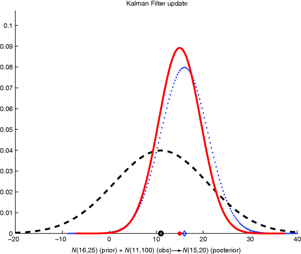
These are equations 33 and 34 (when all variables are scalars), where $z_{k + 1} - {\overline{x}}_{k + 1}$ is the innovation, ${\overline{σ}}_{k + 1}^{2} + σ_{z}^{2}$ is the innovation variance S, and $\frac{{\overline{σ}}_{k + 1}^{2}}{{\overline{σ}}_{k + 1}^{2} + σ_{z}^{2}}$ is the Kalman gain K.

Appendix D: Markov Localization

In Makov localization, rather than relying on a set of particles to represent a probability distribution, the state space is discretized into a grid and the probability that the robot is present in a particular grid cell is used to describe the estimate of the robot location. In a two-dimensional scenario, the discretization is over three–dimensional space incorporating the robot position and orientation.

At time k, the probability that the robot is present in each of the grid cells is represented by

p_{i} (k) \overset{Δ}{=} P (x_{k} = i), i = 1, \dots, M

(60)

where P(x_k = i) means the probability of robot pose x_k is in grid cell i, M is the total number of grid cells, and

\begin{array}{l} 0 \leq p_{i} (k) \leq 1, \sum_{i = 1}^{M} p_{i} (k) = 1 . \end{array}

This probability distribution is called belief bel(k).

Initial belief bel(0) is the prior distribution. When there is no prior knowledge about the robot location, the probability distribution is a uniform one. That is,

\begin{array}{l} p_{i} (0) = \frac{1}{M}, i = 1, \dots, M . \end{array}

Given a belief bel(k) at time k and a new control input u_k and a new observation z_k+1, the belief needs to be updated to find bel(k + 1) using Bayes filter. There are two essential steps used to update the belief:

Prediction:In this step the new control input u_k and the previous belief bel(k) are used to compute the predicted belief $\overline{bel (k + 1)}$ . Here $\overline{bel (k + 1)}$ is the prediction, which for any possible location j can be computed using
$\overline{p_{j} (k + 1)} = \sum_{i = 1}^{M} p_{i} (k) P (x_{k + 1} = j | x_{k} = i, u_{k}) . < / p > < / item 1 > < item 1 > < p >$ (61)
This equation is obtained using the law of total probabiliy. Here P(x_k+1 = j|x_k = i, u_k) is the conditional probability that can be obtained from the motion model.
Update:In this step, using Bayes' theorem, information in the new observation z_k+1 is fused with the prediction to obtain the new belief at time k + 1 as follows:
$\begin{array}{l} p_{j} (k + 1) & \overset{Δ}{=} & P (x_{k + 1} = j | z_{k + 1}) \\ = & \frac{P (z_{k + 1} | x_{k + 1} = j) \overset{̲}{p_{j} (k + 1)}}{\sum_{i = 1}^{M} P (z_{k + 1} | x_{k + 1} = i) \overset{̲}{p_{i} (k + 1)}} \end{array}$ (62)
where the conditional probability P(z_k+1|x_k+1 = i) can be obtained from the sensor model.

Bibliography

1 G. Georges, R. Sobek, and R. Chatila. A Multi-Level Planning and Navigation System for a Mobile Robot: A First Approach to Hilare. In Proc. 6th International Joint Conference on Artificial Intelligence; Vol. 1, Morgan Kaufmann Publishers Inc., 1979.
Google Scholar
2 H. F. Durrant-Whyte. Ind. Rob. 1994, 21, pp 11–16.
10.1108/EUM0000000004145
Web of Science® Google Scholar
3 S. Thrun, W. Burgard, and D. Fox. Probabilistic Robotics. MIT Press, 2005.
Google Scholar
4 H. Blume and B. Heimann. A Laser Range Scanner Simulation for Probabilistic Object Tracking, in ICRA 2007 Workshop: Planning, Perception and Navigation for Intelligent Vehicles; 2007.
Google Scholar
5 M. Drumheller. IEEE Trans. Pattern Anal. Mach. Intell. 1987, 2, pp 325–332.
10.1109/TPAMI.1987.4767907
Google Scholar
6 J. J. Leonard and H. F. Durrant-Whyte. IEEE Trans. Rob. Autom. 1991, 7, pp 376–382.
10.1109/70.88147
Web of Science® Google Scholar
7 I. M. Rekleitis. A Particle Filter Tutorial for Mobile Robot Localization. Centre for Intelligent Machines, Technical Report TR-CIM-04-02, 2004), McGill University.
Google Scholar
8 F. Dellaert, D. Fox, W. Burgard, and S. Thrun. Monte Carlo Localization for Mobile Robots. Proc. IEEE International Conference on Robotics and Automation; Vol. 2. IEEE, 1999.
Google Scholar
9 D. Fox, W. Burgard, F. Dellaert, and S. Thrun. Monte Carlo Localization: Efficient Position Estimation for Mobile Robots. Proc. Sixteenth National Conference on Artificial Intelligence; John Wiley & Sons Ltd, 1999.
Google Scholar
10 G. Kitagawa. J. Comput. Graph Stat. 1996, 5, pp 1–25.
10.2307/1390750
Google Scholar
11 G. Dissanayake, P. Newman, S. Clark, H. Durrant-Whyte, and M. Csorba. IEEE Trans. Rob. Autom. 2001, 17, pp 229–241.
10.1109/70.938381
Web of Science® Google Scholar
12 F. Dellaert and M. Kaess. Int. J. Rob. Res. 2006, 25(12), pp 1181–1203.
10.1177/0278364906072768
Web of Science® Google Scholar
13 R. Kummerle, G. Grisetti, H. Strasdat, K. Konolige, and W. Burgard. g2o: A General Framework for Graph Optimization. In Proc. IEEE International Conference on Robotics and Automation (ICRA); 2011, pp 3607–3613.
Google Scholar
14 G. N. DeSouza, and C. K. Avinash. Pattern Anal. Mach. Intell. 2002, 24, pp 237–267.
10.1109/34.982903
Web of Science® Google Scholar
15 L. Zhao, S. Huang, Y. Sun, L. Yan, and G. Dissanayake. Int. J. Rob. Res. 2015, 34(4-5), pp 493–516.
10.1177/0278364914551583
Web of Science® Google Scholar
16 J. Hesch, D. G. Kottas, S. L. Bowman, and S. Roumeliotis. IEEE Trans. Rob. 2014, 30, pp 158–176.
10.1109/TRO.2013.2277549
Web of Science® Google Scholar
17 F. Lu and E. Milios. Auton. Robots 1997, 4, pp 333–349.
10.1023/A:1008854305733
Web of Science® Google Scholar
18 G. Grisetti, R. Kmmerle, C. Stachniss, and W. Burgard. IEEE Intell. Trans. Syst. Mag. 2010, 2, pp 31–43.
10.1109/MITS.2010.939925
Web of Science® Google Scholar
19 Y. Latif, C. Cadena, and J. Neira. Int. J. Rob. Res. 2013, 32(14), pp 1611–1626.
10.1177/0278364913498910
Web of Science® Google Scholar
20 B. Ferris, D. Haehnel, and D. Fox. Gaussian Processes for Signal Strength-Based Location Estimation. In Proc. Robotics: Science and Systems; 2006.
Google Scholar
21 J. Zhou and J. Shi. J. Intell. Manuf. 2009, 20, pp 695–707.
10.1007/s10845-008-0158-5
Web of Science® Google Scholar
22 S. Sukkarieh, E. M. Nebot, and H. F. Durrant-Whyte. IEEE Trans. Rob. Autom. 1999, 15, pp 572–578.
10.1109/70.768189
Web of Science® Google Scholar
23 L. Dantanarayana, R. Ranasinghe, and G. Dissanayake. C-LOG: A Chamfer Distance Based Method for Localisation in Occupancy Grid-Maps. In 2013 IEEE/RSJ International Conference on Intelligent Robots and Systems (IROS), pp 376–381.
Google Scholar
24 G. Borgefors. Comput. Vis. Graph. Image Process. 1986, 34, pp 344–371.
10.1016/S0734-189X(86)80047-0
Web of Science® Google Scholar

Citing Literature

Wiley Encyclopedia of Electrical and Electronics Engineering

Browse other articles of this reference work: