Fast approximate 1D inversion of frequency domain electromagnetic data
ABSTRACT
We present a fast approximate method for 1D inversion of frequency domain data and apply it to frequency domain helicopter-borne data from the Bookpurnong area of the Murray River, South Australia. The method is based on fast approximate forward computation of transient electromagnetic step responses and their derivatives with respect to the model parameters of a 1D model, with the frequency domain responses and derivatives then found through Fourier transformation of the time-domain counterparts. The inversion is carried out with multi-layer models in an iterative, constrained least-squares inversion scheme including explicit formulation of the model regularization through a model covariance matrix. The method is 30 times faster than conventional full inversion for a layered earth model and produces model sections of concatenated 1D models and contoured maps of mean conductivity in elevation intervals almost indistinguishable from those of a conventional full inversion. In a theoretical forward and inverse modelling study, the fast approximate and conventional computation methods are compared demonstrating the applicability of the approximate method and its limitations.
Applied to the Bookpurnong RESOLVE® FDHEM data set from South Australia, the inversion produces model sections and conductivity maps that reveal the distribution of conductivity in the area and thereby the distribution of salinity. This information is crucial for any remediation effort aimed at alleviating the salinization of the river and the degradation of floodplain vegetation and associated ecosystems.
INTRODUCTION
Despite advances in computer speed and code efficiency, the method most often employed for the interpretation of frequency domain helicopter-borne electromagnetic (FDHEM) data is inversion with one-dimensional (1D) models. For large data sets, inversion with 2D and 3D models is not yet feasible because of the computational burden. Even with 1D models, inversion of huge data sets can still be computationally challenging, especially because new interpretation techniques involve the simultaneous inversion of many soundings with lateral constraints between the 1D models (Auken and Christiansen 2004; Brodie and Sambridge 2006) to ensure lateral continuity of the model sections of concatenated 1D models. The effect of 3D structures on 1D interpretation of transient electromagnetic (TEM) data have been dealt with in a number of papers, e.g., Auken (1995) and Hördt and Scholl (2004). In general, these studies show that, if the geological environment consists in slowly varying 3D structures with moderate resistivity contrasts, the 1D inversion approach is viable and will produce pseudo-2D images of concatenated 1D models that will be a good approximation to the real conductivity distribution, especially if lateral constraints are included in the inversion (Auken and Christiansen 2004; Brodie and Sambridge 2006; Christensen and Tølbøll 2009). In environments with pronounced 3D model characteristics, 1D inversion will in many cases provide unreliable models with artefacts know as ‘pant legs’. However, though it is not sufficient to prove that 3D effects are not present (Ellis 1998), none of these typical model artefacts have been seen in the inversion of the Bookpurnong FDHEM data.
For 1D inversion, more or less sophisticated approximate methods have been developed. These are often included in software packages used for data and model display and for the handling of limited geographical information (see, for example, EMflow (Macnae et al. 1998) and EMax (Fullagar and Reid 2001)). Successful fast approximate inversion techniques based on the general theoretical framework of approximate inverse mapping where a sufficiently accurate forward mapping is combined with approximate derivatives have been presented in Oldenburg and Ellis (1991) and Li and Oldenburg (1992).
A fairly comprehensive comparison between different inversion and transformation techniques used for FDHEM data was reported by Sattel (2005). In Table 1, the computation times are shown for a range of different techniques. Evidently, there is a huge difference between the conventional 1D inversion methods: Occam (Constable et al. 1987; Farquharson et al. 2003) and 3-and 4-layer inversion on the one side and the rapid imaging/ transformation methods: EMflow, differential resistivity (Huang and Fraser 1996) and the Sengpiel section method (Sengpiel 1988; Sengpiel and Siemon 2000) on the other. In terms of computation time, the Zohdy method presented by Sattel (2005) lies between these extremes.
| Algorithm | CPU time (s) |
|---|---|
| Zohdy | 80 |
| Occam | 6900 |
| 3-layer model | 240 |
| 4-layer model | 258 |
| EMflow | 30 |
| Differential resistivity | 1.9 |
| Sengpiel | 1.4 |
The method we shall present here falls in the same category as the Zohdy method as far as computation time is concerned. Using a similar number of layers as used in the Zohdy algorithm, the computation time of the approximate inversion technique of this paper would be  s for the profile used in Sattel (2005). Our approach is based on an approximate forward mapping combined with an iterative, constrained least squares inversion formulation and contrary to the Zohdy algorithm of Sattel (2005) the regularization of the inversion is explicitly and consistently formulated and posterior parameter uncertainties can be estimated.
The method of fast approximate inversion of FDHEM data presented here is based on the corresponding fast approximate inversion of TEM data (Christensen 2002; Christensen et al. 2009) and uses an approximate forward mapping together with an iterative, constrained least squares 1D inversion formulation. The approximate and conventional 1D inversion approaches share the inversion formulation, the difference lying only in the forward mapping.
Our method is verified through a theoretical modelling and inversion study comparing the performance of a conventional and approximate approach and by comparing the conventional forward responses of the models obtained in the approximate inversion with the data of the field example.
The approximate inversion method is applied to the FDHEM data set from Bookpurnong in the Murray River Basin, South Australia, recorded with the RESOLVE® system. The results are presented as model sections of concatenated 1D models and as contoured maps of mean conductivity in elevation and depth intervals. The fast approximate approach will be compared with conventional 1D inversion as well as imaging algorithms based on data transformation.
FAST APPROXIMATE INVERSION OF FDHEM DATA
The approximate forward mapping
In the papers by Christensen (2002) and Christensen et al. (2009) a fast approximate inversion method for transient electromagnetic data was presented. The method is general, supporting all configurations and field components, and it is approximately 50 times faster than conventional inversion. It is based on particular analytical properties of the transient step response that cannot be reproduced in the frequency domain and it therefore seems obvious to implement a fast approximate inversion method in the frequency domain by sine and cosine transformations of the time-domain responses and their derivatives with respect to the model parameters. By observing that  and
and  , the cosine and sine transforms are implemented using the fast Hankel transform filters of Christensen (1990).
 (1)
(1) (2)
(2) (3)
(3) (4)
(4) (5)
(5) (6)
(6) (7)
(7) is the horizontal distance between the transmitter and receiver coils. Scaling with the primary field and multiplying with 106 to get the relative amplitude in parts per million (ppm), we find for the inphase
  and quadrature
  parts
parts
 (8)
(8) (9)
(9)To be useful in an inversion scheme, not only the FDHEM forward responses need to be calculated but also their derivatives with regard to the model parameters. However, the time-domain approximate method also delivers the derivatives of the step response with regard to the model parameters,  . The derivatives with respect to the model parameters of the FDHEM response are calculated from their time-domain equivalents in a way similar to the response, using equations (8) and (9).
For all practical purposes, for the frequencies used in frequency domain EM methods, the time-domain step responses can be calculated sufficiently accurately at the early and late times necessary to give accurate high- and low-frequency domain responses, respectively. This is due to the fact that the time-domain step responses are found by interpolating in half-space responses and these are calculated through a fast Hankel transform of an analytical expression in the time/wavenumber domain; there is no transformation from frequency to time (or – equivalently – from Laplace domain to time).
Accuracy of the approximate FDHEM method
 (10)
(10)and the residuals are summed over all four test models. Essentially, all residuals are equal for sampling densities of 5 per decade or more, so we have chosen a density of 5 samples per decade in the following computations. For this choice, approximate and conventional responses for the four test models of Fig. 1 are shown in Fig. 2. A sampling density in time of 5 per decade, corresponds to 10 samples per decade in depth.
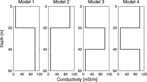
The conductivity as a function of depth for the four test models.
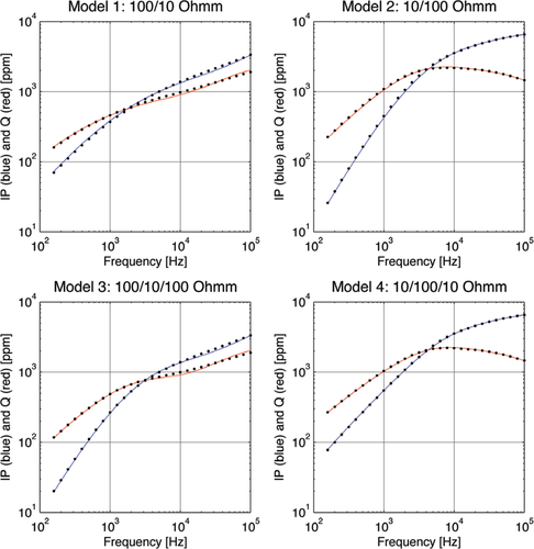
Conventional (full drawn curves) and fast approximate responses (dots) for the four models of Fig. 1.
To further illustrate the performance of the approximate inversion we have compared approximate forward responses and inversion results of theoretical data for 21 three-layer models with those of conventional calculations. For all 21 models, the resistivity of the first and third layers is  and the thicknesses of the first and second layer are 20 m. The resistivity of the second layer varies in ten steps both upwards and downwards with a factor of 1.4678 corresponding to a sampling density of 6 per decade in resistivity giving a total of 21 models. The resistivity of the second layer thus attains values from
  resulting in contrasts up to a factor of 50 with the surrounding layers. We have assumed a horizontal coplanar configuration with 8 m transmitter-receiver (Tx-Rx) separation, a survey height of 35 m and six frequencies: 0.1 kHz, 0.4 kHz, 1.6 kHz, 6.4 kHz, 25.6 kHz and 102.4 kHz.
 (11)
(11) (12)
(12)where  can be either the
  or
or  components and
  is the frequency. Figure 3 shows the maximum relative difference and residual. Obviously, the difference is the smallest for the smallest resistivity contrasts and increases for increasing contrast, however, most when the middle layer is more conductive. For all models, the normalized ed residual of
  is below 5% while the normalized residual for
  goes up to 8% for the lowest resistivity of the middle layer. The maximum relative difference stays below 5% for all contrasts when the second layer is resistive and below 10% for the conductive middle layer except for the first three models, i.e., when the contrast is below a factor of
  .
.
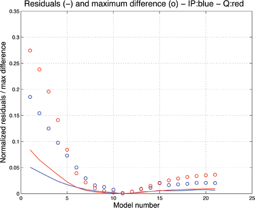
Normalized relative residual and maximum relative difference between the approximate and conventional responses of 21 three-layer models. Model 1 corresponds to the most conductive middle layer and model 21 to the most resistive.
To illustrate the inversion performance, we have used the conventional theoretical forward responses as data and ascribed noise (but not perturbed data) according to the noise model chosen for the survey data in Table 2. The theoretical data are then inverted with a 30-layer, multi-layer (smooth) model with both conventional computations and the fast approximate method.
| Frequency # | Frequency Hz | Configuration | PP noise (ppm) |
|---|---|---|---|
| 1 | 390 | HCP | 10 |
| 2 | 1,798 | HCP | 10 |
| 3 | 3,242 | VCX | 10 |
| 4 | 8,177 | HCP | 20 |
| 5 | 39,470 | HCP | 40 |
| 6 | 132,700 | HCP | 50 |
The results are seen in Fig. 4. The inverted models are very similar but the conventional inversion recovers the resistive middle layer slightly better than the approximate inversion. Both inversion methods have equal difficulties in delineating the bottom of the second layer when it is very conductive due to the limited depth penetration through the layer.
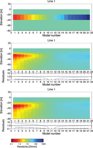
True models (top) and multi-layer inversion results of conventional inversion (middle) and approximate inversion (bottom). Model 1 corresponds to the most conductive middle layer and model 21 to the most resistive.
Another issue to consider is the configuration of the frequency domain system. For most of the configurations used in frequency domain methods, the corresponding time-domain step responses are quite slowly varying, especially for airborne methods and we believe that a sampling density of 5 per decade will generally be sufficiently accurate. In theory, for ground based frequency domain methods with large separations between transmitter and receiver, the corresponding time-domain step response may have an abrupt sign change at very early times, so in this situation, for very high frequencies in the frequency domain, a sampling density of 5 per decade may not suffice. However, ground-based frequency domain methods with large Tx-Rx separations and very high frequencies are not used because they are extremely unstable.
Inversion methodology
 iteration is given by
 (13)
(13)where  is the model vector containing the logarithm of the model parameters,
  is the Jacobian matrix containing the derivatives of the data with respect to the model parameters,
  is the vector transpose (and conjugate, if complex),
  is the data error covariance matrix,
  is the covariance matrix of the prior model,
  is a model covariance matrix imposing the vertical smoothness constraint of the multi-layer models,
  is the Marquard damping factor,
  is the identity matrix,
  is the field data vector,
  is the non-linear forward response vector of the
  model and
  is the prior model vector. In this study, as is most often the case, the data noise is assumed to be uncorrelated, implying that
  is a diagonal matrix.
 , given by
 (14)
(14)Where  is based on the final model. The analysis is expressed through the standard deviations of the model parameters obtained as the square root of the diagonal elements of
  (e.g., Inman et al. 1975).
The multi-layer model
The models used in the approximate inversion are multi-layer models, sometimes called ‘smooth’ models, where the subsurface is divided into a large number of layers. In the iterative inversion, the layer boundaries are kept fixed and only the layer resistivities are changed in the inversion. In this study we have used a 30 layer model where the depths to the layer boundaries increase as a hyperbolic sine of the layer number. In this way, the depths to the layer boundaries increase linearly for small depths so that the top layers are all of approximately the same thickness and the depths to the layer boundaries increase exponentially at large depths so that the thickness of a layer is a factor times the previous one.
In our 30-layer model, the top layer is 2 m thick and the deepest layer boundary is at a depth of 165 m. The asymptotic exponential factor is  , corresponding to about 24 layers per decade. The initial model is a homogeneous half-space with resistivity
  .
.
A proper multi-layer model must be an oversampling of the subsurface in relation to the information contents of the data, i.e., none of the layers must be individually resolved and the depth to the bottom layer boundary must be well below the penetration depth of the data. The initial model should have a resistivity that permits the sensitivity of the lowest frequencies to reach the bottom of the model. If the initial resistivity is too low, convergence will be slower because the first iterations will not contain information about the resistivity at the deeper parts of the model.
The model covariance matrix
 (15)
(15)where  is the von Karman covariance function of order
  and correlation length
  is the factor
  between the correlation lengths,
  is the number of stacked single-scale covariance functions and
  is the standard deviation of the correlation. In this study we have used
  ,
,  ,
,  and
and  . This means that the covariance function will contain correlation lengths between 6,500 km and 0.65 cm, one per decade. This covers scales of geological variability between the radius of the Earth and pebbles: clearly sufficient for airborne FDHEM data. Using the broadband covariance functions defined above ensures that the model structure at all scales will be permitted if required by the data. Notice that the model covariance matrix only depends on the geometry of the multi-layer model and so it needs to be calculated and inverted only once for the whole data inversion process. The broadband covariance function also has the desirable property that, for a given
  , the regularization level does not depend on model discretization.
 for the single-scale correlation function with correlation length
  , between the layers defined by the depth intervals of
  and
and  , is given by:
 (16)
(16) , the integration must be split into two intervals according to the sign of
 (17)
(17)Choosing the regularization level
It is crucial for the inversion to choose  correctly in relation to the model and the information content of the data. If chosen too small, the model will not show all the structure that can be resolved by the data and if chosen too large, the models will become erratic and the inversion will fit the data noise. The practical inversion is done on the logarithm of resistivities and the model covariance matrix thus relates to this parameter.
Experiments have been carried out for both the approximate inversion and the conventional inversion on data from Line 60010 of the RESOLVE® data set with values of  defined between 0.25–4.00 in steps of 0.25. In Fig. 5, selected model sections for a range of standard deviations are shown for the approximate inversion and a pragmatic inspection of the model sections reveals that a value of 2.0 seems to be appropriate. A similar result was obtained for the conventional inversion (not shown) and in the comparisons between fast approximate and conventional inversion in the following sections, the regularization level has been set to be the same for the two methods.
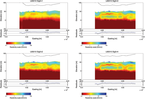
Model sections of concatenated 1D inverse models from line 60010, inverted with different values of the model covariance matrix standard deviation,  .
.
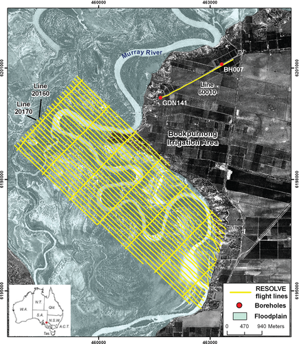
Location map of the Bookpurnong survey area showing the Bookpurnong floodplain and the adjacent highland. Aerial photo overlain with the RESOLVE® FDHEM survey lines.
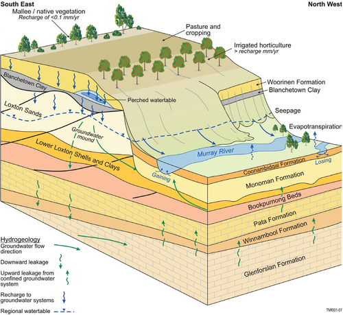
Schematic hydrogeological model of the Bookpurnong floodplain and adjacent highlands. High recharge from irrigation on the highlands adjacent to the flood-plain results in the development of a groundwater mound and an increase in the hydraulic gradient towards the floodplain. A rise in water levels across the floodplain results. Increased evapotranspiration results in the concentration of salt in the near surface soils. These changes also promote the discharge of higher salt loads into the river.
FIELD EXAMPLE: THE BOOKPURNONG SURVEY AREA
Test area and hydrogeology
The Bookpurnong floodplain is located adjacent to the Bookpurnong Irrigation District on the Murray River in the Riverland region of South Australia, see Fig. 6. It has a hydrogeology typical of the eastern part of the lower Murray Basin, see Fig. 7. On the floodplain, the Coonambidgal Clay ranges from 3–7 m thick, while the Monoman Formation is approximately 7 m thick in this area. The cliffs adjacent to the flood-plains consist of a layer of Woorinen Sands over Blanchtown Clay, each approximately 2 m thick, overlying the Loxton Sands, which can be up to 35 m thick. The whole area is underlain by the Bookpurnong Beds, which act as an aquitard basement to the shallow aquifer that encompasses the Monoman Formation and Loxton Sands. Groundwater salinity in the Loxton Sands and Monoman Formation exceeds 30,000 mg/l, while irrigation recharge salinity is typically 5,000 mg/l. Excess recharge from the Bookpurnong Irrigation District has led to the formation of a groundwater mound, which displaces saline groundwater towards the floodplain and has led to increased waterlogging and salinization on the floodplain. Groundwater seepage occurs at the break of slope adjacent to the cliffs. In places, Black Box (Eucalyptus largiflorens) and Red Gum (E. camaldulensis) tree communities have been severely affected by the salinization of the floodplain. On the floodplain, there is considerable variation of evapotranspiration and seepage depending on distribution of soils, vegetation type, floodplain elevation and geometry.
The Bookpurnong FDHEM data
The Bookpurnong FDHEM survey was flown by Fugro Airborne Surveys with the RESOLVE® helicopter-borne frequency domain system during the period 1–9 July 2005. Survey speed was 80–120 km/h and data were sampled every 0.1 s corresponding to a sounding for every  m along the profiles. Line spacing was 100 m with tie-lines for every 1 km. The data used in this study were calibrated against conductivity logs in the area after standard levelling and calibration using a procedure described by Brodie et al. (2004).
The FDHEM data set comprises the real and imaginary – or inphase  and quadrature
  – of the six frequencies of the system. Five frequencies are in the horizontal coplanar configuration and one is in the vertical coaxial configuration. Only the horizontal coplanar configurations have been used in this study. The noise levels ascribed to the data before inversion are taken from the contractor’s report (Fugro Airborne Surveys 2005) and defined as half of the peak-to-peak noise levels after data processing. Table 2 summarizes the system parameters.
Inversion, data fit and data inconsistency
In general, most of the soundings can be interpreted well with 1D models with typical values of the residuals of the order of 1–3. This indicates that we are on the safe side with regard to fitting noise, which was also our intention when we chose the regularization level on the conservative side. At certain locations, primarily where rapid changes in topography are present, inconsistency with the assumption of a 1D model will result in a poorer data fit. In some of these locations, it appears that the topographical variation is caused by insufficient height processing. The digital terrain model is derived as the helicopter GPS altitude minus a constant standard cable length and minus the bird height. Errors in bird height will thus be transferred to the terrain model.
Presentation of results: model sections
For every one of the 26 survey lines and the 7 tie-lines, the models resulting from inversion of the individual sounding data are concatenated in model sections, plotted with easting as profile parameter. The top plot in the model sections shows the inverted models with topography where the resistivity of the individual layers are colour coded on a logarithmic scale according to the colour bar. The bird height is also indicated in the model sections. Below the model section is a plot of the residuals of the inversions: blue indicates the data residual and black is the total residual. For reasons of space, we shall show model sections of only the two adjacent lines 20160 and 20170, which are seen in Fig. 8.
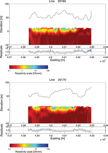
Model sections of concatenated 1D models from Line 20160 and Line 20170.
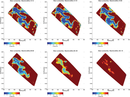
Colour contoured maps of mean conductivity in the elevation intervals: 14 m to 12 m, 12 m to 10 m, 10 m to 5 m, 5 m to 0 m, 0 m to –5 m and –5 m to –10 mAHD.
Both lines are from the southern part of the survey area and traverse across the floodplain, crossing first a small anabranch in the westernmost part of the survey area after which they intersect the Murray River five times. Line 20160 shows the anabranch and the resistive freshwater part just outside of a lobe of the anabranch while Line 20170 crosses it twice. In Line 20160 the first crossing of the Murray River at easting 460.4 is clearly separated from the subsequent two river crossings by a conductive area indicating a saline environment. Traversing south-east, the third river crossing is separated from the fourth river crossing by another conductive feature. The fifth river crossing at easting 462.5 is not accompanied by any resistive feature indicating a saline river and environment. In Line 20170 the resistive features of the four river crossings are smeared together by the resistive river environment indicating that freshwater is lost from the river but again the fifth river crossing is conductive. The similarity between the two profile lines testify to the reliability of the data and the inversion method and the differences indicate rapid changes in the salinity of the environment and that they are reasonably resolved by the data and their interpretation.
All model sections appear laterally smooth even though inversion was done on every data set individually. Lateral constraints in the inversion were unnecessary due to the lateral smoothing of the data effected by the contractor.
Presentation of results: contoured maps of mean conductivity
 is defined as
 (18)
(18)where the latter expression is valid for a layered earth model with  layers. The weight factor,
  , is the thickness of the part of the layer lying within the elevation interval
  . For reasons of space, we show model sections of only six elevation intervals, which are seen in Fig. 9.
Figure 9 shows that the resistive features associated with lateral bank recharge of fresh river water around the Murray River disappear with decreasing elevation, as the saline groundwater system is encountered at depth. It is also seen that the weak and narrow resistive areas around the most south-eastern bend of the river that are seen in the two uppermost intervals disappear completely after the third elevation interval.
COMPARISON BETWEEN THE FAST APPROXIMATE INVERSION, CONVENTIONAL INVERSION AND EMFLOW
In Fig. 10, model sections for Line 60010 derived from fast approximate inversion, conventional inversion and EMflow are shown. For the fast approximate and conventional inversion, the initial model, the regularization and all other inversion parameters were identical. Limited difference is observed between the two sections. There is a weak tendency for the fast approximate inversion to enhance the conductive features slightly. The EMflow section is similar to the two inverted sections but the implicit regularization in EMflow appears to result in weaker constraints than the explicit one used in the inversions. Referring to Fig. 5, the EMflow section shows greater similarities to the fast approximate inversions section for a model covariance standard deviation of  rather than the value
  chosen for the inversion of the whole survey. At profile coordinate 462500 there seems to be a discontinuity in the EMflow model section and, in general, the bottom layer resistivity appears to be poorly constrained. The EMflow model section is shown without a residual plot because EMflow does not define a data residual.
Computation times for the approximate inversion, the conventional inversion and the EMflow processing of the 791 data sets on Line 60010 are seen in Table 3 below. On average, the fast approximate inversion is 30 times faster than the conventional inversion but EMflow is considerably faster.
| Inversion type | Total time (s) | Total time per sounding (s) |
|---|---|---|
| Conventional | 2673.88 | 3.38 |
| Approximate | 87.98 | 0.11 |
| EMflow | 2 | 0.0026 |
In Fig. 11, colour contoured maps of the mean conductivity in the elevation interval from 10 – 5 mAHD are shown based on the fast approximate inversion, the conventional inversion and the EMflow processing. In the north-western and central parts of the survey area, flushed zones represented as resistive freshwater saturated areas around the river are visible, whereas in the south-eastern corner flushed zones are replaced by conductive areas adjacent to the river, representing zones where saline groundwater is discharging into the river through the river bed sediments and via its banks. There are limited differences between the two maps from the fast and conventional inversion, except for the above-mentioned tendency of the fast inversion to slightly enhance the conductive features. The map derived from the EMflow processing is also similar to the maps from the inversion procedures.
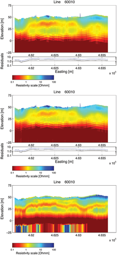
Comparison between fast approximate inversion (top) and conventional inversion (middle) of Line 60010. All inversion settings were identical for the two sections. The bottom model section is derived from EMflow processing of the data.
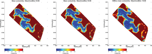
Comparison between contoured maps of mean conductivity in the elevation interval 10– 5 m based on the fast approximate inversion (left), the conventional inversion (middle) and the EMflow processing (right).
 (19)
(19) is the number of data, while the total residual also involves the deviation between the initial prior model and the final model and it is defined as
 (20)
(20)where  is the number of layers in the MLM.
Below, in Table 4, is a comparison of the mean residual and its standard deviation for the approximate inversion, the conventional inversion and the conventional forward responses of the models obtained from the approximate inversion. It is seen that, on average, the approximate and conventional inversion both stop at residuals around 3 and that the residuals corresponding to the conventional responses of the models found in the approximate inversion are 75% higher than the residuals of the conventional inversion, i.e., not even doubled.
| Inversion type | Mean value | Standard deviation |
|---|---|---|
| Approximate | 3.01 | 0.79 |
| Conventional | 3.05 | 0.89 |
| Conventional response of approximate models | 5.38 | 1.97 |
Correlation with borehole logs
In Fig. 12, the inversion results of the approximate and conventional inversion and the EMflow results are compared with the conductivity measured by an induction log in boreholes GDN141 and BH007 (see Fig. 6 for locations of bores). The borehole GDN141 is located at (E461670, N6200199) and BH007 at (E463320, N6201100) and the inversion results have been taken from the fiducial located closest to the boreholes.
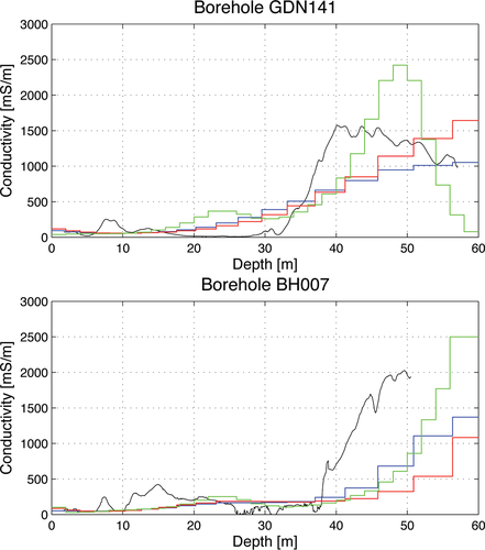
Comparison between the subsurface conductivity measured by an induction logging tool (black curve) and the conductivities of the inverted models of the fast approximate inversion (red), the conventional inversion (blue) and the EMflow results (green) for the boreholes GDN141 and BH007. See Fig. 6 for locations of bores.
The comparison shows, in general, good agreement between the measured conductivity logs and the two inversion results and the EMflow processing and confirms the similarity between the inversions and the EMflow results. In GDN141, the EMflow conductivity rises faster to indicate the increase in conductivity of the log, probably because of the implicit weaker regularization of the EMflow processing mentioned before. Above the bulge peak, profiles show good shape agreement with models, although conductivity is overestimated. Below the peak, profiles taper and modelled conductivity is underestimated. This behaviour has been described by Hunter and Macnae (2001).
DISCUSSION AND CONCLUSIONS
We have presented a fast approximate inversion procedure for FDHEM data and applied it to the Bookpurnong RESOLVE® survey from South Australia. The fast approximate inversion is based on a fast approximate forward mapping, which in turn is found through Fourier transformation of fast approximate TEM step responses. Likewise, the derivatives used in the inversion are found as Fourier transformation of the corresponding approximate TEM derivatives. The fast approximate inversion is about 30 times faster than conventional 1D inversion using identical initial models and regularization
The inversion is implemented using an iterative, constrained least squares inversion formulation for multi-layer models. The inversion is regularized using a broadband model covariance matrix and the strength of the regularization is pragmatically chosen based on inspection of inversion results from selected profile lines for different settings.
The model sections and contoured maps of mean conductivity in elevation intervals constructed from the inversion of the Bookpurnong data set reveal the distribution of salinity in the survey area and indicates where the Murray River looses freshwater to the surroundings and where saline groundwater discharges into the river. Arguably, this information is crucial for any remediation efforts aimed at reducing the salinization of the river.
Comparisons between approximate and conventional forward responses for four principal models for a FDHEM system indicate that the fast approximate inversion is modelling the ground conductivity reasonably well. Residuals between the approximate and conventional forward response for the series of three-layer test models are below 5% for a resistive middle layer for any contrast and below 10% for a conductive middle layer, provided that the resistivity contrast is less than a factor of 15. The inversion of theoretical data from the series of test models gives very similar results for the approximate and conventional inversion.
A comparison of model sections from the approximate and the conventional inversion of field data shows very little difference; they are almost indistinguishable from one another as are the maps of mean conductivity in elevation intervals. On average, the misfit between data and conventional forward responses of the models found in the approximate inversion is only  % higher than that of the conventional inversion results.
A comparison with the results of EMflow processing of the data from Line 60010 shows that EMflow performs well for these data. The EMflow model section is very similar to the model sections from the inversions but has a weaker implicit regularization. Also the map of mean conductivity in the elevation interval 10–5 m is very similar to the maps obtained from the inversions. Comparison with borehole induction conductivity log shows, in general, good agreement for all methods.
Considering the similarity between the results of the approximate and conventional inversion and that the approximate inversion is 30 times faster, it can be concluded that the approximate inversion technique offers an attractive alternative to conventional inversion techniques. In cases where the emphasis is on structural information, model sections and mean conductivity maps derived from the approximate inversion will suffice and there is no need for conventional full inversion. In cases where the depth to layers boundaries between layers of sharp conductivity contrasts is needed, few-layer inversion must be carried out. The approximate inversion cannot be used in few-layer, parametric inversion but excellent starting models for the few-layer inversion can be inferred from the multi-layer models of the approximate inversion, thus ensuring stable convergence and considerably reducing computation time.
The fast approximate inversion makes it possible to invert data in the field as soon as they are transferred from the instrument. Provided that data are reasonably calibrated, an appropriately robust data processing followed by an approximate inversion with robust regularization enables the contractor and client to examine the results of the measurements the same day the data are recorded. As far as the survey contract permits, this enables daily changes to be made to the survey strategy and layout.
Fast approximate inversion will always be useful no matter how fast computers will become because the number of measured data and the complication level of the processing and inversion also increase in proportion with the computer speed. A colleague of ours recently suggested that the time used on the physical interpretation, i.e., the inversion of processed data, was inconsequential compared with the time required for a conscientious data processing and, in particular, the time spent after the inversion on the geological/hydrogeological interpretation of the inversion results. We would have to agree with that. It is obvious that an increase in inversion speed with a factor of 30 does not mean that the whole interpretation process increases with the same factor. However, the fast inversion offers itself as an integral part of a well formulated inversion strategy and it is indispensable for quality control in the field and an adaptive measuring strategy.
ACKNOWLEDGEMENTS
This paper reflects a collaborative research effort between the Hydrogeophysics Group of the University of Aarhus, Denmark and the CSIRO Flagship: Water for a Healthy Country, aimed at developing and testing new inversion techniques to predict conductivity responses of the ground from airborne EM systems. This work has been supported by the South Australian Governments Centre for Natural Resource Management (Project #054127) and the CSIRO Flagship Water for a Healthy Country through the Better Basins Future Theme.
APPENDIX: Fast approximate inversion of TEM data
Approximate forward mapping
The fast approximate inversion in the frequency domain is based on a fast approximate forward mapping in the time-domain from conductivity as a function of depth to step response for a 1D layered model:  (Christensen 2002). This forward mapping consists in two consecutive mappings: 1) a mapping from conductivity as a function of depth to apparent conductivity as a function of time:
  , followed by 2) a substitution of the apparent conductivity into a half-space response:
  . The step response for a layered model is by definition given as the half-space response at the same delay time for a half-space conductivity equal to the apparent conductivity. The first mapping,
  , is generic, i.e., it is the same for all transmitter-receiver (Tx-Rx) configurations and field components. In the second mapping,
  , the half-space response is specific for the configuration and field component in question. However, they need only be calculated once at program start. In the case of airborne systems, a half-space response must be calculated for a series of heights with a proper density to allow accurate interpolation.
 (21)
(21)where  is a weight function that depends on the apparent conductivity. In this way the slower diffusion through good conductors and the faster diffusion through poor conductors are taken into account, i.e., the mapping is model adaptive.
 layers with conductivities
  and upper layer boundaries
  ,
, 
 (22)
(22) is the integrated weight function
 (23)
(23) (24)
(24) (25)
(25)which is a different choice from the linear function used in Christensen (2002). Many different weight functions will be equally good but, as opposed to the linear weight function in Christensen (2002), the one defined above has continuous derivatives that make it perform better in some situations. The parameter  scales the depth extent of the sensitivity function and eventually the depth scaling of the resulting models after inversion. It is chosen to minimize the difference between a series of test models and the approximate inversion results (Christensen 2002).
Substituting the apparent conductivity into the half-space step response, we have computed the layered step response  .
.

 and not of
  and
and  independently, so
 (27)
(27)Derivatives with respect to layer thicknesses can be expressed in terms of derivatives with respect to conductivity (Christensen 2002) but the fast approximate inversion is used only for multilayer models for which only derivatives with respect to conductivity are relevant.


 are given as

