Quantile treatment effects in difference in differences models with panel data
Abstract
This paper considers identification and estimation of the Quantile Treatment Effect on the Treated (QTT) under a straightforward distributional extension of the most commonly invoked Mean Difference in Differences Assumption used for identifying the Average Treatment Effect on the Treated (ATT). Identification of the QTT is more complicated than the ATT though because it depends on the unknown dependence (or copula) between the change in untreated potential outcomes and the initial level of untreated potential outcomes for the treated group. To address this issue, we introduce a new Copula Stability Assumption that says that the missing dependence is constant over time. Under this assumption and when panel data is available, the missing dependence can be recovered, and the QTT is identified. We use our method to estimate the effect of increasing the minimum wage on quantiles of local labor markets' unemployment rates and find significant heterogeneity.
1 Introduction
Although most research using program evaluation techniques focuses on estimating the average effect of participating in a program or treatment, in some cases a researcher may be interested in understanding the distributional impacts of treatment participation. For example, for two labor market policies with the same mean impact, policymakers are likely to prefer a policy that tends to increase income in the lower tail of the income distribution to one that tends to increase income in the middle or upper tail of the income distribution. In contrast to the standard linear model, the treatment effects literature explicitly recognizes that the effect of treatment can be heterogeneous across different individuals (Heckman and Robb (1985), Heckman, Smith, and Clements (1997)). Recently, many methods have been developed that identify distributional treatment effect parameters under common identifying assumptions such as selection on observables (Firpo (2007)), access to an instrumental variable (Abadie, Angrist, and Imbens (2002), Chernozhukov and Hansen (2005), Carneiro and Lee (2009), Frolich and Melly (2013)), or access to repeated observations over time (Athey and Imbens (2006), Bonhomme and Sauder (2011), Chernozhukov, Fernandez-Val, Hahn, and Newey (2013), Jun, Lee, and Shin (2016)). This paper focuses on identifying and estimating a particular distributional treatment effect parameter called the Quantile Treatment Effect on the Treated (QTT) using a Difference in Differences Assumption for identification.
Empirical researchers commonly employ Difference in Differences Assumptions to credibly identify the Average Treatment Effect on the Treated (ATT) (early examples include Card (1990), Card and Krueger (1994)). Despite the prevalence of DID methods in applied work, there has been very little empirical work studying the distributional effects of a treatment with identification that exploits having access to repeated observations over time (Recent exceptions include Meyer, Viscusi, and Durbin (1995), Finkelstein and McKnight (2008), Pomeranz (2015), Havnes and Mogstad (2015)).
The first contribution of the current paper is to provide identification and estimation results for the QTT under a straightforward extension of the most common mean Difference in Differences Assumption (Heckman and Robb (1985), Heckman, Ichimura, Smith, and Todd (1998), Abadie (2005)). In particular, we strengthen the assumption of mean independence between (i) the change in untreated potential outcomes over time and (ii) whether or not an individual is treated to full independence. We call this assumption the Distributional Difference in Differences Assumption.
For empirical researchers, methods developed under the Distributional Difference in Differences Assumption are valuable precisely because the identifying assumptions are straightforward extensions of the mean Difference in Differences assumptions that are frequently employed in applied work. This means that almost all of the intuition for applying a difference in differences method for the ATT will carry over to identifying the QTT using our method.
Although applying a mean Difference in Differences Assumption leads straightforwardly to identification of the ATT, using the Distributional Difference in Differences Assumption to identify the QTT faces some additional challenges. The reason for the difference is that mean difference in differences exploits the linearity of the expectation operator. In fact, with only two periods of data (which can be either repeated cross sections or panel) and under the same Distributional Difference in Differences Assumption considered in the current paper, the QTT is known to be partially identified (Fan and Yu (2012)) without further assumptions. In practice, these bounds tend to be quite wide. Lack of point identification occurs because the dependence (or copula) between (i) the change in untreated potential outcomes for the treated group and (ii) the initial level of untreated potential outcomes for the treated group is unknown. For identifying the ATT, knowledge of this dependence is not required and point identification results can be obtained.
To move from partial identification back to point identification, we introduce a new assumption which we call the Copula Stability Assumption. This assumption says that the copula, which captures the unknown dependence mentioned above, does not change over time. To give an example, consider the case where the outcome of interest is earnings. The Copula Stability Assumption says that if we observe in the past that the largest earnings increases tended to go to those with the highest earnings, then, in the present (and in the absence of treatment), the largest earnings increases would have gone to those with the highest earnings. Importantly, this does not place any restrictions on the marginal distributions of outcomes over time allowing, for example, the outcomes to be nonstationary. There are two additional requirements for invoking this assumption relative to the mean Difference in Differences Assumption: (i) access to panel data (repeated cross sections is not enough) and (ii) access to at least three periods of data (rather than at least two periods of data) where two of the periods must be pretreatment periods and the third period is post-treatment. We show that the additional requirements that the Copula Stability Assumption places on the type of model that is consistent with the Distributional Difference in Differences Assumption are small.
Based on our identification results, estimation of the QTT is straightforward and computationally fast. Estimating the QTT relies only on estimating unconditional moments, empirical distribution functions, and empirical quantiles. We show that our estimator of the QTT converges to a Gaussian process at the parametric rate  and prove that the empirical bootstrap can be used to approximate this limiting process. This result allows us to conduct uniform inference over a range of quantiles and to test, for example, whether the distribution of treated potential outcomes stochastically dominates the distribution of untreated potential outcomes.
The second contribution of the paper is to extend the results to the case where the identifying assumptions hold conditional on covariates. Here, we consider two cases. First, we consider the combination of a Conditional Difference in Differences Assumption and Unconditional Copula Stability Assumption. We show that that this setup is consistent with a quantile regression-type model for untreated potential outcomes. In this case, we provide very simple estimators for the QTT that are based on a first-step estimation of the propensity score. Second, we consider the combination of a Conditional Difference in Differences Assumption and Conditional Copula Stability Assumption. This setup can allow for trends in untreated potential outcomes to depend on covariates as is also the case for conditional mean Difference in Differences assumptions (Heckman et al. (1998), Abadie (2005)). Estimation is more challenging in this case though as it requires estimating conditional distribution and conditional quantile functions directly.
We conclude the paper by analyzing the effect of increasing the minimum wage on quantiles of the unemployment rates of local labor markets. Despite the average effect of increasing the minimum wage on the unemployment rate being close to 0, using our method, we find that the average effect masks substantial heterogeneity. The difference between the 10th percentile of unemployment among counties that had higher minimum wages and the 10th percentile of counterfactual unemployment had they not had higher minimum wages is negative. However, the effect is quite different elsewhere in the distribution. At the median and upper quantiles, the effect is positive. As long as counties do not change their ranks (or at least do not change their ranks too much) in the distribution of unemployment rates due to the increase in the minimum wage, these results indicate that counties with tight labor markets experienced decreases in the unemployment rate following the minimum wage increase while counties with higher unemployment rates experienced more unemployment due to the increase in the minimum wage. We find similar results using alternative methods such as Quantile Difference in Differences and Change in Changes (Athey and Imbens (2006)).
Because we focus on nonparametric identifying assumptions, the current paper is related to the literature on nonseparable panel data models (Altonji and Matzkin (2005), Evdokimov (2010), Bester and Hansen (2012), Graham and Powell (2012), Hoderlein and White (2012), Chernozhukov et al. (2013)). The most similar of these is Chernozhukov et al. (2013) which considers a nonseparable model and, similar to our paper, obtains point identification for observations that are observed in both treated and untreated states. Relative to Chernozhukov et al. (2013), we exploit having access to a control group much more and our setup is compatible with more complicated distributional shifts in outcomes over time such as the top of the income distribution increasing more than the bottom of the income distribution.
Perhaps the most similar work to ours is Athey and Imbens (2006). Their Change in Changes model identifies the QTT for models that are monotone in a scalar unobservable. They assume that the distribution of unobservables does not change over time (though the distribution of unobservables can be different for the treated group and untreated group) but allow for the return to unobservables to change over time. One advantage of their approach relative to ours is that it only requires two periods of data. However, our main assumptions are more closely related to DID assumptions that are frequently invoked in empirical work.
2 Background
The setup and notation used in this paper is common in the statistics and econometrics literature. We consider a panel data case where the researcher has access to at least three periods of data for all agents in the sample; we denote the three periods by t,  , and
, and  . We focus on the case of a binary treatment. We also focus, as is common in the difference in differences literature, on the case where no one receives treatment before the final period which simplifies the exposition; a similar result for a subpopulation of the treated group could be obtained with little modification in the more general case. Let
  for individuals that are treated at time t (we suppress an individual subscript i throughout much of the paper to minimize notation)—these individuals form the treated group—and let
  for individuals that are never treated. The researcher observes outcomes
  ,
,  , and
, and  for each individual in each time period. The researcher also possibly observes some covariates X.
 and
and  , respectively. The fundamental problem is that exactly one (never both) of these outcomes is observed for a particular individual. Using the above notation, the observed outcome
  can be expressed as follows:


For any particular individual, the unobserved potential outcome is called the counterfactual. The individual's treatment effect,  , is therefore never available because only one of the potential outcomes is observed for a particular individual. Instead, the literature has focused on identifying and estimating various functionals of treatment effects and the assumptions needed to identify them.
In cases where (i) the effect of a treatment is thought to be heterogeneous across individuals and (ii) understanding this heterogeneity is of interest to the researcher, estimating distributional treatment effects such as quantile treatment effects is likely to be important. Comparing the distribution of observed outcomes to a counterfactual distribution of untreated potential outcomes is a very important ingredient for evaluating the effect of a program or policy (Sen (1997), Carneiro, Hansen, and Heckman (2001)) and provides more information than the average effect of the program alone. For example, a policy maker may be in favor of implementing a job training program that increases earnings for individuals in the lower tail of the distribution of earnings while decreasing earnings of those in the the upper tail of the distribution of earnings even if the average effect of the program is zero.
 , of W is defined as

 denotes the distribution of W. An example is the 0.5-quantile—the median.2 Researchers interested in program evaluation may be interested in other quantiles as well. For example, researchers studying a job training program may be interested in the effect of the program on low income individuals. In this case, they may study the 0.05 or 0.1-quantile. Similarly, researchers studying the effect of a policy on high earners may look at the 0.95-quantile.
 and
and  denote the distributions of
  and
and  conditional on being in the treated group, respectively. Then the Quantile Treatment Effect on the Treated (QTT)3 is defined as

3 Identification
Let  denote the time difference in untreated potential outcomes. The most common nonparametric assumption used to identify the ATT in difference in differences models is the following.
Assumption 3.1. (Mean difference in differences)

This is the “parallel trends” assumptions that is common in applied research. It states that, on average, the unobserved change in untreated potential outcomes for the treated group is equal to the observed change in untreated outcomes for the untreated group. To study the QTT, Assumption 3.1 needs to be strengthened because the QTT depends on the entire distribution of untreated outcomes for the treated group rather than only the mean of this distribution.
The next assumption strengthens Assumption 3.1 and this is the assumption maintained throughout the paper.
Distributional Difference in Differences Assumption.

The Distributional Difference in Differences Assumption says that the distribution of the change in untreated potential outcomes does not depend on whether or not the individual belongs to the treated or the untreated group. Intuitively, it generalizes the idea of “parallel trends” holding on average to the entire distribution. In applied work, the validity of using a difference in differences approach to estimate the ATT hinges on whether the unobserved trend for the treated group can be replaced with the observed trend for the untreated group. This is exactly the same sort of thought experiment that needs to be satisfied for the Distributional Difference in Differences Assumption to hold. Being able to invoke a standard assumption to identify the QTT stands in contrast to the existing literature on identifying the QTT in similar models which generally require less familiar assumptions on the relationship between observed and unobserved outcomes.
Using statistical results on the distribution of the sum of two random variables with known marginal distributions but unknown copula, Fan and Yu (2012) showed that this assumption is not strong enough to point identify the counterfactual distribution  , but it does partially identify it. In practice, these bounds tend to be very wide—too wide to be useful in most applications.
3.1 Main results: Identifying QTT in difference in differences models
The main theoretical contribution of this paper is to impose a Distributional Difference in Differences Assumption plus additional data requirements and an additional assumption that may be plausible in many applications to identify the QTT. The additional data requirement is that the researcher has access to at least three periods of panel data with two periods preceding the period where individuals may first be treated. This data requirement is stronger than is typical in most difference in differences setups which usually only require two periods of repeated cross-sections (or panel) data. The additional assumption is that the dependence—that is, the copula4—between (i) the change in untreated potential outcomes for the treated group and (ii) the initial level of untreated potential outcomes for the treated group is stable over time. This assumption says that if, in the past, the largest increases in outcomes tend to go to those initially at the top of the distribution, then in the present, the largest increases in outcomes will tend to go to those who start out at the top of the distribution. It does not restrict what the distribution of the change in outcomes over time is nor does it restrict the distribution of outcomes in the previous period; instead, it restricts the dependence between these two random variables. We discuss this assumption in more detail and show how it can be used to point identify the QTT below.
Intuitively, the reason why a restriction on the dependence between  and
and  is useful is the following. If the joint distribution
  were known, then
  (the distribution of interest) could be derived from it. The marginal distributions
  (through the Distributional Difference in Differences Assumption) and
  (from the data) are both identified. However, because observations are observed separately for untreated and treated individuals, even though each of these marginal distributions are identified, the joint distribution is not identified. Since, from Sklar's theorem (Sklar (1959)), joint distributions can be expressed as the copula function (capturing the dependence) of the two marginal distributions, the only piece of information that is missing is the copula.5 We use the idea that the dependence is the same between period t and period
  . With this additional information,
  is identified and, therefore, the counterfactual distribution of untreated potential outcomes for the treated group,
  , is identified.
 and
and  can be expressed in the following way. Let
  be the joint distribution of
  and
and  for the treated group. By Sklar's theorem,
 (1)
(1) is a copula function.6 Next, we state the second main assumption which replaces the unknown copula with the copula for the same outcomes but in the previous period which is identified because no one is treated in the periods before t.
Copula Stability Assumption.

The Copula Stability Assumption says that the dependence between  and
and  is the same as the dependence between
  and
and  . It is important to note that this assumption does not require any particular dependence structure, such as independence or perfect positive dependence; rather, it requires that whatever the dependence structure is in the past, one can recover it and reuse it in the current period. It also does not require choosing any parametric copula. However, it may be helpful to consider a simple, more parametric example. If the copula of
  and
and  is Gaussian with parameter ρ, the Copula Stability Assumption says that the copula continues to be Gaussian with parameter ρ in period t but the marginal distributions are allowed to change in unrestricted ways. Likewise, if the copula is Archimedean, the Copula Stability Assumption requires the generator function to be constant over time but the marginal distributions can change in unrestricted ways.
One of the key insights of this paper is that, in some particular situations such as the panel data case considered in the paper, we are able to observe the historical dependence between the marginal distributions. There are many applications in economics where the missing piece of information for identification is the dependence between two random variables. In those cases, previous research has resorted to (i) assuming some dependence structure such as independence or perfect positive dependence or (ii) varying the copula function over some or all possible dependence structures to recover bounds on the joint distribution of interest. To our knowledge, we are the first to use historical observed outcomes to obtain a historical dependence structure and then assume that the dependence structure is stable over time.
Before presenting the identification result, we need some additional assumptions. First, let  . Let
. Let  denote the support of the change in outcomes for the untreated group in period t. Let
  ,
,  , and
, and  denote the support of the change in outcomes for the treated group in period
  , the support of outcomes for the treated group in period
  , and the support of outcomes for the treated group in period
  , respectively. And let
  denote the support of X.
Assumption 3.2.Each of the random variables  for the untreated group and
  ,
,  , and
, and  for the treated group are continuously distributed on their support with densities that are uniformly bounded from above and bounded away from 0.
Assumption 3.3.The observed data  are independent and identically distributed draws from the joint distribution
  ; and
; and  ,
,  , and
, and  .
.
Assumption 3.2 says that outcomes are continuously distributed. Copulas are unique on the range of their marginal distributions; thus, continuously distributed outcomes guarantee that the copula is unique. However, for the Copula Stability Assumption, one could weaken this assumption to  and
and  and still obtain point identification. On the other hand, although neither our Distributional Difference in Differences Assumption nor the standard mean DID assumption explicitly require continuously distributed outcomes, it should be noted that standard limited dependent variable models with unobserved heterogeneity would not generally satisfy either of these DID assumptions. Assumption 3.3 says that we are in the case with panel data, and that no one is treated in the first two periods. Assumption 3.3 could potentially be relaxed in several ways. More periods of data could be available—our method requires at least three periods of data, but more periods could be incorporated (e.g., it seems possible to extend the approach of Callaway and Sant'Anna (2019) for the ATT to our case for the QTT). Also, our setup could allow for some individuals to be treated in earlier periods than the last one and our results would continue to go through for the group of individuals that are first treated in the last period; considering the case where no one is treated before the last period is standard in DID setups. Assumption 3.3 also says that other covariates X are either time invariant or, in the case with time varying covariates, that we condition on pretreatment values of the covariates.7
Theorem 1.Under the Distributional Difference in Differences Assumption, the Copula Stability Assumption, and Assumptions 3.2 and 3.3,


 . This expression is an integral over the joint distribution of
  and will be identified when the joint distribution is identified. Under the Distributional Difference in Differences Assumption, this joint distribution is not identified (though the marginals are), but the Copula Stability Assumption replaces the unknown copula in Equation (1) with the observed copula for the treated group in the previous period which leads to the identification result. Replacing the unknown copula with a copula from the past is what increases the required number of periods from two to three.9 The particular form of the result in Theorem 1 arises from using the dependence structure in period
  (notice that the expectation is over
  and
and  ). The terms of the form
  “adjust” forward outcomes from the previous period and account for the marginal distributions changing over time. Finally, the Distributional Difference in Differences Assumption allows us to replace
  with
with  which is just the quantiles of the distribution of the change in (observed) untreated outcomes for the untreated group.
The following example shows what additional conditions need to be satisfied for our model to be valid in a standard DID setup.
Example 1.Consider the following baseline model for Mean DID:

 is a time fixed effect that is common for the treated and untreated groups,
  is individual heterogeneity that may be distributed differently across the treated group and untreated group, and
  are time varying unobservables. For mean DID to identify the ATT, it must be the case that
  . Sufficient conditions for the assumptions in our model to hold are (i)
  and (ii)
  .
.Condition (i) just strengthens Mean DID to Distributional Difference in Differences. Condition (ii) implies that the Copula Stability Assumption will hold. An interesting sufficient condition for Condition (ii) is  and
and  follow the same distribution (this implies Condition (ii) because it implies that the joint distributions
  and
and  are equal). Condition (ii) will also hold automatically if the time varying unobservables are iid. Condition (ii) allows for the distribution of the time varying unobservables to change over time, it allows for serial correlation in the time varying unobservables, and it allows for the time varying unobservables to be correlated with the individual heterogeneity. Each of these are realistic possibilities in applied work.
We prove the validity of the claims in Example 1 in Appendix A. Some comments on Example 1 are in order. For identifying the ATT, the setup in Example 1 is straightforward. However, obtaining quantile treatment effects is much more challenging because the model is nonlinear in this case. Also, notice that Example 1 only imposes modeling assumptions on how untreated potential outcomes are generated. In particular, it does not put any restrictions on how treated potential outcomes are generated (this is true of mean DID as well), and this means that individuals are allowed to select into treatment on the basis of anticipated treated potential outcomes in an unrestricted way; this is in addition to allowing for the distribution of time invariant unobserved heterogeneity in the model for untreated potential outcomes to differ in unrestricted ways between the treated and untreated groups.
It is also worthwhile to compare our approach to alternative approaches to identifying quantile effects in this sort of model. First, one could try to estimate the individual fixed effects, which is the approach generally taken in the fixed effects quantile regression literature.10 Relative to our approach, this would require a large number of time periods and the resulting estimates would have a different interpretation.11 Another idea would be to impose additional independence conditions among the unobservables (e.g., independence between η and the time varying unobservables and that the time varying unobservables are independent over time) and use results that come primarily from the measurement error literature (e.g., Li and Vuong (1998), Evdokimov (2010), Bonhomme and Sauder (2011), Arellano and Bonhomme (2016), Freyberger (2018)). Our approach does not require any of these additional conditions. Finally, under the additional condition that  follows the same distribution as
  , the approach of Chernozhukov et al. (2013) as well as the Change in Changes model (Athey and Imbens (2006)) would hold.12 But this extra condition is substantially stronger; it implies that the distribution of the outcomes can only shift location over time. Condition (ii) is substantially weaker than this and can allow the distribution of untreated potential outcomes to shift in arbitrary ways over time.
4 Allowing for covariates
Having DID assumptions hold conditional on covariates can make them more likely to hold in many applications (Heckman et al. (1998), Abadie (2005), Lechner (2011)). In this section, we consider the case where the Distributional Difference in Differences Assumption holds after conditioning on covariates. We also consider the cases where (i) the Copula Stability Assumption continues to hold unconditionally or (ii) the Copula Stability Assumption also holds after conditioning on covariates. In the first case, we show that the combination of a Conditional Distributional Difference in Differences Assumption plus Unconditional Copula Stability Assumption is consistent with models for untreated potential outcomes that allow for heterogeneous effects of observed covariates; these sorts of models are similar to well-known panel quantile regression models. In the second case, we show that the combination of the Conditional Distributional Difference in Differences Assumption and the Conditional Copula Stability Assumption is consistent with models that allow for the path of untreated potential outcomes to depend on the covariates. This is also an important case. For example, in the context of job training, individuals who participate in job training often have very different background characteristics than the overall population; if the path of earnings depends on things like education or age (and these are distributed differently between the treated group and untreated group), then the Unconditional Distributional Difference in Differences and Unconditional Copula Stability Assumptions are unlikely to hold though the combination of the Conditional Distributional Difference in Differences Assumption and the Conditional Copula Stability Assumption may continue to hold. We make the following assumption throughout this section.
Conditional Distributional Difference in Differences Assumption.

This assumption says that, after conditioning on covariates X, the distribution of the change in untreated potential outcomes for the treated group is equal to the distribution of the change in untreated potential outcomes for the untreated group. This assumption strengthens conditional mean DID assumptions (as in Heckman et al. (1998), Abadie (2005)) from mean independence to full independence. This is analogous to the extension from unconditional mean DID to the Unconditional Distributional Difference in Differences Assumption made in the previous section. The next example shows that having the Conditional Distributional Difference in Differences Assumption may be important even in cases where an unconditional mean DID assumption holds and would identify the ATT.
Example 2.Consider the following model for untreated potential outcomes:

 and
and  where
where  is a bivariate distribution with uniform marginals, η is time invariant unobserved heterogeneity that may be correlated with observables and distributed differently for the treated and untreated groups, and
  is strictly increasing in τ for all
  .
.In this model, (i) the Unconditional Mean Difference in Differences Assumption holds, (ii) the Unconditional Distributional Difference in Differences Assumption does not hold, (iii) the Conditional Distributional Difference in Differences Assumption holds, and (iv) the Unconditional Copula Stability Assumption holds.
In Appendix A, we show that the claims in Example 2 hold. The model in Example 2 includes untreated potential outcomes being generated by panel quantile regression models (e.g., Koenker (2005), Canay (2011)) as a special case while also allowing for serial correlation among U. This model allows the effect of covariates to be different at different parts of the conditional distribution. For example, if Y is earnings, it is well known that the effect of education is different at different parts of the conditional distribution (Angrist, Chernozhukov, and Fernández-Val (2006)). Also, as was the case for Example 1, the model in Example 2 is only for untreated potential outcomes, and this implies that it allows for selection into treatment on the basis of anticipated treated potential outcomes in addition to allowing for the distribution of the time invariant unobserved heterogeneity and covariates to vary between the treated and untreated groups.
Example 2 is a leading case for using distributional methods to understand heterogeneity in the effect of a treatment, and one conclusion to be reached from this example is that even when an unconditional mean DID assumption holds, one may still need to condition on covariates to justify the Distributional Difference in Differences Assumption. On the other hand, in this model, the Unconditional Copula Stability Assumption continues to hold.
By invoking the Conditional Distributional Difference in Differences Assumption rather than the Unconditional Distributional Difference in Differences Assumption, it is important to note that, for the purpose of identification, the only part of Theorem 1 that needs to be adjusted is the identification of  . Under the Unconditional Distributional Difference in Differences Assumption, this distribution could be replaced directly by
  ; however, now we utilize a propensity score reweighting technique to replace this distribution with another object (discussed more below). Importantly, all other objects in Theorem 1 can be handled in exactly the same way as they were previously which is due to the Unconditional Copula Stability Assumption being invoked.
With covariates, we also require an additional standard assumption for identification.
Assumption 4.1. and, for all
  ,
,  .
.
Proposition 1.Under the Conditional Distributional Difference in Differences Assumption, the Copula Stability Assumption, and Assumptions 3.2, 3.3 and 4.1,

 (2)
(2)
This result is very similar to the main identification result in Theorem 1. The only difference is that  is no longer identified by the distribution of untreated potential outcomes for the untreated group; instead, it is replaced by the reweighted distribution in Equation (2). Equation (2) can be understood in the following way. It is a weighted average of the distribution of the change in outcomes experienced by the untreated group. The
  term weights up untreated observations that have covariates that make them more likely to be treated. Equation (2) is almost exactly identical to the reweighting estimators given in Hirano, Imbens, and Ridder (2003), Abadie (2005), Firpo (2007); the only difference is the term
  in our case is given by
  ,
,  , and
, and  in each of the other cases, respectively.
Finally, in this section, we consider identification under the Conditional Distributional Difference in Differences Assumption and under a Conditional Copula Stability Assumption. In particular, we make the following assumption.
Conditional Copula Stability Assumption.For all  ,
,

Example 3.Consider the following model for untreated potential outcomes:

 allows for covariates to affect the path of untreated potential outcomes in ways that can vary over time,
  is individual heterogeneity that can be distributed differently between individuals in the treated and untreated groups, and
  are time varying unobservables. Sufficient conditions for the Conditional Distributional Difference in Differences Assumption and Conditional Copula Stability Assumption to hold are that (i)
  and (ii)
  . In addition, under the same conditions, conditional mean DID holds (this is implied by Conditional Distributional Difference in Differences); however, none of unconditional mean DID, the Unconditional Distributional Difference in Differences Assumption, or the Unconditional Copula Stability Assumption hold.
Proposition 2.Assume that, for all  ,
,  for the untreated group,
  ,
,  , and
, and  for the treated group are continuously distributed conditional on x. Under the Conditional Distributional Difference in Differences Assumption, the Conditional Copula Stability Assumption, and Assumptions 3.2, 3.3 and 4.1


5 Estimation
In this section, we discuss the estimation procedure as well as outline an inference procedure to conduct uniformly valid inference over a range of quantiles using the empirical bootstrap. We provide formal theoretical results for the limiting process of our estimator in Appendix B as well as a formal justification for the use of the empirical bootstrap in Appendix B.


 is the number of observations in the treated group and
  is the set of treated individuals.
To conduct inference, we propose using the empirical bootstrap to construct uniform confidence bands that cover  with fixed probability for all values
  for some small, positive
  . We derive formal results on the limiting process and the validity of the bootstrap for our estimator of the QTT in Appendix B.
 denote an estimate of the QTT using the same steps as above but with a bootstrapped sample (i.e., a sample with n observations drawn from the original sample with equal probabilities and with replacement). Theorem 3, in the Online Supplementary Appendix, shows that the empirical bootstrap can be used to approximate the limiting process of our estimator.13 To obtain uniform confidence bands, let B be the number of bootstrap iterations and for
  calculate

 is estimated using a bootstrapped sample and where
  , which is the bootstrapped interquartile range divided by the interquartile range of a standard normal random variable; this is a uniformly consistent estimator of
  with
with  being the asymptotic variance function of the QTT. Then a
  confidence band is given by

 and where
  is the
  quantile of
  .
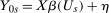
. . Building on the identification result in Proposition 1, we can construct an estimator of the distribution function

 denotes an estimator of the propensity score and where the last term in the denominator normalizes the weights to sum to one in finite samples; it ensures that
  is a distribution function, and this term is asymptotically negligible. One can invert this distribution to obtain its quantiles. We provide formal results on the limiting process for the QTT and the validity of the empirical bootstrap in the Online Supplementary Appendix where we allow for both parametric and nonparametric estimators of the propensity score and provide high level conditions for the estimator of the propensity score that can be satisfied by other estimators (e.g., semiparametric estimators) under some regularity conditions.
In the case considered in Proposition 2, estimation is potentially substantially more challenging. Nonparametric estimation would require estimating five conditional distribution or conditional quantile functions which is likely to be infeasible in many applications (particularly in the case with a relatively large number of covariates and moderate number of observations). In subsequent work (Callaway, Li, and Oka (2018)), we considered a conditional copula assumption in a related model in the case where all the covariates are discrete. Those inference results are likely to continue to go through with minor adaptations to the current model in the particular case with only discrete covariates. Another idea is to estimate the conditional distributions and conditional quantiles using parametric quantile regressions. Melly and Santangelo (2015) use quantile regression to estimate a conditional version of the Change in Changes model (Athey and Imbens (2006)); Wuthrich (2018) uses a similar approach to estimate quantile treatment effects with endogeneity. It seems likely that one could adapt their inference results to our case in a straightforward way as well.
6 Application
In this section, we use our method to study the effect of increasing the minimum wage on county-level unemployment rates. There is a wide body of research that studies the effect of the minimum wage on employment exploiting policy changes across states (e.g., Neumark and Wascher (1992), Dube, Lester, and Reich (2010), among many others). Like most of the literature, we use variation in state-level changes in the minimum wage. Also, we suppose that there may be time invariant differences in the unemployment rate across counties that cannot be accounted for by observable differences in county characteristics. This implies that a DID approach should be used and is in line with much of the literature on minimum wage increases.
The aim of this section is different from most research on the effect of increasing the minimum wage. The literature almost exclusively looks at the average effect, or the coefficient in a linear regression model, of increasing the minimum wage on employment for teenagers, restaurant workers, or some other subgroup. Instead, by looking at the QTT, we examine how the effect of increasing the minimum wage varies by the strength of a county's local labor market. In other words, we ask the question: What is the distribution of unemployment rates across counties following a minimum wage increase relative to what it would have been if the minimum wage had not been increased? This goal is also different from trying to understand the effect of minimum wage increases at different parts of the individual income distribution as in Dube (2017).
Unlike most of the literature on minimum wages, instead of using a long panel of counties, states, and many changes in minimum wage policy across states; we focus on a particular period where the federal minimum wage was flat while there was variation in state minimum wages. The U.S. federal minimum wage increased from $4.25 to $5.15 between 1996 and 1997. It did not increase again until the Fair Minimum Wage Act was proposed on January 5, 2007 and enacted on May 25, 2007. The Act increased the federal minimum wage to $5.85 on July 24, 2007, and increased the minimum wage in two more increments, settling at $7.25 in July of 2009.
In 2006, there were 33 states for whom the federal minimum wage was the binding minimum wage in the state. Of these, we drop two states—New Hampshire and Pennsylvania—because they are located in the Northern census region; census region is an important control in the minimum wage literature (Dube, Lester, and Reich (2010)) and almost all states in the Northern census region had minimum wages higher than the federal minimum wage by 2006. Of the remaining states, 11 increased their minimum wage by the first quarter of 2007—these states form our treated group.14 The other 20 did not increase their minimum wage until the federal minimum wage increased in July of 2007.15
County level unemployment rates are the outcome variable. We obtain these from the Local Area Unemployment Statistics Database from the Bureau of Labor Statistics. Unemployment rates are available monthly and we use unemployment rates in February as the outcome variable. We choose February instead of January because it does not overlap with the holidays and choose it over later months because it is further away from the federal minimum wage change in July. We also merge in county characteristics from the 2000 County Data Book. In our application, these include 2000 county population and 1997 county median income. We collected data for each year from 2000–2007. Our method requires three periods of data, but the earlier periods allow us to pretest our model in earlier periods.
Table 1 provides summary statistics. From 2005–2007, the level of unemployment rates is higher for treated counties than for untreated counties. The gap narrows from 2005 to 2006, the period before any counties have increased minimum wages, and then expands again from 2006 to 2007; this may provide some suggestive evidence that the minimum wage is increasing unemployment rates on average. Counties that are treated are also different from untreated counties in terms of their observable characteristics. Treated counties are more likely to be in the West and North Central regions while untreated counties are more likely to be in the South. Median incomes are very similar (though statistically different) across treated and untreated counties. And treated counties tend to be more populated; log population of 10.34 for treated counties is almost  while log population of 9.91 for untreated counties is just over
  .
.
|
Treated counties |
Untreated counties |
Diff |
P-val on diff |
|
|---|---|---|---|---|
|
Unemployment rate 2007 |
6.10 |
5.07 |
1.028 |
0.00 |
|
Unemployment rate 2006 |
6.25 |
5.34 |
0.904 |
0.00 |
|
Unemployment rate 2005 |
7.09 |
6.10 |
0.984 |
0.00 |
|
South |
0.37 |
0.64 |
−0.274 |
0.00 |
|
North Central |
0.42 |
0.28 |
0.135 |
0.00 |
|
West |
0.21 |
0.07 |
0.140 |
0.00 |
|
Log median income |
10.35 |
10.32 |
0.033 |
0.00 |
|
Log population |
10.34 |
9.91 |
0.437 |
0.00 |
- Note: Summary statistics for counties by whether or not their minimum wage increased in Q1 of 2007 (treated) or not (untreated). Unemployment rates are calculated using February unemployment and labor force estimates from the Local Area Unemployment Database. Median income is the county's median income from 1997 and comes from the 2000 County Data Book. Population is the county's population in 2000 and comes from the 2000 County Data Book. Sources: Local Area Unemployment Statistics Database from the BLS and 2000 County Data Book.
The main results from using our method are presented in Figure 1. The upper panel provides estimates without conditioning on covariates. The lower panel provides estimates that condition on county characteristics; the specification for the propensity score interacts region with quadratic terms in log median income and log population as well as their interaction. The results are very similar whether or not covariates are included.16

QTT estimates of the effect of increasing the minimum wage on county-level unemployment rates. Notes: The top panel provides estimates of the QTT using the no-covariates version of the method proposed in the current paper. The lower panel provides QTT estimates when the Distributional Difference in Differences Assumption holds only after conditioning on covariates using the results from Proposition 1.  pointwise confidence intervals are computed using the bootstrap with 1000 iterations. Sources: Local Area Unemployment Statistics Database from the BLS and 2000 County Data Book.
On average, we find that increasing the minimum wage has a small positive effect on the unemployment rate. Both with and without covariates, we estimate that increasing the minimum wage increases the unemployment rate by 0.12 percentage points. Without covariates, the effect is statistically significant. With covariates, the effect is not statistically significant. However, there is much heterogeneity. At the low end of the unemployment rate distribution, the effect of increasing the minimum wage on the unemployment rate appears to be negative. For example, at the 10th percentile, the unemployment rate is estimated to be 0.44 (p-value: 0.000) percentage points lower following the minimum wage increase than it would have been without the minimum wage increase (with covariates the estimate is 0.45 (p-value: 0.008)). However, in the middle and upper parts of the unemployment rate distribution, increasing the minimum wage appears to increase unemployment. The difference between the medians of unemployment rates in the presence or absence of the minimum wage increase is 0.31 (p-value: 0.000) percentage points (with covariates the estimate is 0.32 (p-value: 0.029)). The estimated difference between the 90th percentiles is 0.36 (p-value: 0.029) percentage points (with covariates the estimate is 0.27 (p-value: 0.216)).
For comparison, Figure 2 plots bounds on the QTT when no assumption is made about the copula between the change in untreated potential outcomes and the initial level of untreated potential outcomes for the treated group as in Fan and Yu (2012). These bounds are very wide—they cover 0 at all values of τ—and they do not include additional sampling uncertainty. For example, the difference between the median unemployment rate for treated counties and their counterfactual unemployment rate is bounded between −1.01 and 1.41.

Bounds for QTT with unknown copula. Notes: The figure shows bounds on QTTs when the copula between the change in untreated potential outcomes and the initial level of untreated potential outcomes for the treated group is treated as being completely unknown. The results are obtained using the authors' implementation of the method in Fan and Yu (2012). The figure displays point estimates of the bounds and does not include standard errors or any uncertainty due to sampling. Sources: Local Area Unemployment Statistics Database from the BLS.
Neither our Distributional Difference in Differences Assumption nor the Copula Stability Assumption are directly testable, but like existing difference in differences methods, our assumptions can be pre-tested when additional pretreatment periods are available. The simplest way to implement a pretest is to estimate the model in the period (or periods) before treatment and test that the QTT is 0 for all values of τ. Also, because our Copula Stability Assumption is new, we provide an additional test for only the Copula Stability Assumption. The idea of this test is to compute Kendall's Tau (a standard dependence measure that depends only on the copula (see Nelsen (2007))) in each pretreatment year and test whether or not it changes over time. We perform both of these tests on the minimum wage data next.
Figure 3 plots Kendall's Tau for the change in unemployment rates and the initial level of unemployment rates for treated counties from 2001 to 2006. Kendall's Tau varies very little over this period and is always somewhat less than 0 indicating slight negative dependence between the change and initial level of unemployment. A Wald test fails to reject the equality of Kendall's Tau in all periods (p-value: 0.524). This provides suggestive empirical evidence in favor of the Copula Stability Assumption in this application. Second, we compute QTTs in each pretreatment period from 2002 to 2006. In these periods, the QTTs should be equal to 0 everywhere. These are available in the Online Supplementary Appendix, and our method tends to perform very well in the earlier periods. Finally, as an additional robustness check, we compute QTTs using the Change in Changes method with and without covariates and with the Quantile Difference in Differences method (these are available in Online Supplementary Appendix, Figure 2). These other methods show very similar patterns as our main results.

Kendall's Tau estimates for treated counties by year. Notes: The figure contains estimates of Kendall's Tau for states that increased their minimum wages in the first quarter of 2007.  pointwise confidence intervals are computed using the empirical bootstrap with 1000 iterations. Sources: Local Area Unemployment Statistics Database from the BLS.
Taken together, these results suggest that there is a great deal of heterogeneity of the effect of increasing the minimum wage across local labor markets. If we impose the additional assumption that counties maintain their rank in the distribution of unemployment when the minimum wage increases, the results indicate that counties with tight labor markets experience decreases in unemployment while counties with high unemployment see fairly large increases in unemployment. Even in the absence of such an assumption, our results indicate that increasing the minimum wage can have negative consequences for some local labor markets although the average effect may be fairly small.
7 Conclusion
This paper has considered identification and estimation of the QTT under a distributional extension of the most common Mean Difference in Differences Assumption used to identify the ATT. Even under this Distributional Difference in Differences Assumption, the QTT is still only partially identified because it depends on the unknown dependence between the change in untreated potential outcomes and the initial level of untreated potential outcomes for the treated group. We introduced the Copula Stability Assumption which says that the missing dependence is constant over time. Under this assumption and when panel data is available, the QTT is point identified. We show that the Copula Stability Assumption is likely to hold in exactly the type of models that are typically estimated using difference in differences techniques under mild additional conditions. This idea of a time invariant copula may also be valuable in other areas of microeconometric research especially when a researcher has access to panel data.
We also extended our results to the case where the identifying assumptions hold after conditioning on covariates. This is important in many applications and can allow for the path of outcomes in the absence of treatment to depend on the values of covariates. In an application on the effect of minimum wage increases on local unemployment rates, we found that increasing the minimum wage tended to widen the distribution of local unemployment rates. Using pretreatment periods, we also found suggestive empirical evidence in favor of the Copula Stability Assumption.
 ,
,  ,
,  are observed outcomes for the treated group (but
  is not an observed outcome for the treated group) and
  ,
,  , and
, and  are observed outcomes for the untreated group.
 with those that make the upper bound the largest and lower bound the smallest.
 is also the first step for showing that the Mean Difference in Differences Assumption identifies
  ; the problem is much easier in the mean case though due to the linearity of expectations and no indicator function which implies that only the marginal distributions need to be identified.
 ,
,  , the
, the  are mutually independent, and
  . This implies that
 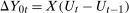 so that the unconditional distribution of
  depends on X, and hence, the Unconditional Difference in Differences Assumption does not hold.
 .
.
Appendix A: Proofs
A.1 Identification
A.1.1 Identification without covariates
In this section, we prove Theorem 1. Namely, we show that the counterfactual distribution of untreated potential outcomes,  , is identified. First, we state two well-known results without proof used below that come directly from Sklar's theorem.
Lemma A.1.For two continuously distributed random variables X and Y, their joint density in terms of the copula pdf is given by

Lemma A.2.For two continuously distributed random variables X and Y, their copula pdf in terms of their joint density is given by

Proof of Theorem 1.To minimize notation, let  be the joint pdf of the change in untreated potential outcomes and the initial untreated potential outcome for the treated group, and let
  be the joint pdf in the previous period. Similarly, let
  and
and  be the copula pdfs for the change in untreated potential outcomes and initial level of untreated outcomes for the treated group at period t and
  , respectively. And, finally, let
  (the support of the change in untreated potential outcomes for the treated group) and
  (the support of outcomes for the treated group in period
  ). Then
 (3)
(3) (4)
(4) (5)
(5) ) using Lemma A.2.
Now, make a change of variables:  and
and  . This implies the following:
- 1.
- 2.
- 3.
- 4.
 .
.
 and
and  cancel out the fractional terms in the third and fourth lines of Equation (5) implies
 (6)
(6) (7)
(7) (8)
(8)A.1.2 Identification with covariates
In this section, we prove Propositions 1 and 2.
Proof of Proposition 1.All of the results from the proof of Theorem 1 will still go through with the exception of the last step which uses the Unconditional Distributional Difference in Differences Assumption. Therefore, all that needs to be shown is that  under the conditions in Proposition 1. Notice
 (9)
(9) (10)
(10) (11)
(11) with
with  and then multiplying by
  which holds because the expectation conditions on
  . Additionally, conditioning on
  allows us to replace the potential outcome
  with the actual outcome
  because
  is the observed change in potential untreated outcomes for the untreated group. Finally, Equation (11) simply applies the law of iterated expectations to conclude the proof. □
A.2 Proofs of claims in Examples 1, 2, 3
A.2.1 Proof of the results in Example 1
For the first part, notice that  . This has the same distribution for the treated group and untreated group under Condition (i).


 and
and  . The fourth equality holds by Condition (ii).
A.2.2 Proof of the results in Example 2
We prove each claim in turn.
Unconditional mean difference in differences holds

 and the third equality holds because the marginal distribution of time varying unobservables does not change over time. This result implies that both for the treated group and untreated group the average change in untreated potential outcomes is 0 which implies the claim.
Conditional Distributional Difference in Differences holds

 .
.Unconditional Distributional Difference in Differences does not hold

 because the distribution of X can be different across the two groups.17
Unconditional Copula Stability holds

 follows the same distribution as
  . This implies that the Copula Stability Assumption holds.
A.2.3 Proof of the results in Example 3
We prove each claim in turn.
Unconditional mean difference in differences does not hold

 (though this step is not required for the claim here to hold). This makes it clear that the (unconditional) path of untreated potential outcomes for each group depends on the distribution of X which may not be the same across groups.
Note that this also implies that the Unconditional Distributional Difference in Differences Assumption does not, in general, hold either.
Conditional Distributional Difference in Differences holds

Note that this also implies that conditional mean DID holds in this example.
Conditional Copula Stability Assumption holds
This follows using identical arguments as for the Unconditional Copula Stability Assumption in Example 1 after conditioning each expression on X.
Unconditional Copula Stability Assumption does not hold
Here, we provide a simple counterexample. Suppose, for individuals in the treated group,  ,
,  for
for  ,
,  , and all random variables are mutually independent. Also, suppose that
  ,
,  , and
, and  . This setup implies that each outcome is normally distributed, the change in outcomes is normally distributed in all time periods, and the copula between the change in outcomes and the initial level of outcomes only depends on the correlation between the two. Here, it is straightforward to show that
  . Intuitively, in the first period, an individual's rank does not depend on X; in the second period, individuals with a large value of X tend to move toward the bottom of the distribution; and in the third period individuals with a large value of X tend to move toward the top of the distribution. This results in the copula changing over time. The intuition of this counterexample also extends to the general case—when the trend in untreated potential outcomes depends on X in an unrestricted way, the (unconditional) copula of the change in untreated potential outcomes and the initial level is likely to change over time.
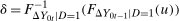
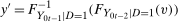
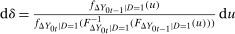
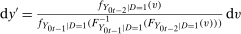
Appendix B: Asymptotic normality and inference
This appendix considers the asymptotic properties of our estimator of the QTT. We show that our estimator of the QTT converges uniformly to a Gaussian process. Our results essentially follow because empirical distribution functions converge uniformly to Gaussian processes and because we show the Hadamard differentiability of the map from distribution functions to the QTT. We also provide formal justification for using the empirical bootstrap to conduct inference as discussed in the main text. We provide similar results for the case where the Distributional Difference in Differences Assumption holds after conditioning on covariates in the Online Supplementary Appendix.
Before proving the main results, we state an additional assumption.
Assumption B.1.For  ,
,  and
and  is compact.

 and
and  . Next, let
  with support
  ; these are pseudo-observations if each distribution and quantile function were known. Let
  . Then define

As a first step, we establish a functional central limit theorem for the empirical processes of each of the terms used in our identification result. Let  denote the space of all uniformly bounded functions on the set S that are equipped with the supremum norm
  and let
  denote the space of all continuous functions on the set S.
Proposition 3.Under the Distributional Difference in Differences Assumption, Copula Stability Assumption, and Assumptions 3.2, 3.3 and B.1,

 where
where  is a tight Gaussian process with mean 0 and block diagonal covariance function
  where
where


 and
and  and where

Proof of Proposition 3.The result follows immediately from the functional central limit theorem for empirical distribution functions (see, e.g., van der Vaart and Wellner (1996)). □
Next, we work to establish the joint limiting distribution of observed treated outcomes and counterfactual untreated potential outcomes for the treated group. The key step in showing this result is to establish the Hadamard differentiability of the counterfactual distribution of untreated potential outcomes for the treated group. Before stating the main result, we provide several helpful lemmas.
Let  where
where  , for
, for  , are distribution functions; we assume that each
  has compact support
  . We also suppose that each
  has a density function
  that is uniformly bounded away from 0 and ∞ on its supports. Let
  be two random variables on
  with joint distribution
  . We assume that
  and that
  and that the conditional distribution
  has a continuous density function
  that is uniformly bounded from 0 and ∞.
 , let
, let


 and let
 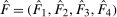 denote a vector of consistent estimators of
  .
.As a first step, we establish the Hadamard differentiability of  . We do this in several steps. First, we use the following result due to Callaway, Li, and Oka (2018).18
Lemma B.1.Let  and define the map
  as
as

 where
where  is the set of all distribution functions with strictly positive, bounded densities. Then, the map Ψ is Hadamard differentiable at
  tangentially to
  with derivative at
  in
in 

Lemma B.2.Let  . Define the map
  , given by

 . Then the map Λ is Hadamard differentiable at
  tangentially to
  with derivative in
  given by

Proof.Let  be given by
  . Lemma 3.9.25 of van der Vaart and Wellner (1996) implies that the map
  is Hadamard differentiable at Ξ tangentially to
  with derivative in
  given by

 be given by
  . Lemma 3.9.27 of van der Vaart and Wellner (1996) implies that
  is Hadamard differentiable at ϒ tangentially to
  with derivative at ϒ in
  given by


Lemma B.3.Let  . Define the map
  given by

 is Hadamard differentiable at
  tangentially to
  with derivative at
  in
in  given by

Proof.The proof follows by the same argument as in Lemma B.1. □
Lemma B.4.Let  and consider the map
  given by

 where
where  where
where  is the set of all distribution functions with strictly positive and bounded densities. Then the map ϕ is Hadamard differentiable at
  tangentially to
  with derivative in
  given by

Proof.First, notice that

 where
where  is the set of all functions
  for
for  as
as

 and
and  ,
,  .
.Using the same arguments as in Callaway, Li, and Oka (2018, Lemma A2), π is Hadamard differentiable tangentially to  with derivative at
  in
in  given by
 (12)
(12)
The following proposition is a main theoretical result of the paper and establishes the joint limiting distribution of the distribution of (observed) treated potential outcomes for the treated group and counterfactual untreated potential outcomes for the treated group.
Proposition 4.Let  and let
  . Under the Distributional Difference in Differences Assumption, Copula Stability Assumption, and Assumptions 3.2, 3.3 and B.1,

 and
and  are tight Gaussian processes with mean 0 with almost surely uniformly continuous paths on the space
  given by


Here,  is the variance that would obtain for estimating the counterfactual distribution of untreated potential outcomes for the treated group if each distribution and quantile function were known. The second term comes from having to estimate each of these distribution and quantile functions in a first step.
Proof of Proposition 4.First, notice that, uniformly in y,

With Proposition 4 in hand, our main result for the QTT follows straightforwardly by the Hadamard Differentiability of quantiles. We next state as a theorem the limiting process for our estimator of the QTT.
Theorem 2.Suppose  admits a positive continuous density
  on an interval
  containing an ε-enlargement of the set
  . Under the Distributional Difference in Differences Assumption, the Copula Stability Assumption, and Assumptions 3.2, 3.3 and B.1,

 is a stochastic process in the metric space
  with
with

Proof of Theorem 2.Under the conditions stated in Theorem 2, the result follows from the Hadamard differentiability of the quantile map (van der Vaart and Wellner (1996, Lemma 3.9.23(ii))) and by Proposition 4. □
Finally, for this section, we state a result on the validity of the empirical bootstrap for our procedure.
Theorem 3.Under the Distributional Difference in Differences Assumption, Copula Stability Assumption, and Assumptions 3.2, 3.3 and B.1,

 are as in Theorem 2 and
  indicates weak convergence in probability under the bootstrap law (Gine and Zinn (1990)).
Proof.The result holds because our estimate of the QTT is Donsker and by Theorem 3.6.1 in van der Vaart and Wellner (1996). □