Demographic transition, industrial policies, and Chinese economic growth
Abstract
We build a unified framework to quantitatively examine how demographic transition and industrial policies have contributed to China's economic growth in the past five decades. On the demographic side, we consider evolutions in government population-control policies, life expectancy, and pension income replacement. Industrial policies include changes in the speed of the growth of entrepreneurship, industry-specific interest subsidies, and financial intermediation costs. Our analyses suggest that the demographic transition alone hardly affects the aggregate savings rate, mainly due to general equilibrium feedback effects from prices. However, demographics account for a considerable fraction of the increase in per capita output growth since 1970. By comparison, industrial policy changes contribute significantly to the rise in both the aggregate savings rate and per capita output growth during the period. Notably, the interactions between the demographic transition and industrial policy changes cause aggregate savings to rise, but have little effect on per capita output growth. A novel factor of the model is endogenous human capital accumulation, a driver of per capita output growth. Our results are robust to the endogenization of fertility decisions.
1 Introduction
In this paper, we build a framework encompassing structural changes in demographics and industrial policies to study the evolution of the Chinese economy over the last five decades. The reasons are twofold. First, demographic changes, due mainly to the implementation of population control policies and the increase in life expectancy, and the implementation of various industrial policies, including privatization and preferential credit policies, constitute some of the most dramatic changes in Chinese society over the last several decades. And crucially, their implementations often overlapped.1 Second, there are strong reasons to believe that there are interactions between these two changes. For example, a direct implication of household aging is increased savings. Limited resources, however, force households to trade off between savings in financial assets and investing in their children's human capital, and thus, affect the quantity of capital and labor supplied to firms. Preferential credit policies affect both returns to physical capital and household savings. Thus, to gauge the relative importance of the structural changes and, more importantly, to arrive at the relevant policy implications requires a general equilibrium model of households and firms that accounts for these complex interactions. Our paper is the first to present such a framework and to demonstrate that both structural changes impacted per capita output growth significantly, and demographics alone do not drive aggregate savings but rather the general equilibrium feedback effects between the demographics and firm-side policy changes. As such, a paper that has only worker-side or firm-side changes is missing an important part of the story and can be misleading.
Specifically, we develop an overlapping-generations model where parents make human capital investment decisions for their school-age children, and grown children make transfer payments to their elderly parents. On the firm side, there are two intermediate goods sectors, one final goods sector, and one education sector. The two intermediate goods sectors differ in capital and labor intensity and their cost of capital due to government credit policies as in Chang, Chen, Waggoner, and Zha (2015). The labor-intensive industry allows for two types of firms, state-owned firms and private firms owned by entrepreneurs, as in Song, Storesletten, and Zilibotti (2011). In addition to differences in productivity, the state and private firms also differ in that the private firms face a borrowing constraint tied to their internal capital.2 Finally, we capture the financial market friction through intermediation costs. The government finances pensions through a payroll tax and finances credit market subsidies to firms through an income tax.
Using the calibrated model that matches important aspects of the Chinese economy, we show that declining fertility rates, lengthening life expectancy, and changes in the pension replacement rate during retirement have little bearing on the rise in total savings relative to output. The reason is as follows. For fixed interest rates and wages, these combined demographic factors lead households to save more and invest more in their children's human capital because they now need to provide for their longer retirement with smaller transfers coming from their children. Once the old generations retire and die off and the newborns enter the labor market, labor supply contracts, resulting in lower investment demand. In general equilibrium, the interest rate decreases, and the wage rises. These general equilibrium effects reduce incentives to save but increase incentives to invest in children's human capital as the present value of future transfers is higher with a lower interest rate and higher wage rate. In our exercise, the general equilibrium price feedback effects almost completely undo the positive impact of the demographic transition on savings. The demographic changes, however, account for 39% of the increase in per capita output growth since 1970.3
By contrast, the firm side developments, including changes in the speed of the growth of entrepreneurship, industry-specific interest subsidies, and financial intermediation costs, affect total savings rate and per capita output growth during the transition. The declining financial intermediation costs and initial interest subsidies to the capital-intensive industries encourage capital investment, driving up the capital-output ratio. Interest rates rise in response, and so do savings. These effects, combined with the movement of TFPs, cause per capita output to grow significantly in all but the last few years of our sample period when TFP growth turns negative in both sectors. Overall, firm-side changes account for almost 60% of the increase in per capita output growth between 1970 and 2019.
Importantly, we demonstrate that meaningful interactions exist between demographic and firm-side changes. These interactions contribute to an additional 4 percentage points or 12% in the raise of savings rate but have little impact on per capita output growth. Several forces drive these results. First are the price effects: Demographic factors and firm-side policies have conflicting impacts on interest rates and wages. The second driver, particularly concerning the large positive effects on savings, is the behavior of entrepreneurs who respond to both demographic and firm-side policy changes.
We conduct several counterfactual analyses to first show that the general equilibrium feedback effects are essential because significant price adjustment is both a feature of the data and the model. Additionally, endogenous human capital accumulation plays a critical role in our model, particularly in driving per capita output growth in the later periods of the sample. Finally, we present a version of the model where we endogenize the fertility decision following the classic approach that households also derive utility from having children.4 We calibrate these preference parameters to match the fertility rates in Taiwan during periods when Taiwan had per capita GDP growth similar to China's and demonstrate that the population control policy significantly reduced population growth. Without the population control policies, relative to the benchmark, the population would have been more significant, the labor supply would not have contracted, and the capital-output ratios would not have increased as much after 1995. Endogenizingly determined higher fertility also leads to less investment in human capital per child and eventually causes aggregate saving rates to exceed those of the benchmark after 1990. Per capita output, by contrast, grows more slowly than the benchmark before 2000 due to the larger population but then exceeds that of the benchmark as the economy begins to benefit from the additional labor supply. Between 1971 and 2019, GDP per capita growth would have been 0.34 percentage points lower without fertility control. In summary, although per capita growth initially benefited from the population control policy, the economy ultimately suffered from fewer workers as the birth-control policy reduced population, and thus, aggregate output by 61% in the long run.5
In terms of the literature, the findings that demographic changes alone do not account for the rise in savings echo Li, Zhang, and Zhang (2007),6 which demonstrate that longevity and the old-age dependency ratio drive aggregate savings in opposite directions in a growth model, and Banerjee, Meng, Porzio, and Qian (2023), which argue that general equilibrium forces can offset the negative correlation between household savings and fertility rate.7 Our findings are also consistent with the empirical findings in Baker, Benmelech, Zhang, and Yang (2022) that population control policies are not the primary causes of high levels of savings among Chinese households and with Chamon and Prasad (2010), who find that rising private expenditures on housing, education, and health care, as well as the lack of financial development rather than population control policies are the primary reasons for the high savings rate in China.8
Our firm-side analyses relate to the literature that seeks to explain the fast growth in China. The explanations explore the role of resource reallocation from agriculture to manufacturing and services (Brandt, Hsieh, and Zhu (2008), and papers cited therein), from state-owned enterprises to private enterprises (Brandt, Hsieh, and Zhu (2008), Hsieh and Klenow (2010), Song, Storesletten, and Zilibotti (2011), Song, Storesletten, and Zilibotti (2014), Chen and Irarrazabal (2015), and Liu, Spiegel, and Zhang (2021)), and from the capital-intensive sector to the labor-intensive sector (Chang et al. (2015)). We contribute to this literature by considering multiple policy changes and by incorporating the evolution in demographics on the household side.
Finally, our analysis is conducted in a general equilibrium framework with a balanced current account, that is, we implement strict capital controls. We believe it is important to model the real interest rate in China as endogenous because with the exception of the Great Recession when the Chinese government issued a rescue package worth over 4 trillion RMB, the current account balance as a share of total GDP remained under 4%, and Chinese financial markets were not fully integrated into world financial markets. Notably, the household saving and investment rates have generally tracked each other.
The rest of the paper is organized as follows. Section 2 presents the motivation and background of the paper. Section 3 describes the model. Section 4 calibrates the model and shows the transition dynamics between the two balanced growth paths. Section 5 conducts decomposition exercises to investigate the respective roles of household side and firm side changes. Section 6 studies the general equilibrium price feedback effects in economies with fertility policy and household side changes only. Section 7 analyzes the role of endogenous human capital accumulation. Section 8 endogenizes the fertility decision and discusses the role of the population-control policy. Section 9 concludes. The Supplemental Appendix, Dotsey, Li, and Yang (2025), contains the derivation of first-order conditions with households' fertility decision and the construction of fertility wedges as well as additional figures. The Supplemental Appendix will be referred to throughout the paper as SA.
2 Motivation and background
In this section, we draw on the existing literature and numerous data sources to document changes in the Chinese economy for the past five decades. We first illustrate the Chinese economy's rapid growth, then describe the aging of the Chinese population and the contributing factors behind this phenomenon. Lastly, we provide evidence of the evolution of industrial policies and credit market frictions and their consequences.
2.1 The rapid growth of the Chinese economy
The Chinese economy has grown rapidly over the last few decades (Figure 1). From 1970 to 1984, the per capita GDP growth went from 3% to over 10%. Then it hovered between 6% and 11% until 2019. The growth is even more astounding in relative terms. Before 1980, per capita GDP in China was only 1% of the U.S. By 2019, the ratio had shot up to over 17%.
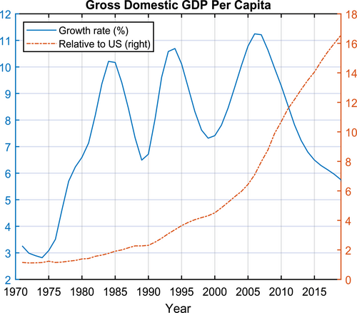
The Growing Chinese Economy. This figure depicts the Chinese economy's per capita GDP growth rate and per capita GDP relative to that in the U.S. Data source: World Bank/Haver Analytics. The per capita output growth series is HP-filtered.
2.2 The aging population
The aging Chinese population is best described by the declining young-age dependency ratio, the ratio of people under the age of 15 to people between the ages of 15 and 64, as well as the declining trend in the population growth rate. According to Figure 2a, the young-age dependency ratio was over 70% in 1970 but declined to under 30% in 2019. The population growth rate began to decline in the early 1970s and reached a trough of 1.3% in 1980. Though the growth rate recovered to its 1975 level in 1987, it subsequently began another long decline. By 2019, the growth rate had fallen to less than 0.3%.
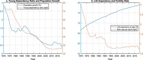
The Aging Chinese Demographics. This figure describes the population growth rate, young-age-dependency ratio (panel a), and life expectancy and fertility rate per adult (panel b). The young-age-dependency ratio is defined as the ratio of people younger than 15 to people between the ages of 15 and 64. The fertility rate per adult is half of the total fertility rate, the number of children that would be born to a woman if she were to live to the end of her childbearing years and give birth to children according to current age-specific fertility rates. Data source: World Bank and United Nations.
Two causes underly the aging of Chinese society. One is the reduced fertility rate and the other is the increase in life expectancy (Figure 2b). According to the World Bank, the fertility rate per adult9 fell drastically from 3 children per adult in 1970 to about 1.4 in 1980. After staying close to that level, the rate began to fall reaching 0.8 by 1995 and then remained below 1. The Chinese government started seriously promoting family planning in 1971 to curb population growth, with the propaganda: “One child isn't too few, two are just fine, and three are too many.” The tactics included initiatives that encouraged postponing marriage until a later age, lengthening birth spacing between children, and reducing the number of children, as summarized by the slogan: “Later, longer, and fewer.”10 In the late 1970s, the government adopted a stricter approach. It began imposing a limit on the number of children per couple: a two-child limit was implemented nationwide in 1978, followed by the one-child policy announced in 1979.11 In 2013, the Chinese government relaxed the one-child policy that had been in place since the late 1970s. Under the new policy, families could have two children if one parent, rather than both parents, was an only child. This policy, in practice, affected mostly urban couples. Starting in October 2015, the Chinese government completely abolished the one-child policy, and all Chinese couples are allowed to have two children. However, the policy barely increased fertility.12
Between 1970 and 2019, Chinese life expectancy improved markedly, from a low of 66 years of age for a person at age 23 in 1970 to a high of 79 years of age for the cohort at age 23 in 2019. For the life expectancy series, the year on the x-axis indicates cohort year, that is, the year when the individual turns 23.13
2.3 Industrial policies and credit market frictions
Since the late 1970s, the Chinese economy has experienced several major economic reforms. The continued reallocation of labor from agriculture to nonagricultural sectors occurred over late 1970s until the late 1990s. Additionally, the Chinese government actively encouraged private enterprises nationwide by introducing the first patent law, allowing state-owned enterprises (SOEs) to go bankrupt, and creating a more investor-friendly environment for private entrepreneurs. As a result, entrepreneurship went from nearly nonexistent to over 20% of the population between 1980 and 2019.14
During the last several decades, the Chinese government has also made considerable effort to improve the financial system. For example, the government deregulated the lending rate allowing for more competition and more flexibility in the pricing of loans. The increase in competition can be seen in the loan share of the four major state-owned banks, which fell from 61% in 1999 to 53% in 2004, and by the growing equity market (Podpiera (2006)). There is some evidence, documented in the papers that we cited above, that some of these subsidies may have peaked as the economy recovered from the global financial crisis, but it is not clear when these differential policies will be completely eliminated.
Furthermore, while Chinese government has always encouraged banks to favor state-owned enterprises, in the late 1990s, the government further deepened these credit policies, especially those targeting heavy industries. For example, Brandt and Zhu (2010) document that in 2007, more than half of all new capital formation went to the state sector. Bai, Lu, and Xu (2018) find that between 1997 and 2008, state-owned firms have higher leverage and pay much lower interest rates than nonstate-owned firms. Cong, Gao, Ponticelli, and Yang (2019) show that for manufacturing firms, the stimulus-driven credit expansion disproportionately favored state-owned firms and firms with a lower average product of capital, reversing the process of capital reallocation toward private firms that characterized China's high growth before 2008. Chen, Gao, Higgins, Waggoner, and Zha (2019) also find that bank credit in the 2000s, especially between 2009Q1 and 2010Q4, was disproportionally allocated to finance investment in real estate and other heavy industries populated with state-owned firms.15
3 The model
We consider an overlapping-generation model where intervivo transfers connect parents and children. Production takes place in industries that differ in capital intensity, productivity, and financial constraints. The government pays for its subsidies to firms and the pay-as-you-go social security system through taxation.
3.1 Firms
The economy consists of four sectors: two intermediate goods sectors, one final goods sector, and one education sector. The two intermediate goods sectors differ in productivity, capital intensity, and ownership structure. We term the sector that uses capital more intensively the capital-intensive or heavy-industry sector and the sector that uses labor more intensively the labor-intensive or light-industry sector. While the capital-intensive industry consists entirely of state-owned firms, the labor-intensive industry potentially contains both state-owned and private firms. This modeling choice thus combines the two approaches adopted in the literature on the Chinese economy as represented by Song, Storesletten, and Zilibotti (2011), Chang et al. (2015), and researchers cited in their papers. It also captures essential features of the Chinese economy: privately owned enterprises are concentrated in the labor-intensive sector; state-owned enterprises dominate the capital-intensive industry, and they benefit from subsidies from the government.
3.1.1 The final goods sector
3.1.2 The capital-intensive intermediate goods sector
3.1.3 The labor-intensive intermediate goods sector
The labor-intensive sector potentially consists of state-owned and privately owned enterprises. Compared with private firms, state-owned firms have better access to borrowing because of their close connection with state-owned banks. We assume that private enterprises have higher labor productivity, but are subject to borrowing constraints. Finally, we assume that goods produced by these two types of firms are perfect substitutes.
Problems of state-owned enterprises
Problems of private enterprises
3.1.4 The education sector
For simplicity, we assume a linear technology that transforms one unit of efficiency labor input into one unit of human capital investment. As such, units of human capital investment will cost the equivalent of units of final goods.
3.2 Households
In each period, a generation of individuals is born. Let B denote their birth year/cohort. The age of an individual of cohort B at time t is then . The individual starts working and forms a household upon turning age . The household gives birth to children at age , retires at age , and exits the economy after age , where . Following Song, Storesletten, and Zilibotti (2011), we assume that a fraction of the households are also endowed with entrepreneurial skills and use Λ to indicate whether a household is endowed with entrepreneurial skills.16
At each age, the household makes consumption and savings decisions. When children are between 7 and 22, the parent makes the human capital investment decisions for them. Labor supply is inelastic. Starting from retirement age, , the household also receives transfers from its children, at which point the children would be years of age, and we assume that to ensure that when the household retires, its children have already entered the economy. Finally, a retired household receives a social security pension, a fraction of its earnings for workers at the time of retirement, which is .
3.2.1 Labor income
3.2.2 Transfer payments to parents
3.2.3 Children's living expense
3.2.4 Human capital investment
Let denote the human capital of the child. We assume that the human capital accumulation function follows , where , and the parameter governs the child-age dependent efficiency in human capital production, and denotes the investment level in efficiency units of labor. This functional form is a slight modification of that used in Manuelli and Seshadri (2014). As noted before, units of human capital investment will cost the equivalent of units of final goods.
3.2.5 Income
A household receives labor earnings before retirement and a pension after retirement. Labor income is subject to a payroll tax with the revenue going toward the provision of pensions. Income is subject to an additional tax . The income structure differs for workers and entrepreneurs; we discuss them separately below.
Worker households
Entrepreneurial households
3.2.6 Recursive problems
Because we allow some parameters to vary by cohort and because wages, interest rates, and taxes vary over the transition path, households of the same age but from different cohorts solve different problems. To summarize, a household's state space consists of its cohort B, whether it is endowed with entrepreneurial skills, as indicated by Λ, age j, assets a, human capital h, and children's human capital .18 Table 1 describes a household's decisions at different ages.
|
Age |
[J1,Jf + 6] |
[Jf + 7,Jf + 15] |
[Jf + 16,Jf + 22] |
[Jf + 23,Jr,B − 1] |
[Jr,B,JB] |
|---|---|---|---|---|---|
|
Consumption |
yes |
yes |
yes |
yes |
yes |
|
Savings |
yes |
yes |
yes |
yes |
yes |
|
Children's human capital investment |
no |
mandatory |
optional |
no |
no |
|
Make transfer |
if |
||||
|
Receive transfer |
no |
no |
no |
no |
yes |
|
Receive pension |
no |
no |
no |
no |
yes |
- Note: This table describes decisions that a household makes at different ages. The symbol is the age at which the household enters the economy; is the fertility age; is the retirement age at which workers/entrepreneurs receive transfer from their children; and is the terminal age when the household exits the economy. Mandatory education is for children between the ages of 7 and 15. High school and college education between the ages of 16 and 22 is optional.
A household solves the following problem:
- 1. : the household either does not have children or has children under the age of 7 who do not require formal education yet;
The left-hand side of the budget constraint includes consumption, savings, basic living expenses for the children if the household is years of age or older, and the transfer the household makes to its parent when the parent is years of age or older and has not exited the economy yet.19 The right-hand side of the budget constraint contains the household's assets and after-tax income.
- 2. : the household has children who must receive mandatory primary and middle school education;
(27)Relative to households in the first age group, the family must now pay for its children's mandatory education, captured by in the budget constraint. In this case, the human capital investment decision is mandatory and is defined in equation (23). The law of motion for the children's human capital is represented by equation (27).
- 3. : the household has children who are eligible for optional high school and college education;
(28)(29)The household now makes human capital investment decisions for its children and the associated expenditure is captured by the fourth term in the budget constraint . The law of motion for the children's human capital is represented by equation (28).
- 4. : the household no longer has school-age children;
At this age group, as in age groups 1 and 2, the household makes only consumption and savings decisions. Its children have left the household and no longer cost anything. The household starts receiving transfer payments from the children after retirement, as captured by the last term on the right-hand side of the budget constraint.
3.3 The government
Finally, in each period, the government also specifies the fraction of entrepreneurs that can operate for each birth cohort B among households with entrepreneurial ability.
3.4 Equilibrium
Let denote total loans for private firms aggregated over all entrepreneurs. The competitive equilibrium consists of prices , government policies , allocations , , , and population measure such that, for given exogenous processes that govern the evolution of technology of all firms, intermediation cost, household life expectancy, fertility rate, retirement age and pension replacement rate:
- 1. Households maximize utility;
- 2. Firms maximize profits;
- 3.
Markets clear:
- (a) Goods market: all goods produced by firms are consumed by households or turned into investment;
- (b) Capital market: ;
- (c) Labor market: ;
- 4. The government balances the budget.
3.5 Balanced growth rates along the balanced growth path
Assuming that along the balanced growth path, the population grows at rate and labor augmenting technology at all firms grows at rate . The other economic variables will grow at rates specified in Table 2. Given that human capital investment is defined in terms of efficiency units of labor, in the balanced growth path, will remain constant. The growth rates of the other variables are straightforward.
|
Parameter |
Description |
Growth Rates |
|---|---|---|
|
Π |
Population measure |
gpop |
|
Y, Yk, Yl,Yl,i(i = s,p) |
Aggregate output |
(1 + gA)(1 + gpop)−1 |
|
K, Kk, Kl, Kl,i(i = s,p) |
Aggregate capital |
(1 + gA)(1 + gpop)−1 |
|
L, Lk, Ll, Ll,i(i = s,p) |
Aggregate labor |
gpop |
|
wt |
Per efficiency unit of wage |
gA |
|
cj, aj+1(j = J1,…,JB) |
Individual consumption and assets |
gA |
|
ih |
Endogenous human capital investment |
0 |
- Note: This table describes the growth rates for various variables at the balanced growth path.
4 Computation and calibration of the model
We assume the economy stays balanced until 1970 and calibrate our initial balanced growth path to be the average of the late 1960s. We assume a decline in the fertility rate beginning in 1971. Starting from 1979, we assume the rest of the exogenous changes became effective as a surprise. With the exogenous time-varying processes stabilizing, the economy converges to another final balanced growth path after 1000 years.20
To compute the transition path for a given sets of all the exogenous processes, we find the equilibrium path with a guess on the sequence of interest rates, wages, prices of the intermediate goods, and government income and social security taxes to compute the transition dynamics. Using this guess, we solve each cohort's consumption, saving, and human capital investment in children and solve the firm's problem each year. We search over the sequences of interest rates, wages, prices of intermediate goods, and government taxes until we reach a fixed point.
The model contains constant parameters and time-varying processes that we calibrate in two stages. In the first stage, we choose some parameters from the literature or the data. In the second stage, we jointly calibrate the remaining parameters and exogenous time-varying processes to match certain moments including time series along the transition path. We do so for fixed parameters because we have limited data for some earlier years, which makes identifying parameters from the initial balanced growth path alone infeasible.
4.1 First-stage calibration
The first-stage calibration choices are reported in Table 3.
|
Parameter |
Description |
Value |
Source |
|---|---|---|---|
|
Household |
|||
|
|
Initial age |
23 |
|
|
|
Fertility |
25 |
World Bank |
|
σ |
Relative risk aversion |
1 |
Macro literature |
|
|
Children living, required educ. exp. |
{0.040, 0.020} |
Chinese Household Income Project |
|
|
Transfer to parents |
{0.6500} |
|
|
Firms |
|||
|
|
Capital income share in k-sector |
0.54 |
Data, Chang et al. (2015) |
|
|
Capital income share in l-sector |
0.44 |
Data, Chang et al. (2015) |
|
φ |
Share of k-sector in final good prod. |
0.85 |
|
|
γ |
Elasticity of subst. bt. k- and l-goods |
2 |
|
|
δ |
Capital depre. rate in k- and l-sectors |
0.06 |
Standard |
|
gA |
Growth rate in balanced growth path |
2% |
|
4.1.1 Households
We assume that a household enters the economy at age 23 and gives birth to its children at age 25. We take a relative risk aversion parameter of 1 for preferences to make utility logarithmic. The parameters governing educational expenses, child living expenses, and transfers to parents mostly follow Choukhmane, Coeurdacier, and Jin (2023). In particular, we set the living cost of a child at 4% of a parent's labor income (). The mandatory education expense function is chosen so that it matches the labor income that urban households spend on their children's mandatory education by children's age (Figure 3 of Choukhmane, Coeurdacier, and Jin (2023)). As for parameters describing the transfer payments to parents we take from Choukhmane, Coeurdacier, and Jin (2023).
4.1.2 Firms
The capital income share of the capital-intensive and labor-intensive sectors, and , are calibrated to match the respective capital income and labor income shares of the two industries using data provided by Chang et al. (2015).21 We made a slight modification to this classification. Particularly, we reclassify the two industries with the highest labor income share in total output in the heavy sector, mining and transportation, into the light industry. This reclassification is to better capture corporate savings, which we assume is done entirely by private firms in the labor-intensive sector.22 The output share of capital-intensive sector in the final product and the elasticity of substitution between the capital-intensive and labor-intensive sectors are chosen according to Chang et al. (2015). The depreciation rate δ is set at a standard 6%. We choose the initial so that the GDP growth in our initial balanced growth path matches per capita GDP growth rate of 2% before 1970.
4.2 Second-stage calibration
The second-stage calibration includes a set of fixed parameters and time-varying processes that we chose to match selected economic moments and time series along the transition path.
4.2.1 Parameters fixed over time
For the household, these fixed parameters include the discount rate β, the labor efficiency profiles , parameter describing the transfer payments to parents the efficiency of human capital investment by children's age , and the weight on human capital investment in the human capital accumulation technology κ. On the firm's side, the parameters include the initial levels of labor augmenting technology in the capital-intensive sector and in the labor-intensive sector , as well as the parameter θ that governs the stringency of the collateral constraint for entrepreneurs. The will change during the transition as we introduce differential sectoral growth rates (see the detailed discussion in the following subsection). Still, we keep the ratio of constant as in the initial balance growth path.
The targeted moments include the age profile of earnings in 1986, the age profile of discretionary education expenditures in 2002,23 the deposit rate faced by households, the average relative capital-output ratio of state and private enterprises during the period of 1998–2005, and finally the loan to asset ratio for private firms as in Song, Storesletten, and Zilibotti (2011). We normalize the wage rate in 1970 to be 1.
We report parameters calibrated in the second stage in Table 4 and the target moments in Table 5. Note that because our overlapping generations framework abstracts from uncertainties in income and health expenditure, the model requires a discount factor that is close to 1 to be consistent with the observed savings rate.24 We set to 0.1482 so that kids transfer 10% of their labor income to elderly parents in the initial balanced growth path.
|
Parameter |
Description |
Value |
|---|---|---|
|
Household |
||
|
β |
Discount rate |
0.9966 |
|
|
Polynomial of human capital invest. efficiency |
[0.0030 −0.0590 0.2497 −1.5333] |
|
|
Transfer to parents |
0.1482 |
|
|
Polynomial of labor efficiency profile |
[9.3593e-06 −0.0028208 0.1857 −2.4763] |
|
κ |
Weight on human capital invest. |
0.45 |
|
Firms |
||
|
[, , ] |
Initial relative productivity |
[0.1468, 0.6083, 1.0231] |
|
θ |
Collateral constraint for entrepreneurs |
0.29 |
|
Moments |
Model |
Data |
|---|---|---|
|
Age profiles of earnings in 1986 |
Figure |
|
|
Education expenditure by age in 2002 |
Figure |
|
|
Capital-output ratio of state firms (1998–2005) |
2.06 |
2.65 (Song, Storesletten, and Zilibotti (2011)) |
|
Loan to asset ratio of private firms |
0.49 |
0.50 (Song, Storesletten, and Zilibotti (2011)) |
|
Average transfer to parents |
10% |
10% (Choukhmane, Coeurdacier, and Jin (2023)) |
|
Interest rate in 1970(%) |
5.50 |
5.00 (IMF) |
|
Wage rate in 1970 |
1 |
1 (normalization) |
To reduce the number of parameters, we estimate the efficiency function as a polynomial of degree of 3 concerning age, as is commonly done in the literature. In Figure 3, we depict the model-generated earnings profile in 1986 and the data counterpart.25 In terms of human capital investment, we estimate the efficiency function as a polynomial of degree of 3 and our estimate indicates that the efficiency and κ are identified by life-cycle education expenditure. We present the age-specific educational expenditure data versus model-generated moments in 2002 in Figure 4. The model matches both sets of data moments quite well.
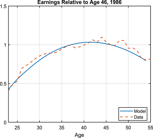
Age-Income Profiles. This figure depicts the labor earnings by age for Chinese households in 1986. Data source: Fang and Qiu (2023).
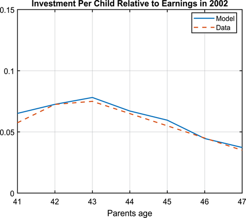
Optional Education Expenditure Profiles. This figure depicts optional education expenses per child as a fraction of parent earnings. The data come from Figure 3 in Choukhmane et al. (2023) (the green area that corresponds to discretionary education expenditure).
4.2.2 Exogenous processes
We now describe the calibration of the exogenous processes. To facilitate our discussion, we classify these processes into two groups: those that affect mainly households and those that affect mainly firms. On the household side, we have reductions in the fertility rate, increases in life expectancy, delays in retirement age, and changes in pension replacement rate. On the firm side, we have government policies that control the speed of the growth of entrepreneurship, and hence, the growth of private firms; credit policy that benefits capital-intensive heavy industry; the decline in intermediation cost; and time-varying labor augmenting technology.
Exogenous processes on the household side
In Figure 5, we chart the exogenous processes, including life expectancy at birth for a household of age 23 at the year plotted and birth rate per adult over time. Note that life expectancy in the model is discrete and can be increased only by integer numbers since the model period is one year. According to data from the World Bank, life expectancy at birth increased from 66 years for a person who was 23 in 1970 to 79 years for a person who was 23 in 2019. We assume that households expect to reach 80 years of age along the final balanced growth path.
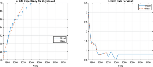
Exogenous Processes Along the Transition: Demographics. Life expectancy is defined as life expectancy at birth for a person at age 23 in the year plotted. Fertility rate is defined as the average number of births per adult. Data source: World Bank.
We chose the fertility rate to be 3 in the initial balanced growth path to match the population growth rate of 4.6% in the 1960s and set the fertility rate using data from the World Bank. We calculate the fertility rate as the fertility rate per adult, which is half of the total fertility rate. See Section 2.2 for the detailed discussion of the population control policies since 1970s. We target a long-run fertility rate of 0.8, the level currently observed in most developed countries.26 The implied growth rate of the population is −0.89% in the final balanced growth path.
In response to the aging population due to both the increase in life expectancy and the decline in fertility, the Chinese government implemented a policy to delay the retirement age. Since the 1950s, China has implemented a compulsory scheme to regulate the retirement age: 55 (60) for female (male) professionals such as teachers, medical personnel, other professionals, and administrators. For blue collar women, the retirement age is 50. In reality, however, many people take early retirement, as evidenced by the decline of cross-section income over the years starting at age 50. According to the Outline of the 14th Five-Year Plan (2021–2025) for National Economic and Social Development and the Long-Range Objectives Through the Year 2035, China will take small steps to raise the retirement age. To account for these developments, we set the retirement age for the initial balanced growth path at 55. We then began to raise the retirement age of a 23-year-old in 2001, by 1 year every 4 years. A 23-year-old from 2052 and onward will thus face a retirement age of 69, as seen in Figure 6.
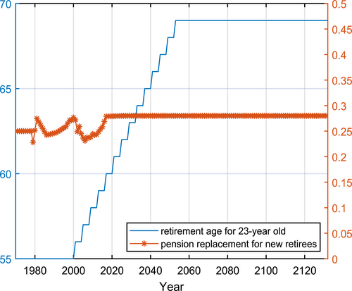
Exogenous Processes Along the Transition: Retirement. Pension replacement rate uses right y-axis. See the main text of the paper for data construction.
Around the same time, the government began reforming the pension system. The pre-1997 urban pension system was based on state and urban collective enterprises in a centrally planned economy. Retirees received pensions from their employers, with replacement rates as high as 80% in state-owned enterprises. The coverage, however, was low in private enterprises, especially in rural areas where the rate was 6%. The government has introduced many ambitious reforms since then. For example, the New Rural Resident Pension (NRP) was established in 2009 to cover rural residents, and the Urban Resident Pension (URP) was established in 2011 to cover urban nonemployed residents. The Social Insurance Law enacted in 2011 stipulated that rural migrant workers are entitled to the same treatment as urban workers. However, participation in these policies is voluntary, and compliance with the guidelines is poor.27 For our calibration, we take the replacement rate over the years for urban workers from Fang and Feng (2018) and keep the rural workers' pension replacement rate at 6%. We weigh the replacement rates for urban and rural workers by their respective population share (obtained from the China Statistics Year Books) and arrive at a time series of pension replacement rates for the general population, . Then the thus constructed rate exhibits a slight improvement over time (Figure 6).
Exogenous processes on the firm side
Figure 7 depicts the five exogenous processes on the firm side: the respective growth rates of labor-augmenting technology for the capital-intensive as well as the labor-intensive firms; the interest subsidy rate to the capital-intensive sector; the financial intermediation cost, and the fraction of entrepreneurs allowed to operate in each cohort of 23-year-olds in the economy. We assume that in the labor-intensive sector, labor-augmenting technology in the state-owned firms grows at the same rate as that in the privately owned firms. We chose these processes jointly to match five sets of moments: the overall capital-output ratio in the economy, the relative output as well as the relative capital in the capital-intensive sector to that in the economy, the changing employment share of private firms, and the fraction of the labor force that is self-employed. The aggregate capital-output ratios over time are constructed from the Penn World Table. The relative output and capital data are constructed using data from Chang et al. (2015) and from the China Statistical Yearbook of various years. The private employment share is constructed as follows. Using the China Statistical Yearbook Table 4-2 (“Number of Employed Persons at Year-end in Urban and Rural Areas”), we count individuals as working in private firms if they are self-employed or in nonstate-owned enterprises.28
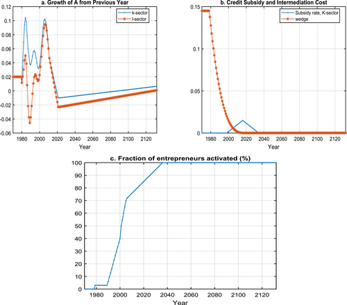
Firm Side Exogenous Processes Along the Transition. Panel a depicts the growth rates of labor augmenting technology for the K- and L-sector, respectively. On panel b, the solid line depicts exogenous government interest subsidy changes for firms in the K-sector along the transition path. The dotted line describes the intermediation cost. Panel c shows the fraction of entrepreneurs allowed to operate in each cohort of 23-year-olds.
The intermediation cost follows the logic of Song, Storesletten, and Zilibotti (2011) and captures operational costs, red tape, etc. In other words, this cost is an inverse measure of intermediation efficiency. We estimate the initial intermediation cost to be 14.5%. The intermediation cost is assumed to decline to zero in 2040, and the transition in the intermediation cost is linear after taking power transformation of 0.33.
Credit subsidies to capital-intensive firms were instituted in 2000, consistent with the narrative in Section 2.3. Although the large fiscal stimulus plan ended in 2010, the data show that the bank loan-to-GDP ratio remained elevated well into 2016 (Chen et al. (2019)). We assume that the subsidies to the capital-intensive firms peak in 2020 at 1.5 percentage points and decline to zero by 2038. For simplicity and to reduce parameter dimensions, we assume a linear transition path in the subsidy rate leading to the peak and returning to zero.
Figure 7c charts the fraction of entrepreneurs allowed to operate in each cohort of 23-year-olds in the economy, chosen by the government and directly governs the growth of private firms in the labor-intensive sector. Note that in our setup, as a departure from Song, Storesletten, and Zilibotti (2011), entrepreneurs receive an efficiency wage and a higher return on capital. As a result, entrepreneurs will continuously operate their businesses if allowed by the government. Our initial balanced growth path is an economy with no private enterprises. The fraction of entrepreneurs is thus set to zero. During the transition, the series is chosen to match the fraction of self-employed people in the data.29 Mechanically, we set 30% as the upper bound of entrepreneurship in the economy, a level slightly higher than currently seen in more developed Asian economies such as South Korea.30 We then adjust the fraction of households that can operate as entrepreneurs starting in 1990, along with other parameters, to roughly match self-employment in the economy without deviating too far from several other economic statistics along the transition path such as the private employment share.
In Figure 8, we chart model implications against data for targeted statistics on the firm's side: the ratio of output in the capital-intensive sector to total output, the ratio of capital input in the capital-intensive industry to total capital in the economy, private firms' employment share in overall employment, the overall capital-output ratio in the economy, and the fraction of the labor force that are self-employed. For the most part, the model reasonably fits the data. Since the 1990s, the capital-intensive heavy industry has become increasingly important in output and capital. Private firms have also become increasingly important. Their share of employment went from near zero in the early 1980s to over 60% by 2010.31 The economywide capital-output ratio has also been trending up during our sample period. Our model misses the fast rise in entrepreneurship in 1990 and the dramatic decline in the late 1990s in the data. That data trajectory, however, was entirely due to changes in self-employment in rural areas, with no consensus on the underlying driving forces.
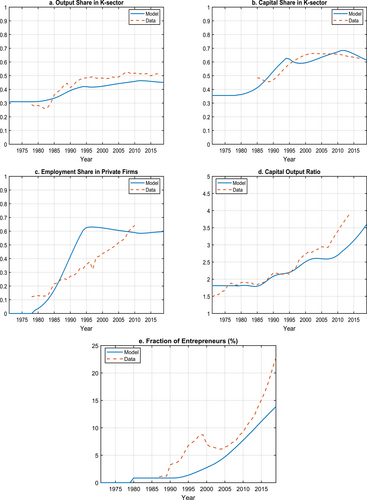
Firm Dynamics Along the Transition: Data versus Model. Data source: Panels a, b, and d: Chang et al. (2015) and China Statistical Yearbook; Panels c and e: China Statistical Yearbook and authors' calculation.
4.3 Nontargeted data moments versus model implied moments
We now describe the model's fit of some important data moments not used in parameterizing the model. How well the model accounts for these data represents a test of the model's capabilities.
4.3.1 Labor market outcome and return to human capital
To validate the modeling of endogenous human capital accumulation, we now evaluate the model's performance on various dimensions of human capital accumulation and the returns to human capital. One important empirical observation is that China's cross-sectional age-earning profiles have changed over time (Fang and Qiu (2023)). Our model matches age-earnings profiles from the household survey data reasonably well, as shown on the Figure 9a. Note that for each given year, the difference in wage earnings by age or cohort is a product of the life-cycle efficiency profile and the efficiency units from human capital investment. The life-cycle efficiency profile is constant over time.
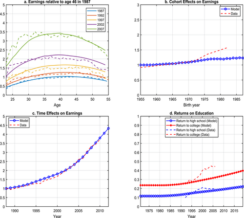
Return to Human Capital: Model versus Data. In panel a, earnings are from the Urban Household Survey constructed and provided to us by Fang and Qiu (2021). For panels b and c, the data come from Fang and Qiu (2021) Figure 4. The cohort effect is defined as intercohort human capital growth, and the time effect refers to changes in the human capital rental price, that is, wages over time. In panel d, the return to high school education in our model is defined for each individual as his human capital at age 19 over that at age 16. Similarly, return to college is defined as a person's human capital at age 23 over that at age 16. What is plotted is the log of the economywide average return to high school and college. The data come from Figure 1, panel b in Ge and Yang (2014).
To further decompose the forces that contribute to changes in cross-sectional age-earning profiles and isolate the effect of human capital investment on earnings, we next follow Fang and Qiu (2023) and construct the cohort effects as well as time effects on earnings and contrast them with their data counterparts (Fang and Qiu (2023) Figure 4) in Figures 9b and 9c. We define the cohort effect as intercohort human capital growth, reflecting human capital investment, and the time effect as changes in the price of human capital, which is the efficiency wage rate in our model. We normalize the first data points for both series, data, and model to 1. Our model captures the salient feature found in the data: the increase in the price of human capital (time effects) is more important than the increase in the quantity of human capital (cohort effects). In terms of fit, our model matches the time effects well but somewhat underpredicts the cohort effects, starting with the mid-1970s cohort.
One popular way to measure returns to human capital in the literature is to run a Mincerian regression, where wage is regressed on years of schooling. In China, a high school education takes 3 years, whereas a college education typically takes 4 years. In our model, as in Manuelli and Seshadri (2014), human capital investment is entirely on the intensive margin with years of investment fixed.32 There is no obvious mapping of human capital investment expenditure to years of schooling. We nevertheless conduct an analysis where we define, for each individual, the return to high school as his human capital at age 19 divided by his human capital at age 16, and the return to college as his human capital at age 23 divided by his human capital at age 16.33 We then take the average of these returns for each year to arrive at an economywide return to high school and return to college, respectively. We take the log of our measures of the returns to human capital and chart them against their data counterparts from Figure 1 in Ge and Yang (2014) in Figure 9d. Our model captures the data moments in the early 1990s but underestimates returns to college in later years. This is expected since our model does not feature any skill-biased technological change that is typically needed to explain these premiums.34
4.3.2 Capital market outcome
Section 4.2 showed that our model matches the sectoral capital allocation, output shares, and the aggregate capital-output ratio quite well (Figure 8). As an additional validation of our model, we chart in Figure 10 the dynamics of the return to capital net of depreciation. The model-implied marginal product of capital exhibits a downward trend, consistent with the data (Figure 7 in Bai, Lu, and Xu (2018) and Bai, Hsieh, and Qian (2006)).
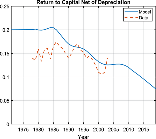
Marginal Product of Capital. Data come from Bai et al. (2006), Figure 7.
4.3.3 Growth and savings
We now turn to the two aggregate series of particular interest: aggregate savings as a ratio of total output and per capita output growth. Note that we follow Imrohoroglu and Zhao (2019) and treat savings by entrepreneurs as corporate savings.
Figure 11 graphs the two series. The model captures the increasing pattern of the aggregate national savings rate reasonably well. However, it overpredicts the saving rate for some of the periods, particularly after 2000. The model overpredicts household savings, and, as a result, it underpredicts the corporate saving rate.
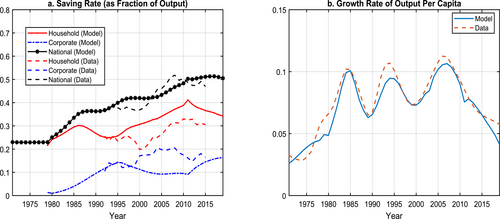
Savings Rate and Per Capita Output Growth: Model versus Data. Aggregate savings include household and corporate savings. Data on aggregate savings rate are provided by Chang et al. (2015). Data on per capita GDP growth are from the World Bank.
Turning to the growth rates of output per capita, the model generates growth substantially more significant than the assumed 2% exogenous growth rate in the initial balanced growth path due to the endogenous behavioral responses to changes in demographics and industrial policies. Average GDP per capita grows at the rate of 7.2% per year between 1971 and 2019, comparable to that of 7.6% in the data.
5 Decomposing contributions by firm- and household-side changes
Our model contains many structural features and important government policies. There are countless combinations of these policy changes, and we do not intend to isolate their effects here. Instead, we sort these changes into two groups: those that affect mainly firms and those that affect mainly households. On the firm side, we have government policies that control the speed of the growth of entrepreneurship, and hence, the growth of private firms; credit policy that benefits the capital-intensive heavy industry sector; time-varying technology growth; and the decline in intermediation cost, which helps all firms. On the household side, we have reductions in the fertility rate, increases in life expectancy, delays in retirement age, and changes in pensions. We conduct two counterfactual experiments, one where we implement changes we classify as the firm side only and the other where we implement changes we classify as the household side only. We are fully aware that many of the changes, for example, the reduction in intermediation costs, affect both households and firms directly, and all of the changes affect households and firms indirectly. We will highlight the interaction of firm structure and policy changes with demographic transitions on the various saving rates in our model and with the per capita output growth in Section 5.3.
5.1 The effects of firm structure and policy changes
To ascertain the combined contributions that the many firm-side changes have on the behavior of the economy, we consider an economy that experienced only the firm-side policy changes, mentioned above. Therefore, we keep all the household parameters, including the fertility rate, the same as in the initial steady state.
At a theoretical level, relative to the initial balanced growth path, the reduction in intermediation cost increases the effective return on savings for households and, as a result, will increase their incentive to save in physical assets and crowd out their investment in their children's human capital. The growth of entrepreneurs, who have higher returns to savings and thus higher saving rates than workers, also contributes to the saving rate increase. For output, the rise in physical assets leads to higher output growth. Reducing human capital investment, however, will lower labor efficiency and reduce output growth. Balancing this effect is the increase of entrepreneurial households, which increases total output as private firms are more productive than state-owned firms.
We chart the various economic statistics in this counterfactual economy and their benchmark counterparts in Figure 12. The dynamics of the counterfactual economy directly measure the effects of firm structure and policy changes. Their differences with the benchmark counterparts reflect the impact of demographic changes and their interactions with firm structure and policy changes.
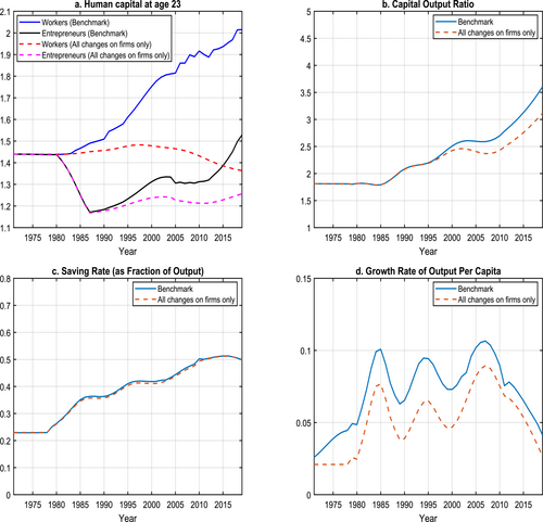
Selected Economic Statistics: Benchmark versus Firm-side Policy Changes Only Experiment. In the experiment, we implement only firm side structure and policy changes as detailed in Section 5.1. The solid lines depict the benchmark economy and the dashed lines depict the experiment.
In the counterfactual economy, displayed by the dashed lines in Figure 12, reductions in intermediation cost together with government preferential credit policy lead to higher returns to savings. Investments in children's human capital increase only very slightly, and the stock of human capital stays nearly flat for workers and declines for entrepreneurs who have strong incentives to save (and invest in their firms) instead. For the economy as a whole, the capital-output ratio goes up, rates of return to capital net of depreciation decline but wages increase. Relative to the initial balanced growth path, aggregate savings rise significantly. Output per capita grows steadily contributing to almost 60% of the per capita output growth rises since 1970.
Relative to the benchmark, the alternative economy has almost the same aggregate savings rate, driven by lower household savings. The counterfactual growth in output per capita is, however, significantly lower due to a lower physical capital stock and a lower human capital stock relative to the baseline. These differences demonstrate the importance of the effects of demographic factors and their possible interaction with firm structure and policy changes, which we investigate next.
5.2 The effects of demographic changes
Turning to the contributions that all the demographic factors have on the economy's behavior, we investigate an economy that experienced only the demographic changes, including increases in life expectancy, population control policies, changes in pensions, and an increase in the retirement age.
Intuitively, relative to the initial balanced growth path in 1970, the lower fertility rate and the lengthened life expectancy should push households to save more and invest in their children's human capital. Endogenously increased human capital investment causes savings to go down but increases effective labor supply. As the population gets older, however, labor supply contracts. Delaying the retirement age reduces savings, increases labor, and discourages households from investing in their children's human capital. The increase in the pension replacement rates is relatively minor, and we expect households' savings to decline slightly in response. Relative to the benchmark economy, no private firms mean no corporate savings; thus, national savings equal household savings. Without entrepreneurs, firms in the labor-intensive sector are less productive than in the benchmark.
We report the various economic statistics in this alternative economy along with their respective benchmark dynamics in Figure 13. To reiterate, the dynamics of the alternative economy directly measure the effects of the demographic transition that starts in 1971, and their differences with the benchmark reflect the effects of the missing firm structure and policy changes, and their interactions with demographic transitions.
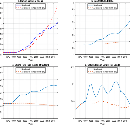
Selected Economic Statistics: Benchmark versus Household-side Policy Changes Only Experiment. In the experiment, we implement only demographic transitions as detailed in Section 5.2. The solid lines depict the benchmark economy and the dashed lines depict the experiment.
In response to the demographic changes, households immediately increase their investment in their children's human capital. Workers' human capital at age 23, thus, rises significantly starting in the mid-1990s when the children born in 1971 or after enter the labor force. Households also begin to save more relative to the initial steady state, leading to slow increases in the capital-output ratio. On net, total savings as a fraction of output are nearly flat. Per capita output growth takes off immediately. Demographic changes account for 39% of the increase in per capita output growth since 1971.
In contrast to the benchmark, the counterfactual economy experiences higher human capital for workers at age 23 after 2005 but a much lower capital-output ratio. Aggregate savings rates are much lower than those in the benchmark economy; per capita output also grows much more slowly, partly reflecting the absence of private entrepreneurs. These differences point to the significance of the effects associated with firm-side structure and policy changes and their possible interactions with the demographic transition.
5.3 The interaction of firm structure and policy changes with demographic changes
In this subsection, we highlight the interaction of firm structure and policy changes with demographic transitions on our model's saving rates and per capita output growth. The interaction effects arise from the general equilibrium effects coming from wages and interest rates and from entrepreneurs being directly affected by both policy changes.
We obtain numerical estimates of the interaction effects by combining the analysis in the preceding two subsections. Specifically, three sources drive the dynamics of the benchmark economy: firm-side changes, household-side changes, and the interaction of both changes. Therefore, subtracting the results in the household-side changes in Section 5.2 from the benchmark results gives the effects from firm-side changes plus the interaction term (the solid lines in Figures 14a and 14b). We then take out the values in the initial balance growth path from the firm-side changes found in Section 5.1 and obtain the effect of firm side changes without the interaction term (the dashed lines in Figures 14a and 14b). Next, we remove the dashed lines from the solid lines and arrive at the effects of the interaction term, displayed in Figures 14c and 14d.35
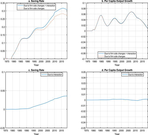
Savings Rate and Per Capita Output Growth: Impact of the Interactions of Firm Structure and Policy Changes with Demographic Transitions. The solid lines in panels a and b are results from Section 5.2 subtracted from results from the benchmark, which capture effects due to the firm-side changes and their interactions with the demographic transitions. The dashed lines in panels a and b are results from Section 5.1 subtracted by their respective 1970 balanced growth path, which capture effects due to firm-side changes only. The lines in panels c and d are the difference between the solid lines and the dashed lines and capture the interaction. See Section 5.3 for more details.
Figure 14c shows that the interaction term contributes over 4 percentage points to the raise in aggregate saving rate between 1970 and 2019. Several forces drive these results. First are the price effects: Demographic factors and firm-side policies have conflicting impacts on interest rates and wages. The second driver, particularly concerning the large positive effects on savings, is the behavior of entrepreneurs who respond to both demographic and firm-side policy changes. Regarding per capita output growth, Figure 14d indicates that for much of the sample, the interaction term has little effect. These results stem from several factors. First, demographic and firm-side policies have conflicting impacts on interest rates and wages. Second, particularly for the positive effects on savings, entrepreneurs respond to demographic and firm-side policy changes, such as increases in entrepreneurship, and they increase savings significantly.
6 Understanding the demographic effects: Partial versus general equilibrium
Our Section 5.2 results demonstrate that demographic changes alone do not impact aggregate savings much. To show that these results are mainly driven by general equilibrium price feedback effects, in this section, we conduct two counterfactual analyses where we implement either population-control policies or all household-side changes only (discussed in Section 5.2) and contrast the results in the partial equilibrium setting with those in the general equilibrium setting.
We start with the exercise where we contrast the partial and general equilibrium results with only fertility changes and present the results in SA Figure A1. In partial equilibrium, with population controls, labor supply declines, though with a lag as individuals enter the labor force at age 23. Households respond to the reduction in fertility by saving more (panel e). They also invest more in their children's human capital to raise efficiency units of labor supply (panel b). These partial equilibrium effects on savings are consistent with the partial equilibrium analyses in, among others, Curtis, Lugauer, and Mark (2015) and Choukhmane, Coeurdacier, and Jin (2023). In general equilibrium, however, interest rates decline (panel a) to close the gap of increased capital supply from households and reduced capital demand due to shrinking labor supply (panel c), which reduces savings and overturns the negative correlation between household savings and fertility rate in partial equilibrium, echoing findings in Banerjee et al. (2023). As a result, wages increase more than in partial equilibrium (panel d), as do investments in human capital and the associated human capital stock at age 23 (panel b). The resulting higher efficiency labor supply more than offsets the decline in the saving rate, leading to faster output growth in the general equilibrium (panel f).
We repeat the exercise with household-side demographic changes. Among the household side changes, the increase in life expectancy positively affects savings and human capital investment, similar to the population-control policy. By contrast, the delay in retirement age, by reducing years in retirement and years receiving transfers from kids, has the opposite effect on aggregate savings and human capital investment. We expect the changes in replacement rate to have little impact on aggregate savings as the changes were insignificant. We present the results in SA Figure A2. In partial equilibrium, savings and investment in human capital move in the exact same directions and more significantly as in the previous exercise (panels b and e). In general equilibrium, however, interest rate declines and wage rises primarily offset the savings incentives. Hence, aggregate savings increase little relative to output. Adding all demographic changes leads to more substantial growth than the population controls—only experiments shown in SA Figure A1. In both exercises, the general equilibrium effects on per capita GDP growth are more favorable than the partial equilibrium effects.
7 The role of endogenous human capital accumulation
One unique feature of our model is the joint modeling of physical and human capital accumulation. Households rely on transfers from their children and savings to supplement their government pension in retirement. Transfers from children increase with the number of children and children's labor earnings. At the same time, the return on savings is governed by the return to capital net of intermediation costs for worker households and by the return to capital in their project for entrepreneur households. For a given amount of resources, families face a trade-off between investing in their children's human capital and saving on their own.
To quantitatively examine the importance of this interaction between human capital investment and savings, we conduct an experiment where we do not allow households to invest in human capital endogenously. Instead, we fix their human capital investment per child relative to income by age at the same ratio as in the initial balanced growth path. Although no private firms are allowed in the initial balanced growth path, we can still compute human capital investment per child relative to income by age for entrepreneurs. In our setup, entrepreneurs have access to higher returns to capital, implying that their incentive to save (and invest in their projects) is stronger than workers. As a result, entrepreneurial parents will always invest less intensively in their children's human capital than worker parents. We thus expect this counterfactual to have a more considerable impact on workers' behavior than on entrepreneurs.
We first chart the resulting human capital investment relative to earnings for workers and entrepreneurs for 2002 in SA Figure A3a. As expected, the rates fixed at the initial balanced growth path are much lower than in the benchmark for all the ages at which parents are eligible to invest voluntarily in their children's human capital. In SA Figure A3b, we plot each individual's human capital at age 23. Since we fix their human capital investment per child relative to income by age at the same ratio as in the initial balanced growth path, human capital for worker individuals barely changes over time.36
In this new economy, relative to the benchmark, given that parents are restricted in their ability to increase their old-age support through investment in their children's human capital, they will respond by saving more. On the labor side, lower human capital investment means lower labor efficiencies, which in turn implies lower household earnings and lower total output. In general equilibrium, however, interest rates fall in response, and wages rise, lowering the incentive to save. Note that human capital investment takes time, and human capital is a stock variable. It takes a whole cycle, a minimum of 32 years (55 − 23) to be precise, for the entire working-age population to have benefited from the endogenous accumulation of human capital. Therefore, its full impact on output growth materializes much later than on savings.
We present our simulation results for the new economy together with those for the benchmark economy in SA Figures A3, and for the remainder of the discussion, we will focus on the comparison with the benchmark economy. As shown in SA Figure A3c, with less human capital investment, there is more capital in the economy relative to output starting in 2000.37 Despite increases in the wage rate, lower labor efficiency leads to lower earnings relative to the benchmark, particularly in later years, as seen in SA Figure A3d. The aggregate savings rate declines slightly on the net (SA Figure A3e). Per capita output grows more slowly, particularly near the end of our sample, as shown in SA Figure A3f. In 2019, the per capita GDP growth rate was 0.85 percentage points higher with endogenous human capital accumulation.38
8 Endogenous fertility decision and the role of the population-control policies
Our baseline model, where we take fertility as given, is close to the reality of Chinese households: the population-control policy was in place for almost the entire data period and it was binding. In this section, we endogenize the households' fertility decisions. Then, using Taiwan's fertility rates at similar levels of per capita GDP as a proxy for the optimal fertility rate in China, we examine what would have happened in the absence of the birth-control policy.
8.1 Endogenizing households' fertility decisions
We augment our benchmark model with endogenous fertility decisions featuring quantity-quality trade-offs with old-age support, an essential motive for having children in developing countries such as China. As such, the model relates to an extensive literature, starting with Barro and Becker (1989) and Becker, Murphy, and Tamura (1990) but moving more closely toward the modeling strategy favored by Choukhmane, Coeurdacier, and Jin (2023). The crucial differences between our model and that of Choukhmane, Coeurdacier, and Jin (2023) are that our model is an endogenous growth model with rich firm dynamics and a general equilibrium model where we capture price feedback effects.
The households' problem remains the same as before, with two exceptions. First, the period utility now has an additional term from having children. Second, an additional constraint stems from the birth-control policies. It is immediately apparent that endogenizing the fertility decision does not change anything when the birth-control policy binds as in most of our baseline analyses. When the birth-control policy no longer binds, households make their fertility decisions, trading off the benefits of having children, which include the utility gain and future expected transfer payment and the cost of raising and educating children. SA A.1 presents the household's problem at age when it decides the number of children to have. The firm side of the economy remains the same as the benchmark.
8.2 The role of the population-control policies
To quantitatively investigate the role of population-control policies, we need to back out the cohort-specific preference parameters for having children. Our strategy here is to calibrate these parameters to match the fertility path of Taiwan, which experienced a similar economic growth path.40 Specifically, according to the World Bank data, Chinese per capita output growth occurs later than Taiwan's by about two decades. As such, we view the fertility rates in Taiwan since 1950 as the fertility rates China would have had since 1971 had it not been for the birth-control policies. According to SA Figure A5a, the thus constructed optimal fertility rates lie on top of the actual Chinese fertility rates until 2014.41 We then assume both economies have the same long-run fertility rate and set further fertility paths accordingly. In other words, the only difference between the two economies is the fertility path in the short run. After the two economies converge to the new balanced growth path, the per capita variables should be the same in the two economies.
Using the calibrated preference parameters for having children and keeping all policies intact except for the birth-control policy, we resolve the model and present our simulation results in SA Figure A5b to SA Figure A5f. With the now higher endogenous fertility rates, not surprisingly, human capital investment per child is much lower (panel b) as households spread human capital over more children. The capital-output ratio is also lower after the mid-1990s (panel c). As households' incentives to save decline and labor force rises, interest rates rise, and wages decline. The combined effect of lower labor efficiency and wage rates is lower earnings (panel d). Aggregate savings, shown in panel e, do not change much relative to the baseline initially but become larger after 1995, a direct result of more labor force in the economy (and hence, more capital demand in a growth model). Likewise, per capita output, shown in panel f, grows more slowly than the baseline but catches up in the early 2000s as the economy benefits from abundant workers. Between 1971 and 2019, GDP per capita growth would have been almost 0.34 percentage points lower without fertility control.
To summarize, the population-control policies alone did not increase the aggregate savings rate in the short to medium run. They even led to fewer savings relative to output. The reason is that a smaller population requires less capital in a growth model. Although per capita growth initially benefited from the birth-control policy, the economy ultimately suffers from less workers because the birth-control policy reduced population, and thus, aggregate output by 60% in the long run.
9 Conclusions
In this paper, we build a unified framework that brings together important changes on the household and firm sides of the Chinese economy to account for its rapid growth and elevated saving rate. On the household side, we focus on the demographic transition arising from the one-child policy, increased life expectancy, government policies that changed the pension replacement rate, and the delayed retirement age. On the firm side, we analyze government policies that have controlled the growth of private firms, credit policies that have favored different industries, financial development, and sectoral TFP changes over time. Our model also features endogenous human capital investment, a prominent part of the Chinese growth experience.
Our model does a reasonable job of accounting for the time trend of the aggregate saving rate and the growth rate of per capita output. Our analysis indicates that firm-side structure and policy changes were essential in driving China's high savings and rapid growth rate. Demographic changes, by contrast, did not affect aggregate savings but impacted growth later in the transition. Notably, the interaction of the two changes significantly impacted the aggregate savings rate but mutedly impacted per capita GDP growth. The paper thus links important insights from the literature that explains the fast growth in China and from the literature that focuses on the high saving rate and shows that there are important reasons to consider these various avenues in tandem. It is important to note that our paper abstracts from a potentially important consideration: stochastic mortality risk. Given the complexity of our model and, more importantly, the lack of micro data on Chinese family structures,42 we leave this to future research.


