We thank Matias Cattaneo, David Harris, seminar participants at Princeton University, Toulouse School of Economics, University of Auckland, University of Cambridge, University of Essex, University of Exeter, University of Melbourne, University of Surrey, University of Sydney, University of York, Universitat Pompeu Fabra, and conference participants at the 10th Italian Congress of Econometrics and Empirical Economics (University of Cagliari, 2023), the 5th International Workshop in Financial Econometrics (Bahia, 2023) and the Barcelona Workshop in Financial Econometrics (Universitat Pompeu Fabra, 2024) for comments. We gratefully acknowledge support from the Independent Research Fund Denmark (DFF Grant 10.46540/3099-00076B). Cavaliere and Rahbek also acknowledge support from the Italian Ministry of University and Research (PRIN 2020 Grant 2020B2AKFW).

About

Sections

PDF

Tools

Share a link

Email
Wechat
Bluesky

Abstract

Based on the GARCH literature, Engle and Russell (1998) established consistency and asymptotic normality of the QMLE for the autoregressive conditional duration (ACD) model, assuming strict stationarity and ergodicity of the durations. Using novel arguments based on renewal process theory, we show that their results hold under the stronger requirement that durations have finite expectation. However, we demonstrate that this is not always the case under the assumption of stationary and ergodic durations. Specifically, we provide a counterexample where the MLE is asymptotically mixed normal and converges at a rate significantly slower than usual. The main difference between ACD and GARCH asymptotics is that the former must account for the number of durations in a given time span being random. As a by-product, we present a new lemma which can be applied to analyze asymptotic properties of extremum estimators when the number of observations is random.

1 Introduction

In the seminal paper by Engle and Russell ( 1998 , ER henceforth), autoregressive conditional duration (ACD) models were introduced for modeling inter-arrival times, or durations, between financial transactions. Given some observation period

with

observed event times

, the durations

are given by

and modeled as

(1)

(2)

where the innovations

are strictly positive, i.i.d., and have unit mean,

The quasi maximum likelihood estimator (QMLE) of

is defined as

, with

the exponential likelihood

(3)

with initial values

and

. The true parameter value is denoted by

ER noted that the likelihood function in ( 3 ) is identical to the likelihood function of the GARCH(1,1) model with Gaussian innovations. In line with this, for their main result (p. 1135), ER referred to Lee and Hansen ( 1994 , LH henceforth) to conclude that under the condition of strict stationarity and ergodicity of the durations , that is, , is consistent and asymptotically normal at the usual rate.

As we argue in this paper, the machinery in LH cannot be applied to the ACD setup unless additional arguments are used and further assumptions imposed. In particular, with such that the strict stationarity and ergodicity condition holds, that is, , we argue that, in contrast to the GARCH case, the behavior of the QML estimator depends on whether (i) , (ii) , or (iii) . Specifically, results regarding rates of convergence, asymptotics of the QMLE, convergence of the score, and sample information all depend on which of the three cases above holds. Key is that modifications of arguments are needed due to randomness of the number of durations .

To preview why, consider the score and information, evaluated at the true value

(4)

(5)

To establish asymptotic normality of

, standard theory usually requires that these satisfy a central limit theorem (CLT) and a law of large numbers (LLN), respectively. The ACD setting, however, is not standard as the number of observations

is random, and not independent of the sequences

and

Note in this respect that the CLT and the LLN for deterministic number n of observations, that is (with N denoting the Gaussian distribution)

(6)

(7)

are not sufficient for their random

-analogues in ( 4 )–( 5 ) to hold. That is, it does not follow from ( 6 ) that

is asymptotically Gaussian even if

; see, for example, Chapter 1.3 in Gut ( 2009 ). Likewise, it does not follow that

is asymptotically Gaussian for some increasing deterministic sequence

. Hence, the arguments based on LH, which are based on

deterministic, do not apply.

This paper makes the following contributions.

First, we provide a new lemma which can be applied to analyze asymptotic properties of extremum estimators when the number of observations is random. The arguments in its proof use renewal theory and are thus different from LH/ER.

Second, we apply this result and show in Section 2 that under the additional condition , which implies , and T are proportional in the sense that . The latter result can be used to prove that normalizing the score by either , , or the sample information, , leads to asymptotic normality, establishing asymptotic normality of , , and ; see Theorem 2 .

Third, to illustrate that these results do not hold in general, we present in Section 3 a counterexample, with stationary and ergodic, but where , and hence . With exponential innovations , we show that converges at the rate for some , which is significantly slower than the usual rate. Moreover, has a mixed normal (MN) limiting distribution. Hence, the limiting distribution of the MLE differs from the classical, LH/ER form . Importantly, the MN limit theory implies that different normalizations lead to distinct asymptotic distributions.

Finally, we note that the arguments in the counterexample are specific to the MLE, and hence there is no guarantee that they can be generalized to the QMLE for the case of , and neither to the ‘unit root’ case of .

2 Main Result

In this section, we show that the asymptotic normality of the QMLE can be obtained by imposing the additional condition

, which implies

. The key insight is that if

, the random number of durations

over the observation period

satisfies

(8)

This in turn (as

) is sufficient for the deterministic n LLN in ( 7 ) to imply that its random

-analogue holds. To establish the random

-CLT for

in ( 4 ), the deterministic n-CLT in ( 6 ) is replaced by its stronger functional version

where B is a standard multivariate Brownian motion and convergence is on the space of càdlàg functions on

equipped with the

-topology.

To derive the asymptotic distribution of the QMLE presented in Theorem 2 , we make use of the following general lemma which extends the results in LH to allow for a random number of observations.

Lemma 1.Let be a random function of the parameter , indexed by . Assume that is three times continuously differentiable, and that for in the interior of Φ, as :

(C.1) , ,
(C.2) ,
(C.3) ,

where is a k-dimensional Brownian motion, is a closed neighborhood of , and . Moreover, with a counting process defined on the same probability space as , assume that for some constant :

(C.4) as .

With , there exists an open neighborhood , such that, as :

(i) With probability tending to 1, there exists a unique maximum point of in , is concave on , and ;
(ii) ;
(iii) , .

All proofs of the results in this paper are provided in Section 4 . Note that Assumption (C.4) can be replaced by and , .

Our main result is as follows.

Theorem 2.For the ACD model ( 1 )–( 2 ) with true parameter , assume:

(i) is an i.i.d. sequence of random variables with support , pdf bounded away from zero on compact subsets of , , and ,
(ii) is an interior point satisfying .

As , the maximizer of in ( 3 ) is consistent and asymptotically normal:

where

. Here,

, and

are given by ( 6 ) and ( 7 ), respectively.

Remark 1.Theorem 2 shows that, if the strict stationarity condition is strengthened with the additional restriction , then is asymptotically normal as . In particular, . In this case, using as normalization instead, Theorem 2 and ( 8 ) jointly imply that . Hence, up to a scaling factor, and have the same asymptotic distribution. Likewise, when normalizing by the sample information, we find for the MLE as then .

Remark 2.The proof of Theorem 2 relies on the new Lemma 1 , which may also be used to establish asymptotic theory for the more general ACD() models mentioned in ER (p. 1133) which allow lags of and lags of in ( 2 ), including the simple stylized ACD model considered in Cavaliere, Mikosch, Rahbek, and Vilandt ( 2024 ).

Remark 3.Asymptotic normality of the estimator is not guaranteed to hold when Assumption (ii) does not hold; see Section 3 for a counterexample.

3 Non-Standard Asymptotics

We present here a counterexample which shows that if , implying , the asymptotic distribution of is not normal, even under strict stationarity and ergodicity. Specifically, different normalizations (e.g., using a deterministic function of T, or a random normalization such as the sample information) may lead to different asymptotics.

Consider the ACD model given by ( 1 )–( 2 ), under the assumption that the 's are exponentially distributed with . We have the following result.

Theorem 3.Consider the exponential ACD model with true parameter being an interior point satisfying the strict stationarity condition and . As , the maximizer of in ( 3 ) is consistent and asymptotically mixed normal:

(9)

where

. Here,

is the unique solution of the equation

is defined in ( 7 ), and the random variable

is given in Lemma 4 .

The proof of Theorem 3 makes use of the key result that, when

(10)

rather than in probability to a positive constant; see Lemma 4 . Note that

is the (right) tail index of the durations; see ( 16 ) below. The convergence in distribution in ( 10 ) is non-standard and, importantly, implies the need for a different approach to show convergence results for sums of the form

; see, in particular, Section 4 .

In line with Remark 1 , the following corollary for normalized by the sample information or by holds.

Corollary 1.Under the assumptions of Theorem 3 , and as .

Remark 4.Consider a drifting sequence of true parameters of the form (). Using the same arguments as in the proof of Theorem 3 , it holds that , which is mixed normal with (deterministic) non-centrality parameter −s. In contrast, for normalized by the sample information as in Corollary 1 , we find , where the non-centrality parameter is now random. The latter result implies that when , the asymptotic local power of t-ratios is random in the limit, which contrasts with the case in Theorem 2 .

To shed some light on the mixed normality in Theorem 3 , note that when , the limiting distribution of does not have exponential tails; in particular, it has infinite variance. To see this, write the right-hand side of ( 9 ) as with standard normal, independent of , and let for any vector norm . Then, since is a -stable random variable with (see Lemma 4 ), it follows by Breiman's lemma (see, e.g., Lemma 3.1.11 in Mikosch and Wintenberger ( 2024 )) that for x large, with c a positive constant, using the tail asymptotics of (see Remark 6 ).

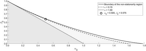
To further emphasize the different asymptotic behavior of when , consider here a small Monte Carlo study where i.i.d. realizations of are generated for large T. In particular, we consider the kernel density estimates for and against the normal density function which matches the (sample) median and interquartile range across Monte Carlo realizations. Specifically, we set , corresponding to approximately . This particular value is shown in Figure 1 , where we also show the values of corresponding to (), , as well as those satisfying (boundary of the non-stationarity region). The sample size T is calibrated such that the median number of durations in is about .

Details are in the caption following the image — **Figure 1**
Open in figure viewer PowerPoint

The stationarity region (gray) with lines indicating tail indices κ₀ = 1.00 and κ₀ = 0.15.

Figure 2 shows that, as predicted by Theorem 3 , the large sample distributions of both and display fatter tails than the Gaussian pdf.

Remark 5.It is important to note that for the case of , which is not ruled out by the ER conditions, the limiting behavior of is unknown (for both types of normalizations), even when is exponential (MLE). The key challenge in this case is that the large sample behavior of has not been established at present; see, for example, Mikosch and Resnick ( 2006 ). Also, we note that the results in Theorem 3 and its corollary hold only for the MLE. Further research is needed to understand the QMLE case.

4 Proofs and Additional Results

4.1 Proof of Lemma 1

We first consider the asymptotic behavior as for the score, the second-order derivative, and the third-order derivatives of . Next, we use these results to establish (i)–(iii).

Score: It holds that with

(11)

To see this, with c as defined in (C.4), let

, and decompose

where

and

. By conditions (C.1) and (C.4),

and

. Next, note that for any

Here,

by (C.4). Next,

by (C.1). As δ can be arbitrarily small, it follows that

Second-order derivative: Since (C.4) implies

, then by Gut ( 2009 , Theorem 2.1) it holds that (C.2) implies

(12)

Third-order derivatives: By (C.3),

(13)

and hence, since

, by (C.4) and again using Gut ( 2009 , Theorem 2.1),

Establishing (i)–(iii): These hold by using ( 11 )–( 13 ) together with the arguments in the proof of Lemma 1 in Jensen and Rahbek ( 2004 ), replacing T there by , and setting . Specifically, ( 11 ) replaces condition (A.1) in Jensen and Rahbek ( 2004 ), ( 12 ) replaces their condition (A.2), and ( 13 ) replaces their condition (A.3). Q.E.D.

4.2 Proof of Theorem 2

We verify conditions (C.1)–(C.4) in Lemma 1 for

, with

the log-likelihood in ( 3 ), and

in ( 1 )–( 2 ), with the corresponding counting process

. It is well-known that (i) and (ii) imply that

is strictly stationary and ergodic (and β-mixing with geometrically decaying rate); see, for example, Theorem 4.1.9 and Corollary 4.2.8 in Buraczewski, Damek, and Mikosch ( 2016 ) (henceforth, BDM) and Meitz and Saikkonen ( 2008 ). In particular, condition (C.1) holds by standard arguments (see, e.g., LH, proof of Lemma 9), and the strong LLN (see, e.g., Theorem 1 in Jensen and Rahbek ( 2007 )) applies, implying (C.2). For (C.3), let

, and

be strictly positive finite constants such that

, and

, and define the closed neighborhood,

Then, (C.3) follows as

with

strictly stationary and ergodic, by arguments as in Jensen and Rahbek ( 2004 , proof of Lemma 10).

In order to establish (C.4), note that since , we have , where the last term tends to zero a.s. (as , and hence, ). Hence, up to a negligible term, equals , which by Gut ( 2009 , Theorem 2.1) and the strong LLN converges a.s. to , as desired. Q.E.D.

4.3 Proof of Theorem 3

, then the information is random in the limit. The main challenge is to establish that, for the score and information,

(14)

where

is independent of the random variable

defined in Lemma 4 . Consistency and ( 9 ) then hold by an application of Kristensen and Rahbek ( 2010 , Lemma 12), together with the uniform convergence of the information.

To establish ( 14 ), we apply Theorem 3.1 in Sweeting ( 1992 ) which holds under the regularity conditions D1 and D2 therein. Specifically, condition D1 holds if (a.s.), under a sequence of data generating processes (DGPs) with true parameter value , . Let with . Condition D2 holds if, for any , , under the -sequences of DGPs.

To verify D1 in Sweeting ( 1992 ), note that by Lemma 4 ,

under

-sequences, and thus D1 follows by Slutsky's theorem provided

under

-sequences, as

. Let

denote a deterministic, positive, and integer-valued sequence for which

. As

, the desired result follows from Gut ( 2009 , Theorem 2.1) if

, under

-sequences as

. Here

, where

denotes the ith term of the second-order derivative of the likelihood function evaluated at

, and with the DGP generated by θ. We note

with

defined implicitly. Since

for T large, it follows that

, as

, by the uniform law of large numbers in, for example, Straumann ( 2005 , Theorem 2.2.1). Finally,

by dominated convergence as

when

To verify D2 in Sweeting ( 1992 ), note that by definition,

with

by Lemma 4 . Next, by the mean value theorem,

with

between θ and

. By arguments as in Jensen and Rahbek ( 2004 , Lemmas 7 and 9),

, with

stationary, ergodic, and all moments finite. Hence,

using Gut ( 2009 , Theorem 2.1) as

under

-sequences. Q.E.D.

4.4 Proof of Corollary 1

By the proof of Theorem 3 , , where Z is independent of . Moreover, , where ; this implies the desired result. Q.E.D.

4.5 Additional Lemma

Lemma 4.If and ,

(15)

where

is an almost surely positive

-stable random variable with parameter

the unique positive solution to

. The result in ( 15 ) also holds under

-sequences of DGPs.

Remark 6.We note that a κ-stable random variable is given via its characteristics function. It has right tail of the asymptotic order as ; see, for example, Samorodnitsky and Taqqu ( 1994 , Chapter 1) for more details.

Proof of Lemma 4 : By definition, at the true value

in ( 2 ) satisfies the stochastic recurrence equation

, with the i.i.d. sequence

. Since the function

, is convex with negative right derivative at 0,

, and

has infinite support, we have

, and there is a unique value

such that

. If

and

, an application of Hölder's inequality leads to a contradiction:

Hence,

, but

corresponds to the case

which is excluded as well. This proves that

. By Theorem 2.4.4 in BDM, with

it holds that

. Hence, by Lemma B.5.1 in BDM,

(16)

. Next, to establish ( 15 ) for

under

-sequences, introduce

. Define next

and, in addition,

. It follows that

Using the tail asymptotics ( 16 ) and mixing of

with geometric rate, by Theorem 9.2.1 in Mikosch and Wintenberger ( 2024 ),

, where

is a positive

-stable random variable. Hence, ( 15 ) holds with

, provided

for

. This again follows by noting that, by definition,

, such that for any

, by stationarity for T large enough,

With

. Next,

and

since

for T large as

. We conclude that

, which implies

by choosing ρ such that

. Q.E.D.

References

Buraczewski, Dariusz, Ewa Damek, and Thomas Mikosch (2016): Stochastic Models With Power-Law Tails. NY: Springer.
10.1007/978-3-319-29679-1
Google Scholar
Engle, Robert F., and Jeffrey R. Russell (1998): “Autoregressive Conditional Duration: A New Model for Irregularly Spaced Transaction Data,” Econometrica, 66 (5), 1127–1162.
10.2307/2999632
Web of Science® Google Scholar
Cavaliere, Giuseppe, Thomas Mikosch, Anders Rahbek, and Frederik Vilandt (2024): “Tail Behavior of ACD Models and Consequences for Likelihood-Based Estimation,” Journal of Econometrics, 238 (2), 105613.
10.1016/j.jeconom.2023.105613
Web of Science® Google Scholar
Gut, Allan (2009): Stopped Random Walks: Limit Theorems and Applications. NY: Springer.
10.1007/978-0-387-87835-5
Google Scholar
Jensen, Søren T., and Anders Rahbek (2004): “Asymptotic Inference for Nonstationary GARCH,” Econometric Theory, 20 (6), 1203–1226.
10.1017/S0266466604206065
Web of Science® Google Scholar
Jensen, Søren T., and Anders Rahbek (2007): “On the Law of Large Numbers for (Geometrically) Ergodic Markov Chains,” Econometric Theory, 23 (4), 761–766.
10.1017/S0266466607070326
Web of Science® Google Scholar
Kristensen, Dennis, and Anders Rahbek (2010): “Likelihood-Based Inference for Cointegration With Nonlinear Error-Correction,” Journal of Econometrics, 158 (1), 78–94.
10.1016/j.jeconom.2010.03.010
Web of Science® Google Scholar
Lee, Sang-Won, and Bruce E. Hansen (1994): “Asymptotic Theory for the Garch(1, 1) Quasi-Maximum Likelihood Estimator,” Econometric Theory, 10 (1), 29–52.
10.1017/S0266466600008215
Web of Science® Google Scholar
Meitz, Mika, and Pentti Saikkonen (2008): “Ergodicity, Mixing, and Existence of Moments of a Class of Markov Models With Applications to GARCH and ACD Models,” Econometric Theory, 24 (5), 1291–1320.
10.1017/S0266466608080511
Web of Science® Google Scholar
Mikosch, Thomas, and Sydney Resnick (2006): “Activity Rates With Very Heavy Tails,” Stochastic Processes and Their Applications, 116 (2), 131–155.
10.1016/j.spa.2005.08.003
Web of Science® Google Scholar
Mikosch, Thomas, and Olivier Wintenberger (2024): Extreme Value Theory for Time Series. Models With Power-Law Tails. NY: Springer.
10.1007/978-3-031-59156-3
Google Scholar
Samorodnitsky, Gennady, and Murad S. Taqqu (1994): Stable Non-Gaussian Random Processes. NY: Chapman and Hall.
Google Scholar
Straumann, Daniel (2005): Estimation in Conditionally Heteroscedastic Time Series Models. Berlin: Springer.
Google Scholar
Sweeting, Trevor J. (1992): “Asymptotic Ancillarity and Conditional Inference for Stochastic Processes,” The Annals of Statistics, 20 (1), 580–589.
10.1214/aos/1176348542
Web of Science® Google Scholar

The replication package for this paper is available at https://doi.org/10.5281/zenodo.13993686. The Journal checked the data and codes included in the package for their ability to reproduce the results in the paper and approved online appendices.

Volume93, Issue2

March 2025

Pages 719-729

A Comment on: “Autoregressive Conditional Duration: A New Model for Irregularly Spaced Transaction Data”

Abstract

1 Introduction

2 Main Result

3 Non-Standard Asymptotics

4 Proofs and Additional Results

4.1 Proof of Lemma 1

4.2 Proof of Theorem 2

4.3 Proof of Theorem 3

4.4 Proof of Corollary 1

4.5 Additional Lemma

References

Figures

References

Information

About Wiley Online Library

Help & Support

Opportunities

Connect with Wiley

A Comment on: “Autoregressive Conditional Duration: A New Model for Irregularly Spaced Transaction Data”

Abstract

1 Introduction

2 Main Result

3 Non-Standard Asymptotics

4 Proofs and Additional Results

4.1 Proof of Lemma 1

4.2 Proof of Theorem 2

4.3 Proof of Theorem 3

4.4 Proof of Corollary 1

4.5 Additional Lemma

References

Figures

References

Related

Information