Optimal Taxation of Income-Generating Choice
Abstract
Discrete location, occupation, skill, and hours choices of workers underpin their incomes. This paper analyzes the optimal taxation of discrete income-generating choice. It derives optimal tax equations and Pareto test inequalities for mixed logit choice environments that can accommodate discrete and unstructured choice sets, rich preference heterogeneity, and complex aggregate cross-substitution patterns between choices. These equations explicitly connect optimal taxes to societal redistributive goals and private substitution behavior, with the latter encoded as a substitution matrix that describes cross-sensitivities of choice distributions to tax-induced utility variation. In repeated mixed logit settings, the substitution matrix is exactly the Markov matrix of shock-induced agent transitions across choices. We describe implications of this equivalence for evaluation of prevailing tax designs and the structural estimation of optimal policy mixed logit models. We apply our results to two salient examples: spatial taxation and taxation of couples.
1 Introduction
Optimal income tax rates are shaped by the tradeoff between redistribution and economic distortion. The dominant framework for evaluating this tradeoff and deriving optimal income tax formulas assumes that agents are distributed across “smooth” hours or income choice problems indexed by an agent's preference or productivity type. However, many income-generating choices are naturally modeled as nonsmooth and discrete: where to live and work, whether to accept this job or that, whether to work full- or part-time. Integration of discrete income-generating choice into tax models permits analysis of the implications of adjustment along these margins for tax design. It further permits investigation of granular tax designs that reach beneath incomes to condition policy on underlying choices. But tax analysis in potentially unstructured discrete choice settings also presents challenges: optimal tax equations are complicated expressions leaving taxes implicit and often requiring evidence on cross-elasticities across many choice margins. We advance tax analysis in discrete choice settings by integrating the mixed logit, a flexible work horse demand/supply specification in applied microeconomics, into optimal tax theory. First, we use it to derive new expressions that describe the potentially rich aggregate substitution responses present in data. We show that these expressions encode behavioral responses to payoff variation as a Markovian “substitution” matrix. Second, we exploit the Markov structure of the substitution matrix to derive explicit expressions that connect optimal taxes to private substitution behavior and public redistributive goals. Third, we provide optimal tax equations for more structured discrete choice environments. We derive bounds for the coefficient from a regression of optimal taxes on incomes, which summarizes the overall redistributiveness of the tax code, and identify situations in which optimal taxes are monotone or convex in income. Fourth, we show in theory and in practice how the mixed logit formulation provides a clean identification of the substitution matrix and other structural parameters needed for policy analysis. Finally, we apply our results to two salient examples from the literature: spatial taxation and the taxation of couples.
In discrete choice supply models, a continuum of agents with heterogeneous preferences selects from a finite set of mutually exclusive income-generating activities. Choices may represent locations, occupations, skills, hours, pre-tax incomes, or combinations of the preceding. Each choice is associated with an after-tax income and an inherent amenity. Preference heterogeneity in combination with optimal choice behavior induces a distribution of agents over choices. Classic simple logit models generate preference heterogeneity via additive choice-specific preference shocks that are distributed according to a multivariate Gumbel distribution. Mixed logit models augment this with a further layer of preference shocks that enter utilities in a potentially general way. Prior work in discrete choice settings has identified the matrix of choice distribution derivatives (sensitivities) with respect to after-tax incomes as the essential behavioral component of optimal tax equations. This matrix describes the aggregate substitutability of choices and permits construction of the marginal excess burden of taxation. Formulas for simple logit choice distribution sensitivities are well known and formalize the strong restrictions on substitution behavior implied by this model. In contrast, while the mixed logit is known to permit rich substitution patterns, expressions for its choice distribution sensitivities have not previously been analyzed. We show that these sensitivities augment simple logit ones with an extra term that captures the extent to which different agent preference types regard pairs of choices as close substitutes and either cluster on or avoid both. Such behavior translates into elevated aggregate substitutability. We also show that the matrix of mixed logit choice distribution sensitivities has a surprising structure: It is the product of the transition matrix of an aperiodic, irreducible Markov chain and a matrix of marginal utilities of income. The former Markov matrix, which we call the substitution matrix and denote Q, describes choice distribution responses to tax-induced utility variation and is central to our analysis.
Discrete choice optimal tax equations resemble classic Ramsey commodity tax equations obtained in continuous choice settings. Like the latter, they express the marginal tradeoff between social redistributive goals and distortion that shapes policy design. However, also like the classic equations, they leave the structure of optimal taxes implicit. In addition, they require detailed information about behavioral adjustment along potentially many choice margins to evaluate existing or calculate optimal policy. In the latter case, this information is required at counterfactual equilibria. We confront these issues. First, we utilize the Markov structure of Q to invert the marginal excess burden component of mixed logit optimal tax equations. Compact expressions emerge that prescribe high taxes at choices attracting agents the policymaker seeks to extract resources from and that are close substitutes for other choices attracting such agents. Mean first passage times of Q are revealed to be the right way to formulate (lack of) substitutability and behavioral connectivity.1 Taxes are elevated when the covariance between mean first passage times and redistribution values is negative, where the latter summarize the the policymaker's desire to extract from those at a choice.
The optimal tax expressions described above place no assumptions on choices or preferences beyond the flexible mixed logit. Consequently, they are available for analysis in location, occupation, or other income-generating settings that lack natural payoff relevant structure. In some settings, however, tractability, a focus on salient choice margins, or prior quantitative work may motivate the adoption of additional restrictions. In exchange for a stronger separable mixed logit assumption and after breaking open redistributive values, we obtain an alternative optimal tax equation that formulates taxes as a fixed point of a contraction given Q. This permits a tighter connection between the pattern of optimal taxes and behavioral structure in Q. For the utilitarian simple logit case optimal taxes depending only upon incomes emerge. In particular, optimal income tax progressivity is entirely determined by the curvature of utility with respect to consumption no matter the structure of production or the pattern of amenity values. Thus, a researcher who adopts such a benchmark specification is a priori restricting themselves to an environment in which these features emerge. When utility is log-in-consumption, a common specification in applied work, but Q is unrestricted, the coefficient from a regression of (optimal) taxes on income is positive and bounds on its value in terms of properties of Q are available. This coefficient summarizes the overall redistributiveness of the tax code. Additional restrictions on Q supply cases in which optimal taxes are affine in income or are increasing in income relative to taxes paid at a salient “nodal” choice.2 In other separable mixed logit settings, we identify situations in which the structure of Q implies optimal taxes that are monotone in both choice and income or are progressive in income.
We next consider how to connect the possibly high dimensional Q to data, and hence, undertake quantitative evaluations of optimal taxes. In repeated separable mixed logit economies, this connection is very direct. The substitution matrix Q is the transition matrix describing the equilibrium evolution of agents across states in response to utility shocks. Intuitively, if shock-driven flows between two choices are large, then agents regard them as close substitutes, and consequently, a tax increment in one leads to a relatively large outflow to the other. Thus, if the data is generated by a repeated separable mixed logit, then an estimate of Q can be recovered from empirical flows of agents across choices. Such estimates can be used to construct empirical choice distribution sensitivities, and hence, evaluate the optimality of tax systems at prevailing equilibria.3 In addition, transition data supply moments for structural estimations of underlying preference heterogeneity parameters. The latter permit construction of maps from policy to choice distribution sensitivities, and hence, the calculation of optimal taxes at a given welfare criterion. The repeated mixed logit attributes persistent choice by a population of agents to the existence of (unobserved permanent) mixing types that favor particular choices and are rarely deflected by Gumbel shocks to alternatives. In such cases, substitutability in response to tax variation will be low. An alternative rationale for persistence is that Gumbel shocks describing modified circumstances or preferences are updated with low frequency and asynchronously. In this case, agents rarely move not because they are insensitive to payoff variation, but because their payoffs rarely change. Augmenting the mixed logit framework with such sticky payoffs does not modify the optimal tax theory previously developed, but does alter its connection to the data. We describe how transition data and short three period panels can be used to identify Q in this case.4
We put our results to work in illustrative spatial and couples hours choice applications. In our baseline spatial application, the choice set is identified with 100 urban and rural locations across the United States. We assume a sticky choice framework and disentangle the Poisson arrival rate of fresh Gumbel shocks and Q from short migration panels contained in the Survey of Income and Program Participation (SIPP) data. The derived Q matrix indicates complex substitution patterns across choices and provides prima facie evidence that the data is much better described by a mixed than a simple logit. Spatial choice is persistent, with most migration occurring between urban locations or within-state between urban and rural locations. Interstate rural-rural or urban-rural migrations are rare. We confirm that current U.S. taxes are consistent with a Pareto optimum for a large range of plausible marginal utility of consumption weights, but that rationalizing Pareto weights place relatively greater weight on the welfare of agents in high income urban locations. For a fixed utilitarian welfare criteria, we find support for a granular tax code that implements more spatial redistribution than occurs currently. Redistribution from high income urban locations is enhanced by substitutability with other other high income urban areas; redistribution to low income rural locations is tempered by substitutability with a local high income urban location. As an extension of our baseline application, we compute optimal spatial taxes for two different educational groups, no-college and some-college, subject to the raising of education-specific amounts of government funds. The latter are chosen to match the data with variation in them capturing (unmodeled) redistribution across education groups. The broad pattern of spatial taxes for each group resembles that in our baseline application, though with a shift in intercept when plotted against income. In addition, the taxes of the some-college group have a lower regression coefficient with respect to income and show more dispersion around the regression line than those of the no-college group. Our theory attributes this to less attachment and greater substitutability across locations among the college-educated.
In our application to the optimal taxation of couples, we suppose that each member of a couple can choose to work full-time, part-time, or not work creating nine possible hours choice combinations for couples. We identify Q with the transition matrix of couples across hours choices, recover this from Current Population Survey data and use it to inform structural estimates of couples' preference parameters. To a first approximation, we obtain optimal taxes that are monotone in household income, with modest but nontrivial deviations around an affine component. We interpret these results through the lens of our optimal tax theory for more structured settings: The Q matrix is close to monotone, translating into taxes that are close to monotone in household income. The regression coefficient of optimal taxes on household incomes is close to our upper theoretical bound indicating substitution behavior that compresses incomes toward their mean at a fairly uniform rate across choices. This behavior gives rise to the broadly affine shape. When we expand the model to allow for wage variation, we obtain an optimal tax code that depends not only on total household income but also on the distribution of incomes within the couple. In particular, given total household income, we find that it is optimal to give a tax deduction if the wife works.
Literature
A large literature considers optimal direct and indirect taxation in settings in which agents' choices respond smoothly to tax perturbations. In the context of income taxation, Mirrlees (1971) and Saez (2001) are seminal. Recent work by Lehmann, Renes, Spiritus, and Zoutman (2019) and Sachs, Tsyvinski, and Werquin (2020) extend the analysis of optimal direct taxation to rich income choice spaces and settings with endogenous wages, respectively. Seminal analyses of optimal commodity taxes include Diamond and Mirrlees (1971) and Diamond (1975). Atkinson and Stiglitz (1972, 1976) point out that while characterizing the distortions associated with optimal commodity taxation, these works offer limited characterization of the taxes themselves. They invert optimal commodity tax formulas to obtain further characterization in some cases. Saez (2002) recasts optimal income tax analysis in a discrete choice commodity tax framework and considers implications for EITC design. Saez (2004) shows that classical public finance results, such as production efficiency and uniform commodity taxation survive in a discrete income choice setting. Scheuer and Werning (2016) makes explicit the link between this framework and the continuum Mirrleesian model of optimal income taxation. Rothschild and Scheuer (2013) initiate a line of research in which agents make discrete occupational choices and continuous effort choices. See also Rothschild and Scheuer (2014), Ales and Sleet (2015), Gomes, Lozachmeur, and Pavan (2018), and Hosseini and Shourideh (2019). Each of these papers differs with respect to focus, the modeling of production, and the tax instruments available to the policymaker. However, in all of them agents have no inherent preferences over occupations: They select the occupation that maximizes their income and make small income adjustments in response to small tax changes. Laroque and Pavoni (2017) derive novel results on the optimal taxation of couples in a discrete choice model. Kroft, Kucko, Lehmann, and Schmieder (2020) introduce (one shot) search and imperfect labor market competition into a discrete choice tax model. Relative to these papers, our contribution is to derive optimal tax formulas and Pareto tax inequalities for mixed logit discrete choice settings that permit complex substitution and adjustment patterns across choices and incomes. Colas and Hutchinson (2021) and Fajgelbaum and Gaubert (2020) consider optimal tax design in spatial settings with rich production functions. Our quantitative spatial application relates to and complements this work by showing how to introduce potentially rich mixed logit preference structures into the analysis.
Layout
The remainder of the paper proceeds as follows. Section 2 introduces our baseline mixed logit environment and provides optimal tax conditions for this setting. Section 3 derives and interprets expressions for choice distribution sensitivities in simple and mixed logit settings. Section 4 embeds choice sensitivity formulas into the optimal tax equations from Section 2. Section 5 considers tax design in more structured settings. Section 6 describes how to connect Q to data. Section 7 deploys our approach to evaluate optimal policy design for the cases of spatial and couples taxation. Section 8 concludes.
2 Optimal Taxation in Mixed Logit Environments
This section lays out an equilibrium mixed logit environment and presents an optimal tax equation and Pareto test inequality for such a setting.
Individual Choice
 . Depending on context
  may represent a location, occupation, skill, hours choice, or income. Associated with each activity choice i is a pre-tax income
  , a tax
  , and an after-tax income
  . Thus, the granularity of taxes corresponds to that of the activity choice space and distinct choices associated with identical (or similar) pre-tax incomes may be taxed (very) differently.5 Agents derive utility from after-tax income and the innate amenity value of an activity choice. An agent's payoff from selecting i given after-tax income
  is
is

 denotes the agent's type and
  is assumed increasing and concave in its first (after-tax income) argument and to have continuous derivative
  in this argument. For a vector of after-tax incomes
  , we write
  as shorthand for the marginal utility
  at i. Given
  , a
, a  -agent solves
 (1)
(1) -type from a probability distribution μ. Such draws are independent across type components and across agents. The marginal distribution of μ with respect to β types has a density m, while the marginal distribution of each
  component is assumed to be a standard Gumbel.6 Together μ and the choice problems (1) define a mixed logit activity supply model. Given q, this model implies a distribution
  of agents over (payoff maximizing) activity choices, where for each i:
 (2)
(2) that are smooth in after-tax incomes and whose derivatives have a tractable form. These attributes have made the mixed logit a workhorse framework in modern applied microeconomics. Its use thus permits contact with a rich empirical literature that has supplied specification tests, estimation strategies, and identification arguments. Taken together these advantages make the mixed logit a natural framework for applied work in tax design.
 (3)
(3) in after-tax income. This case is consistent with a wide range of substitution responses to utility variation at a choice. But it implies that an after-tax income change at a choice induces identical utility variation for all agents selecting that choice. As described below, this facilitates nonparametric identification and sharpens theoretical results. Third, the mixed logit can be specified to approximate the Mirrleesian model with zero non-local cross elasticities. This is achieved by defining
  to be an ordered set of pre-tax incomes, imposing a single crossing property on u (with respect to i and β), and selecting u to ensure that variation in its values across choices is “large” relative to utility variation induced by Gumbel shocks.
Production and Equilibrium
A technology  converts allocations of agents across activities
  into final consumption good amounts. We assume throughout that F is increasing, has constant returns to scale, a continuous derivative
  , and satisfies an Inada condition. Given a vector of pre-tax incomes
  , a representative firm selects a demand allocation of agents
  to maximize profits
 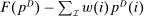 .
.
Let G denote exogenous government spending. A competitive equilibrium is a supply allocation of agents  , a demand allocation
  , a pre-tax income vector w, and a tax vector
  that is consistent with agent and firm optimality, market clearing, and policymaker budget balance. In particular, a competitive equilibrium
  satisfies:
  ,
,  ,
,  , and
, and 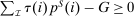 . Associated with any competitive equilibrium
  is an after-tax income vector
  . Combining the preceding conditions, using the constant returns to scale property of F, and substituting for q delivers an implementability condition that completely characterizes equilibrium after-tax income vectors.
Lemma 1.In the mixed logit environment with technology F, government spending G, and P defined as in (2),  is a competitive equilibrium after-tax income vector if and only if it satisfies the implementability condition:
 (4)
(4)Proof.See Online Appendix A.1. Q.E.D.
Optimal Policy
 satisfying (4)) is Pareto optimal if there is no implementable alternative
  such that
  with the inequality strict for some i. Let
 (5)
(5) may, after normalization by
  , be interpreted as the average marginal social welfare weight of those selecting i. In particular, for the case in which λ depends on β, but not ε, we have, via an envelope theorem, that:
  . Assume that a policymaker selects a competitive equilibrium to maximize the objective (5). Then, given Lemma 1, the policymaker's problem reduces to
 (6)
(6)Proposition 1.After-tax income vector  is Pareto optimal only if for all
  :
:
 (7)
(7) . An after-tax income vector q is a regular9 optimum at λ only if for all
  :
:
 (8)
(8) the average marginal social welfare weight of those selecting i, τ the optimal tax function, and ϒ the multiplier on
  at the optimum. In the separable mixed logit case,
 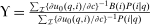 .
.
Proof.See Online Appendix A.1. Q.E.D.
Expression (7) provides a test of Pareto optimality that corresponds to being on the “right” side of the Laffer curve: if an equilibrium fails to satisfy (7), then it is possible to raise after-tax income at a choice, while simultaneously raising tax revenues. Expression (8) pairs a Pareto weighting density λ with an after-tax income vector q (and corresponding tax vector τ). It may be interpreted as a necessary condition for tax optimality at a given Pareto weighting or as a necessary condition for a Pareto weighting to rationalize the optimality of a given after-tax income vector.10 The left-hand side of (8) gives the net mechanical social benefit from slightly reducing  per member of the population at i. This benefit consists of the additional resources released for redistribution or government finance less the welfare loss to those agents choosing i. The reduction in
  induces choice adjustments. The right-hand side of (8) also gives the associated marginal deadweight loss.
Literature Connections
 (9)
(9) replaces
  and denotes aggregate demand for good i,
  is the aggregate compensated demand sensitivity for good i with respect to price
  , and
, and  augments marginal social welfare weights with terms that absorb tax revenue implications of individual level income effects. Note that in (9) Slutsky symmetry is used to replace
  with
with 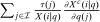 and formulate the aggregate behavioral response in terms of the impact on the demand for good i of adjustments in the price of all other goods j. The value of this classic formulation lies in its interpretation. The right-hand side of (9) is interpreted as the “discouragement” to the aggregate demand for good i stemming from a proportional adjustment in taxes. When agents are identical, the
  terms do not depend on i and this discouragement is equalized across goods. When agents are heterogeneous, the expression indicates that goods that carry smaller values of
  and that are consumed by agents with lower social marginal values of income are discouraged more. However, while expression (9) speaks to the optimal pattern of distortions, as various authors, for example, Atkinson and Stiglitz (1972), have noted, it is not especially informative about the structure of optimal taxes themselves. Atkinson and Stiglitz (1972, 1976) consider inversion of the matrix of compensated demand responses to obtain more explicit results for taxation. However, outside of special cases (e.g., two goods) this yields limited characterization.
In the discrete choice tax equation (8), the choice distribution sensitivities  correspond to uncompensated aggregate demand sensitivities. These are not generally symmetric:
  . However, a version of (9) is available by exploiting symmetry of choice probability sensitivities with respect to payoff variation. The next lemma specializes to the case of the separable mixed logit (3) and gives the result.11
Lemma 2.Assume a separable mixed logit. Let  and
and 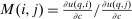 , then at a regular optimum:
 (10)
(10)Proof.See Online Appendix A.1. Q.E.D.
 into choice i consumption units) equals the social value of redistributing a dollar from those at i.12 However, while the formula (10) aligns with the well known optimal commodity tax formulas, the critique of Atkinson and Stiglitz (1972) that it carries limited information on the design of taxes themselves remains. In Section 3, we show that mixed logit choice distribution sensitivities
  have additional structure, which we use to unravel (8) and get sharper characterizations of optimal taxes.
Expressions (7), (8), and (10) indicate that in general all (own and cross) choice distribution sensitivities are needed to evaluate optimality of a given tax system. The applied researcher is often confronted with limited direct evidence on the response of agents to tax variation, which has occurred occasionally and along specific margins. Applied work has proceeded by a priori placing structure on choice distribution sensitivities. For example, in his analysis of income tax design, Saez (2002) focuses on the case in which activity choices are incomes and agents (can) only substitute between an income, neighboring incomes and nonwork so that for each  only
only  ,
,  are nonzero, that is, only “local” cross-elasticities and cross-elasticities with respect to inactivity are permitted to be nonzero. Restricting substitution patterns in this way is natural when the activity choice set is incomes and permits sharp results concerning Saez's targeted EITC application, but is less natural in the context of more complex and less structured activity choice sets. Recent contributions, particularly in spatial settings, have instead adopted the (conditional) simple logit preference model of MacFadden (1974). Colas and Hutchinson (2021) utilize this in their analysis of optimal income taxation in a discrete spatial setting, while Fajgelbaum and Gaubert (2020) augment it with endogenous amenity externalities in a model of optimal placed-based taxation. However, the simple logit structure (without mixing) also imposes strong a priori structure on choice distribution behavioral responses within conditioning populations, albeit a very different structure from that imposed by Saez (2002) or papers in the Mirrleesian tradition.
3 Mixed Logit Behavioral Responses
This section derives simple, interpretable expressions for behavioral responses in mixed logit settings. In particular, it shows that mixed logit models encode potentially rich empirical own and cross-substitution responses to granular payoff variation as a Markov substitution matrix. We heavily exploit this fact in subsequent optimal tax analysis.
Substitution in the Simple Logit
 . For
. For  ,
,  is the number of agents who, in response to an after-tax income increment at i, move from j to i expressed as a share of population at i. For
  , it is the number of agents who, in response to the increment, arrive in i from alternative choices again expressed relative to the population at i. The simple logit model delivers the following expression for these responses:
 (11)
(11) is the identity function that equals 1 if
  and zero otherwise. Expression (11) is simple, but also restrictive. In particular, it implies that a tax increment at i induces agents to depart i and move to alternative choices j in proportion to the population at these alternatives.13 To illustrate the strength of the restriction, consider the following scenarios.
Spatial Example.An economy's spatial choice set consists of two cities and many rural locations. Taxes are higher in the cities and lower elsewhere. Assume that in equilibrium the population divides with half locating in the two cities and the rest distributed uniformly across rural locations. A policymaker is considering whether to raise taxes in one of the cities. If the distribution of preferences is described by a simple logit, then a tax increment in a city will induce some of its residents to disperse to other locations in proportion to these other locations' populations. Two-thirds of the dispersers go to the low-tax rural locations and one-third to the other high-tax city. Given that the rural locations are taxed more lightly, this substitution will impose a relatively large loss in revenue (per dispersing agent). Suppose instead that the population is comprised of two groups. The first group prefers urban locations, concentrates upon the two cities, and regards them as close substitutes. The second prefers the countryside, concentrates upon the rural locations, and regards these as close substitutes. In this second scenario, a tax increment in one city will primarily push (first group) agents into the other high tax city. The loss in tax revenues associated with this substitution will be smaller. Assessing which substitution pattern prevails is important to the policymaker, but the second, while plausible, is a priori excluded by the simple logit specification.14
Substitution in the Mixed Logit
 with agents distributed over β types. Differentiating (2) and rearranging the expression for the derivative of P for this case delivers the behavioral response formula:15
 (12)
(12) and
and  ; the second group low. As a result,
  and
and  covary positively across β and the behavioral response
  is elevated. Economically, a utility increment at i draws a relatively large proportion of those types that find i attractive toward it. Since these types concentrate on j, it draws a relatively large fraction from j and the substitution response between j and i is large.16 The covariance term in (12) encapsulates these substitution patterns. In particular, the formulation is flexible enough to accommodate the alternative locational choice scenario described previously.
Formula (12) imposes structure on the matrix of behavioral responses: it has positive diagonal and negative off-diagonal elements. In addition, to this it implies that behavioral responses to utility variation can be encoded as elements of a Markov transition matrix Q. Moreover, the Markov chain corresponding to Q is aperiodic, irreducible, and reversible17 and has stationary distribution  equal to the choice distribution P.
Proposition 2.In the separable mixed logit model, the behavioral response of  with respect to a util increment at i is given by
 (13)
(13) (14)
(14) equal to P. The util behavioral responses in (13) are converted into after-tax income behavioral responses via multiplication by marginal utilities:
 (15)
(15)Proof.See Online Appendix A.2. Q.E.D.
 and
and  , where the matrix
  has rows equal to the choice distribution P. More generally, Q accommodates the richer substitution patterns permitted by the separable mixed logit model. As we discuss further below, the matrix Q has a second interpretation: In a repeated mixed logit setting, each row gives the choice distribution of agents following a fresh draw of Gumbel shocks conditional on current choice. We formally derive this and explore its implications for relating mixed logit tax models to data in Section 6.
In the general (nonseparable) mixed logit setting, marginal utilities of after-tax income vary by type. This adds a further layer to behavioral responses. Now an after-tax income increment at a choice i delivers different utility increments to different types. Substitution from one choice j to another i is elevated if types that concentrate on j also concentrate on i and those that concentrate on both have relatively large marginal utilities in choice i. Proposition 3 generalizes results from Proposition 2 to this case. As before, the matrix of behavioral responses has positive diagonal and negative off-diagonal elements and substitution patterns may be formulated in terms of the transition matrix Q of an ergodic chain. The matrix Q now incorporates the impact of marginal utility variation and need not have P as its stationary distribution.
Proposition 3.In the general mixed logit model, the sensitivities of P with respect to q are given by
 (16)
(16) and Q is an aperiodic, irreducible Markov matrix with unique stationary distribution
  not generally equal to P.
4 Optimal Tax Design for Unstructured Choice Environments
This section obtains an explicit characterization of optimal policy in mixed logit settings in which no restrictions are placed on  or the dependence of u on i. It is available for analysis of taxation in location, occupation, or other income-generating choice settings that lack natural payoff-relevant structure on choices.
Redistribution Vectors
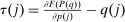
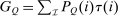
 (17)
(17) is the average marginal social welfare weight of those at i and
 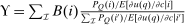 is the social value of a unit of resources distributed across choices so as to leave the choice distribution P unaltered.18 The term
  is the dollar value to society of redistributing an expected util's worth of resources from agents at i to the policymaker's budget. In the separable mixed logit model,
  reduces to
 (18)
(18) the average Pareto weight of such agents. Thus, θ describes the policymaker's desire to undertake marginal redistributions of welfare across populations concentrated on different choices at a prevailing allocation and exclusive of behavioral response considerations.
Optimal Tax Conditions in Terms of Q and θ
 (19)
(19) is the vector of reciprocal expected marginal utilities conditional on choice. In addition, substitution of Q and θ into the general optimal tax equation (8) implies
 (20)
(20) and Q, (19) permits testing of a prevailing tax system τ for Pareto optimality, while (20) permits computation of θ, and hence, via (17), recovery of the marginal social welfare weights that support τ as an optimum. Alternatively, (20) can be used to interpret an optimal tax system at a given welfare criterion by connecting it to a policymaker's desire to redistribute (the left-hand side is the redistribution vector) and agents' willingness to substitute across choices (the right-hand side is the normalized marginal excess burden of taxation). As in (8) and the classic continuous case (9), such interpretation is complicated by the implicit nature of (20).
Explicit Optimal Tax Equations
 to be the total revenues collected at
  , the (unique) stationary distribution associated with Q. Substituting this into (20) gives
 (21)
(21) is the stationary matrix of Q, that is, the matrix whose rows equal the stationary distribution
  , and e is the unit vector. Equation (21) has immediate implications for the simple logit case and highlights its salient role as a benchmark. In this case,
  and
and  , and hence, from (21),
 (22)
(22)More generally, it follows from (21) that variation in optimal taxes across choices is associated with variation in the elements of both θ and  . The ith element of
  gives the additional tax revenues generated when agents at i disperse across choices according to
  rather than the stationary distribution
  . Thus, (21) implies that taxes are higher at a choice i if tax-induced utility cuts lead agents to disperse to or remain in high tax choices (relative to the average implied by
  ). However, such destination choices are in turn high tax because they are associated with high redistribution values and high substitutability with other high tax choices. Unfolding this recursion and deriving a more explicit expression for optimal taxes can be achieved via “inversion” of the
  component of the marginal excess burden term in (20). Since Q is a Markov matrix and the matrix
  is singular, this inversion step requires a generalized matrix inverse concept called a group or Drazin inverse. Although an arbitrary square matrix X need not have a group inverse, matrices of the form
  , with Q the transition of an aperiodic, irreducible Markov chain, do. Further, their group inverses have the convenient form
 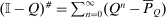 . We use this fact in Proposition 4 below.19
Proposition 4.Assume that agents are distributed across preferences according to a mixed logit model. At a regular optimum, taxes τ, redistribution vector θ, and corresponding substitution matrix Q satisfy
 (23)
(23) is the covariance between
  and θ under
  . In the separable mixed logit case, formula (23) holds with
  and
and  .
.
Proof.See Online Appendix A.3. Q.E.D.
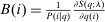
 -th element of
  gives the expected number of visits to j over N periods by an agent starting from i net of the expected number of visits unconditioned on any initial choice. As N becomes large this matrix converges to
  . The ith element of
 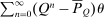 in (23) can then be interpreted as the expected social value of redistributing a util at each date from those who start at i to the general population if agents progress across choices according to Q.
The probabilistic interpretation of choice substitutability and its connection to taxation is sharpened by the next result, which relates optimal taxes to the mean first passage times of Q. Let  denote the
  -th mean first passage time of Q, that is, the expected number of periods before an agent at i “travels” to j under Q.21 In our context, mean first passage times may be interpreted as proxies for (cross) (in)elasticities: If
  is high, agents move infrequently between i and j (under Q) indicating limited substitutability between these choices. Proposition 5 provides a remarkably simple relationship between optimal taxes, mean first passage times of Q, and redistribution vectors. It asserts that taxes are higher at choices that have high redistribution values and that are behaviorally well connected to other high redistribution value choices. The latter connectivity is summarized by a smaller mean first passage time/redistribution value covariance, with low (resp., high) mean first passage times to high (resp., low) θ alternatives.
Proposition 5.Assume that agents are distributed across preferences according to a mixed logit model. At a regular optimum, taxes τ, redistribution vector θ, and corresponding substitution matrix Q satisfy
 (24)
(24) is the deviation-from-mean operator with
  and
and  is the (cross-)covariance vector with ith element the covariance between
  and θ under
  .
.
Proof.See Online Appendix A.3. Q.E.D.
Spatial Example (Revisited).The choice set  contains one city and one rural location. Pre-tax wages are exogenously given as 1 in the city and 0.8 in the rural location. Thus, all reported quantities can be interpreted as percentages of urban incomes. Agents have preferences net of Gumbel shocks of the form:
  . The policymaker attaches a Pareto weight of 0.94 to those who select cities and 1 to those who select rural areas. There is no government spending. Cases are distinguished by their β-type distributions.
Case 1. In the benchmark simple logit case, there is a single type  that values amenities in both locations equally. Results are given in Table I. In line with (22), optimal taxes equal redistributive values. In particular, the policymaker's concern for those who receive (Gumbel) preference shocks favoring the low wage rural location induces it to shrink moderately the 20% pre-tax city wage premium to a 14% post-tax consumption premium. The corresponding mean first passage times
  are independent of originating choices indicating that behavioral connectivity is uniform across these choices. The lower mean first passage times to the city reflects its greater attractiveness relative to the rural location.
Case 2. Assume that 50% of agents are urban types with  , while the remainder are rural types with
  . Urban types prefer the city, rural types the countryside on average. The values of β have been selected to generate exactly the same distribution of agents across choices
  as in Case 1 at the optimal tax levels from that case. Thus, given the Pareto weights from Case 1, a policymaker selecting taxes
  and viewing the resulting equilibrium through the lens of a simple logit model would conclude that they are at an optimum. However, this is not the case. Now, at the taxes selected in the first example, nearly 80% of city dwellers belong to the first β type and these agents are strongly attracted to high wage cities. Thus, if higher taxes are imposed in the city, relatively few agents will leave for the rural location. This permits the policymaker to undertake far more redistribution. Results for this case are reported in Table II.
The elevated mean first passage times between city and rural locations in this case relative to the last capture the reduced substitutability between these places underpinned by the types that concentrate upon them. Evaluation of the terms in (24) yields very similar values for θ terms and for the expectation 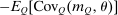 to those obtained in Case 1. However, the modified mean first passage times imply
  terms of 0.08 for the city and −0.06 for the rural region, reflecting the greater attachment of city and rural dwellers to, respectively, high and low redistribution value locations. Plugged into (24) these values yield taxes of 0.09 in the city and −0.11 in the rural area. Recognizing the strong attachment of most agents to urban or rural locations, the policymaker delivers consumption close to 0.9 for all agents and almost completely eliminates the urban consumption premium.
Case 3. This case shows how heterogeneity in substitution patterns can generate differential optimal taxation across identically earning choices. The choice set  now has four elements: two cities (labeled “PIT” and “PHL”) and two rural regions (labeled “near PIT” and “near PHL”) that are interpreted as local to one of the cities. As before incomes in cities equal 1 and in rural locations 0.8. Suppose four β types. The first two types are selected to have strong attachment to one city, weaker attachment to the other, and some attachment to the rural location near to the strong attachment city. The other two types have strong attachment to a rural area and some attachment to the local city. To introduce asymmetry across cities, types are selected so that local urban/rural attraction is stronger for PIT than for PHL. The results are reported in Table III. As before, the policymaker redistributes from those in cities to those in rural locations. But now the mean first passage times reflect the relatively greater attachment of those in PIT and near PIT to one another versus those in PHL and near PHL. This translates into a smaller covariance between mean first passage times and redistribution values, and hence, a smaller tax in PIT than PHL even though incomes and redistribution values are identical in the two places. Similarly, those in the rural vicinity of PIT receive a lower subsidy than those in the vicinity of PHL.
|
Case 1 |
||||||
|---|---|---|---|---|---|---|
|
τ |
θ |
|
|
|
||
|
City |
Rural |
|||||
|
City |
0.03 |
0.03 |
−0.01 |
3.74 |
4.30 |
0.53 |
|
Rural |
−0.03 |
−0.03 |
−0.01 |
3.74 |
4.30 |
0.47 |


|
Case 2 |
||||||
|---|---|---|---|---|---|---|
|
τ |
θ |
|
|
|
||
|
City |
Rural |
|||||
|
City |
0.09 |
0.03 |
0.08 |
3.75 |
7.92 |
0.53 |
|
Rural |
−0.11 |
−0.03 |
−0.06 |
9.05 |
4.29 |
0.47 |


|
Case 3 |
||||||||
|---|---|---|---|---|---|---|---|---|
|
τ |
θ |
|
|
|
||||
|
PIT |
PHL |
Nr PIT |
Nr PHL |
|||||
|
PIT |
0.063 |
0.057 |
0.007 |
4.18 |
5.55 |
4.08 |
6.22 |
0.239 |
|
PHL |
0.077 |
0.057 |
0.020 |
4.56 |
4.55 |
4.94 |
5.76 |
0.220 |
|
Nr PIT |
−0.052 |
−0.048 |
−0.003 |
4.16 |
6.02 |
3.52 |
6.46 |
0.284 |
|
Nr PHL |
−0.068 |
−0.048 |
−0.020 |
5.13 |
5.66 |
5.29 |
3.90 |
0.257 |


5 Optimal Tax Equations for Structured Environments
In this section, we place additional structure on payoffs and choices and derive further properties of taxes. In particular, we identify situations in which a regression of optimal taxes on incomes yields a positive coefficient and obtain bounds for that coefficient. We also identify situations in which optimal taxes are monotone or convex in income. Derivations in the previous section relied on the “inversion” of  in (20). In this section, we pursue an alternative path to elucidating the structure of optimal taxes that breaks open and inverts the redistribution vector θ component of tax equations. In exchange for a separable mixed logit assumption, this approach connects optimal tax variation across choices more tightly to income variation.
 , with
  increasing, strictly concave and twice differentiable, substituting the θ definition (18) into (20) and rearranging gives the optimal tax recursion:
 (25)
(25) defined implicitly and componentwise by
 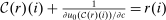 for
for  . The function
  is increasing with partial derivatives:
 (26)
(26)Simple Logit
We first use (25), the fact that  , and the policymaker's budget constraint to characterize optimal taxes in the benchmark simple logit.
Proposition 6.Assume a simple logit model with  and
and  increasing, concave, and twice differentiable. Given a utilitarian objective, optimal taxes are an increasing function of pre-tax income:
 (27)
(27) is convex and optimal income taxes are progressive if and only if
  is convex. Specifically, if
  and
and  , then optimal income taxes are progressive. If
  , then they are affine with marginal income tax rate
  .
.
Proof.See Online Appendix A.4. Q.E.D.
 and attitudes toward after-tax income. Thus, an applied modeler who selects such a specification is a priori restricting themselves to an environment that delivers these properties. This result holds independently of the production structure or of the direct dependence of
  , and hence, preferences, on i. It again relies on the fact that under simple logit the pattern of dispersal of agents across alternative choices following a decrease in after-tax income at a given choice i is independent of i.
Log-in-Consumption Utility
 unrestricted. We now reverse this and allow for general Q, but restrict
  to be log-in-consumption:
  . Such log restrictions are commonly made in applied work. In this case,
  and substitution into (25) gives
 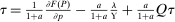 . Unfolding this recursion, assuming a utilitarian policymaker and substituting for ϒ yields
 (28)
(28) gives the vector of pre-tax income deviations from mean.22 Equation (28) relates optimal taxes to equilibrium income variation and substitution patterns and, in particular, implies that taxes are higher on choices that have high income deviations and are behaviorally well connected to other high income deviation choices at the optimum (with such connection now defined by Ω). It permits sharp characterizations of optimal taxes in some cases.
Locked and Floating Example.Consider an economy in which there are I “locked-in” types and one “floating” type. The ith locked-in type has a utility function that attaches arbitrarily large payoff to the corresponding choice i. This sticky type never leaves i and there is mass  of these types, with
  . The floating type has mass
  and distributes over choices according to P. The economy has substitution matrix
  . Since
  , it is immediate that
  . Thus, a util reduction at any i induces substitution behavior that shifts the income deviation from mean of agents at i from
  to a conditional expected income deviation from mean of
  . Conditional expected income deviations from mean are, thus, uniformly compressed toward zero by payoff reductions and this uniform compression underpins linear taxation in Δw. Substitution for Q in (28) yields:
  , and hence, a marginal income tax of
  . This marginal income tax is increasing in ψ reflecting greater redistribution when choice is more persistent and less elastic.
Nodal Choice Example.In the leading example of Saez (2002), unemployment acts a nodal state: agents can substitute between unemployment (the node) and positive earning occupations, but not between different occupations. Analogously, suppose there is a “nodal” choice  such that
  unless i or j equal 0.23 In this case, (28) reduces to, for
  ,
,
 (29)
(29) and for
  ,
, 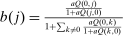 . Thus, taxes relative to those at the nodal choice increase with earnings. Nonlinearities in this relationship are introduced by variations in
  and the extent to which choices are behaviorally connected with the nodal choice. Optimal taxes at i are below those at the nodal choice if earnings at i,
  , are below mean earnings
  , where the latter mean is computed using behavioral connectivity weights b. In particular, if the nodal choice is behaviorally well connected with higher earnings choices, then this mean will be larger and taxes at low earning choices will be below those at the nodal choice. This type of result emerges in Saez (2002), where (the nodal choice) unemployment is better connected to higher earning choices than are low earning occupation choices and taxes on the former are correspondingly higher.
The locked and floating example above is a particular case in which Δw is an eigenvector of Q (with eigenvalue ψ). Whenever this situation arises, the substitution behavior encoded in Q will imply uniform compression of income deviations Δw to zero and (with log-in-consumption utility) an optimal marginal income tax rate  . We formalize this result in Online Appendix A,24 where we give other economic examples in which Δw is an eigenvector of Q and optimal affine income taxes emerge. This situation is, however, more likely the exception than the rule. In general, variation in substitution behavior at different choices implies nonuniform variation in the speed with which income deviations converge to zero, and hence, departures from affine income taxes. However, even in these cases the eigenstructure of the substitution matrix Q can be used to bound the coefficient from a regression of (optimal) taxes on income. This coefficient gives the slope of the “affine component” of optimal taxes (with respect to income) and is a useful measure of the overall redistributiveness of the tax code. Proposition 7 shows that this coefficient is always positive and has a lower bound closer to one the more persistent is choice and the closer the diagonal elements of Q are to one.
Proposition 7.Let ρ be the coefficient on pre-tax income from a population regression of optimal taxes onto a constant and pre-tax income. Then  , where
  and
and  are, respectively, the smallest and second largest eigenvalue of Q.
Proof.See Online Appendix A.4. Q.E.D.
Separable Mixed Logit
We now depart from the log-in-consumption case and return to (25). This departure introduces nonlinearity into reciprocals of marginal utilities (i.e., the prices of goods in terms of utils), and hence, into the relationship between redistribution vector elements and after-tax incomes. This in turn introduces additional nonlinearity into the relationship between optimal taxes and incomes. However, in the presence of income effects and strict concavity of  , the recursion defined by (25) inherits a contraction-like property from the dependence of marginal utilities, and hence, redistribution values on after-tax incomes. This permits characterization of tax designs in separable mixed logit settings without log utility.
Lemma 3.Assume a separable mixed logit model with  and
and  increasing, strictly concave, twice differentiable and with the slope of:
  bounded below by
  . Let τ be an optimal tax function at Pareto weights λ, with corresponding equilibrium pre-tax incomes
  , substitution matrix Q, and multiplier ϒ. Define the operator
  by
by
 (30)
(30) . Then
  is a contraction on
  with modulus
  and τ is the unique solution to
  .
.
Proof.See Online Appendix A.4. Q.E.D.
Remark 1.The lemma addresses two technical details. First,  is defined only on
  . To ensure that the map
  is defined on all of
  (including at tax vectors τ implying negative consumptions at some choices), the extension
  of
of  onto all of
  is used in (30). Second, to ensure that the slope of each
  , and hence,
  has modulus less than one, we require that the slope of
  is uniformly bounded from zero. This assumption is satisfied by many utility functions or by slight perturbations of them. The assumption implies that redistribution values are strictly increasing.
In the remainder of this section, we leverage Lemma 3 to relate properties of Q to those of τ at an optimum. We then describe conditions on utilities that deliver relevant properties of Q globally (i.e., at all tax policies), and hence, at the optimum. We begin by placing an order on the choice set  and seeking conditions that ensure monotonicity of taxes in this ordering. For concreteness, suppose that
  is a collection of points in
  with each component of
  indexing the quantity of a particular choice attribute. For example, i could be a vector of hours worked by family members with
  the amount worked by household member m or i could be a pair of elements indicating an occupation and a (discrete) hours choice. Assume that
  inherits the usual partial order from
  25 and define a set
  to be increasing if
  ,
,  and
and  , implies
  . The matrix Q is increasing if
  implies for each increasing
  ,
,  . In other words, Q is increasing if agents selecting high-valued choices are more likely to regard other high-valued choices as close substitutes than those selecting low-valued choices.26 If
  , Q is increasing if
  implies that
  first order stochastically dominates
  .
.
Proposition 8. (Monotonicity)Let the conditions of Lemma 3 hold. Let τ be an optimal tax function with corresponding equilibrium pre-tax incomes  and substitution matrix Q. If the choice set is partially ordered, w is increasing, and λ nonincreasing in choice, and Q is increasing, then the optimum is attained by a tax function increasing in choice. If
  , then the optimum is attained by an increasing income tax function.
Proof.See Online Appendix A.4. Q.E.D.
 .
.
Lemma 4.Assume that  is totally ordered,
  and that
  is supermodular in
  , then in any equilibrium and, in particular, at the optimum Q is increasing. Further, in combination with the assumptions of Proposition 8, the optimum is attained by an increasing income tax function.
Proof.See Online Appendix A.4. Q.E.D.
The assumption of Lemma 4 is standard in Mirrleesian optimal income tax and many contracting problems. In particular, if  is twice differentiable on
  , supermodularity amounts to assuming that
  , which is satisfied by, for example,
  . In Online Appendix A.5, we describe a “fuzzy Mirrlees model” in which an underlying Mirrleesian preference structure satisfying the conditions of Lemma 4 is augmented with Gumbel shocks. The latter imply that while higher β types tend to cluster on higher (income) choices, there is dispersion of them across other choices and not all substitution behavior is local. Nonetheless, consistent with Lemma 4 optimal taxes are monotone.27
We next consider assumptions that refine those in Proposition 8 and imply optimal progressive income taxation. The additional condition is a convexity requirement on Q. Suppose that  is totally ordered and define the conditional survival functions implied by Q according to
  . We say that Q is convex if for each
  and
and  ,
,  is increasing in i. This is the discrete analogue of the requirement that the survival functions associated with Q are convex in their conditioning argument. It implies that increases in i not only raise the probability of substitution into higher ordered choices (as under increasingness), but do so at an increasing rate.
Proposition 9. (Convexity)Let the conditions of Proposition 8 hold. Let τ be an optimal tax function of a utilitarian policymaker with corresponding equilibrium pre-tax incomes  and substitution matrix Q. If
  and is totally ordered, w is linearly increasing in i,
  is convex, and Q is increasing and convex, then the optimum is attained by an income tax function that is increasing and convex in income.
Proof.See Online Appendix A.4. Q.E.D.
 that imply convexity of Q and, hence, with the other conditions of Proposition 9, convexity of taxes in income.
Lemma 5.If, in addition to the conditions on  in Lemma 4,
  and
and  is increasing in β, then Q is convex. In combination with the other assumptions of Proposition 8, then the optimum is attained by a convex and increasing income tax function.
Proof.See Online Appendix A.4. Q.E.D.
 is met in many applications in which i is income or effort. The additional requirement
  ensures that higher β types cluster on higher ranked choices at a faster rate. It holds if, for example,
  , with
  and
and  . In Online Appendix A, we give an example of a “fuzzy Mirrlees” model with convex optimal taxes.
6 Connecting Mixed Logit Behavioral Responses to Data
Quantitative evaluation of the optimality of tax systems using expressions (23) or (25) requires estimates of the corresponding substitution matrix Q and vector of conditional marginal utility reciprocals  . This is complicated by the fact that Q is a potentially high-dimensional object describing adjustment to utility variation along many margins. In this section, we provide results on the identification and estimation of Q, marginal utility parameters, and other deep structural parameters. Each of these results exploits the model-implied connection between preference shock induced choice transitions and substitution in response to tax or income variation.28 First, we show that, under the assumption of a repeated separable mixed logit model, Q is nonparametrically identified and recoverable from equilibrium transition data. Combined with marginal utilities, estimates of Q permit construction of the entire matrix of choice distribution sensitivities at an equilibrium, and hence, evaluation of an existing tax system. If utilities are given by
  , then marginal utilities (of after-tax income) are parameterized by a and estimates of the matrix of choice distribution sensitivities may be built from those of a and Q. We show in the Appendix in the Online Supplementary Material that estimates of a may be recovered from data on the impact of after-tax income variation on choice shares at a potentially limited number of choices. Full structural approaches to modeling and estimating agent choice place low-dimensional parametric restrictions on u and m. Estimates of these parameters may be used to construct the entire choice distribution map
  and its sensitivities, and hence, evaluate these sensitivities at counterfactual allocations and undertake optimal tax analysis at fixed Pareto weights using (23) or (25). Our second result describes how transition data provides an extra set of moments that can be used to discipline such parametric estimates.
We then describe an extension of our baseline framework that permits better contact between the framework and data while preserving the underlying tax theory. This extension supposes Gumbel preference shocks that persist and that are updated randomly and asynchronously across agents. Our baseline repeated mixed logit attributes persistent choice by a population of agents to the existence of (unobserved permanent) mixing types that favor particular choices and are rarely deflected by Gumbel shocks to alternatives. In such cases, substitutability in response to small tax-induced payoff variation is low. An alternative rationale for persistence is that Gumbel shocks describing modified circumstances or preferences are updated with low frequency and asynchronously. In this case, agents rarely move not because their behavior is insensitive to payoff variation, but because their payoffs rarely change. Incorporating such sticky payoffs and correspondingly sticky choices into the mixed logit structure does not modify the optimal tax theory previously developed, but does alter its connection to the data. Our extension describes how transition data and short three period panels can be used to identify Q in this case.29
6.1 Identification of Separable Mixed Logit Parameters
Nonparametric Identification of Q at an Equilibrium
Consider a repeated version of the one shot separable mixed logit choice environment considered previously. Agents face a time invariant after-tax income function q, draw a permanent β type at the beginning of their lives, and a fresh ε type in each period. They face no costs of choice adjustment. An agent's current payoff is then independent of past choices and its problem reduces to a repeated static one of the form (1). In this repeated economy, agents migrate across choices when they draw new Gumbel shock vectors that alter their optimal choice. Because different choices i tend to attract different β-agent populations (who visit alternative choices with different probabilities), this repeated model gives rise to a Markov matrix describing observed transitions between choices. This Markov matrix is exactly the substitution matrix Q defined in (14). It follows that in this case Q is identified by observable choice transitions. The proof of Proposition 10 formalizes the argument.
Proposition 10.Let  denote the transition matrix of agents across choices, with
  the fraction of agents that move from i to j in a period. In a repeated separable mixed logit choice environment,
  equals the substitution matrix Q.
Proof.See Online Appendix A.6. Q.E.D.
The separable mixed logit model places some structure on the substitution, and hence, the transition matrix. In particular (see Proposition 2), it implies that Q is the transition of a reversible Markov chain, and hence, is such that for all i and j,  . Trendelkamp-Schroer, Wu, Paul, and Noe (2015) describe maximum likelihood estimators for reversible Markov chains that are applicable to raw transition data. These may be used to recover an estimate of Q that satisfies reversibility.30 To build the matrix of choice distribution sensitivities, estimates of marginal utilities (of after-tax income) are also required. If utilities are given by
  , then these marginal utilities are parameterized by a. We show in the Appendix that estimates of a may be recovered from data on the impact of after-tax income variation on choice shares at a potentially limited number of choices.
Disciplining Structural Estimates With Transition Data
 is posited, where
  is a vector of observable choice attributes associated with the jth choice, β is a corresponding vector of preference types with ⊤ a transpose, and
  is an unobserved amenity value common to those selecting j. Included in x is a function of pre-tax income, for example,
  . Agent types have the form
  , with ν distributed according to a mean zero density
  with parameter ϕ. A separable mixed logit model is obtained by assuming the density over the β component associated with q is degenerate. Let
  denote a reference choice,
  the set of remaining choices, and
  the mean utility available at choice j relative to the reference choice, with
  and
and  . The choice distribution P is related to Δu and the density parameter ϕ via

 denote the inverse of
  at the empirical choice distribution
  . The standard approach proceeds by recovering
  and then solving
 (31)
(31) satisfying
  . The standard approach does not utilize transition data. However, the repeated mixed logit model implies, in addition, that flows between choices satisfy
 (32)
(32) also equaling the substitution matrix in the separable mixed logit case. Equation (32) supplies an additional set of moment conditions that may be used to supplement the moment conditions (31) and further discipline the parameter estimates
  . In Online Appendix C, we describe how to integrate these additional moments into the estimation procedure in the context of particular applications. These moments assist in identifying structural parameters by revealing choices, and hence, observable choice attributes whose valuations are highly correlated across agents in the data.31
6.2 Sticky Choice
We now describe a sticky choice extension of our baseline framework.
Sticky Shocks and Sticky Choice
 in a period. As before, β types are permanent. Assuming a separable mixed logit structure and a utility discount factor of ρ, agent lifetime payoffs evolve according to

 . The agent's choice problem remains a static one with each agent repeatedly selecting the same activity until they draw a new preference shock. The (stationary) choice distribution is given by (2), choice sensitivities by (15), and the substitution matrix by (14). Expressions for the marginal excess burden and optimal tax equations evaluated at stationary choice distributions are unchanged. Now, however, the transition matrix of agents across choices no longer equals the substitution matrix Q. Instead it is given by
 (33)
(33)Lemma 6.For a triple of choices  , let
, let  denote the probability that an agent in i transitions to j and then to k given q. We have that for each pair of choices
  :
:
 (34)
(34)Proof.See Online Appendix A.6. Q.E.D.
 and
and  involve agents starting in i and spending subsequent periods in i and j. However, they differ in the timing of the visit to j:
  involves remaining in i and then visiting j, while
  visiting j and then returning to i. Since the
  path involves two transitions, it must also involve a drawing of Gumbel shocks in each successive period. In contrast, the
  path may have involved two draws with the first leaving i still optimal, but it may also have occurred via no redraw followed by a draw that renders j optimal. This second possibility elevates the probability of the
  path and permits identification of
  . Once d has been estimated from panel data via construction of the empirical counterparts to the moments in (34), the substitution matrix may be disentangled from
  using (33).
7 Quantitative Applications
This section provides two illustrative applications of the mixed logit framework to tax design problems. The applications highlight the framework's flexibility and potential to consider granular tax designs that reach beneath income and attach taxes to income-generating choice. Our first application analyzes the structure of optimal place-based tax policy in the United States. Our second considers the optimal taxation of couples.
7.1 Optimal Place-Based Taxation
We model agents as selecting a location to live and work given their assessment of location specific after-tax incomes and amenities. The U.S. Census provides information by county on the fraction of people living in an urban environment. We classify a county as urban if 70% of its inhabitants are classified as urban and as rural otherwise. We combine urban counties within a state into one location and rural counties into another. All counties in Maine are classified as rural, while the District of Columbia is classified as a fully urban area. We identify the choice set  with the resulting collection of 100 U.S. urban and rural locations. The policymaker selects location-specific taxes. This application is a natural candidate for our flexible mixed logit approach since it involves a large unstructured discrete choice set with no clear a priori reason to favor one preference distribution over another. Recent work on optimal taxation in spatial settings has been done by Fajgelbaum and Gaubert (2020) and Colas and Hutchinson (2021), who build on the location choice model of Diamond (2016). Relative to these papers we simplify the production side of the economy, but enrich the preference side by considering a rich mixed logit structure.
Recovering the Substitution Matrix
Our initial step is recovery of the substitution matrix Q from transition data. We first utilize the procedure of Trendelkamp-Schroer et al. (2015) and fit a reversible Markov chain  to IRS location-to-location migration data counts for the years 2017 and 2018.33 Both the raw count data and the fitted reversible chain exhibit significant persistence. To disentangle persistence due to preference attachment from that due to inertia and stickiness in circumstances, we assume the data is generated by the sticky choice model described in Section 6. Then
  and Q are related by
  . To estimate the Poisson arrival rate d of fresh Gumbel shocks, and hence, recover Q from
  , we implement the procedure described in Section 6.2. For this, we use the short migration panel contained in Survey of Income and Program Participation (SIPP) data for the years 2013 to 2016. Further details of the estimation procedure are reported in Online Appendix C. We obtain
  . This value is combined with the estimate of
  and the expression
  to generate an estimate of Q.
Analysis of the Substitution Matrix
The estimated Q matrix indicates rich substitution patterns across locations. Figure 1 illustrates some of these by organizing locations into rural and urban blocs and then within each bloc alphabetically ordering locations by state. Elements of the estimated Q matrix in excess of 0.01 are displayed. Thus, for example, displayed elements in row 5 show locations that those in rural California transition to with probability in excess of 0.01; elements in row 55 do the same for urban California. The figure indicates that larger elements are found on the main diagonal (staying in place), an upper diagonal (substituting within-state from a rural to an urban location), and a lower diagonal (substituting within-state from an urban to a rural location). The lower right-hand quadrant is more densely populated with transitions in excess of 0.01 indicating a higher rate of substitution between urban locations. Interstate rural-to-rural, rural-to-urban, or urban-to-rural substitution is rarer. The overall pattern of substitution is inconsistent with a simple logit preference structure, which would imply identical Q rows and substitution patterns independent of originating location.

Elements of Q greater than 0.01.
Detailed inspection of substitution patterns into and out of particular states reveals further complexity. Figure 2 displays the estimated Q's mean first passage times from urban areas of states to urban California. The figure indicates that substitutability has a gravity-like aspect: urban areas further from California tend to have higher mean first passage times to urban California. This pattern is replicated for other locations: a regression of log of mean first passage time on log of location-to-location distance (together with a set of dummy variables for the destination) yields a coefficient on the log-distance equal to 0.329 (0.01).34 However, the relationship between mean first passage times and distance is imperfect. For example, distant, but relatively high income urban areas in states like Massachusetts have lower mean first passage times to California than closer, but lower income urban areas in states like Mississippi or Louisiana. Overall, the Q matrix and its implied mean first passage times point to complex substitution patterns that can be accommodated by a mixed logit, but are less obviously captured by simpler preference structures.

Log mean first passage time to urban California from other urban locations.
Evaluation of the Current Tax Code
 , the Pareto inequality (19) holds if

 . Our subsequent benchmark estimate of a is 4.29. We conclude that variation in average household taxes across states is consistent with Pareto optimality. We next turn to (20) and use the estimate of Q to recover redistribution vectors θ that rationalize observed taxes as optimal. From these, we construct rationalizing Pareto weights by inverting the definition of θ:
  , where again
  is assumed. Figure 3 plots the resulting Pareto weights against values for average household pre-tax income (with California's weight normalized to one). The figure reveals a positive correlation between state-level Pareto weights and average household incomes (with DC an interesting outlier). This correlation implies that, relative to a utilitarian criterion, the U.S. political process overweights high income states.35 Intuitively, relatively small transition probabilities mainly to other similarly taxed locations imply moderate tax revenue sensitivities. These are small enough for a utilitarian policymaker to seek further spatial redistribution than is supplied by current U.S. taxes. The model reconciles U.S. taxes with empirical substitution patterns by deducing state level Pareto weights that correlate positively with average state household income and that remove such redistribution motives.
Relationship between implied Pareto weights and income.
Structural Mixed Logit and Optimal Taxes
 (35)
(35) is a common-across-agents preference fixed effect for choice i,
  is the value of choice characteristic s at i and
  is the idiosyncratic marginal value of these choice characteristics to an agent. Choice characteristics
  are identified with dummies indicating locations, groups of locations, and rural-urban characteristics. The distribution of β is parametrized by a vector ϕ. Assuming a utilitarian policymaker and after substitution for
  , (25) implies
 (36)
(36) . We assume that the production function is linear in inputs, treat incomes
  as exogenous and identify them with average pre-tax incomes by location in 2018.36 We obtain estimates of a and ϕ via the procedure described in Section 6.1. Our estimated value for a in this case is
  . Further details of the data, specification, estimation procedure, and calculation of optimal taxes are given in Online Appendix C.
Results
Figure 4 displays the optimal mixed logit tax code as a scatter plot against income at the location level (dot). For comparison, the current U.S. tax code is plotted (triangle). The optimal code under the utilitarian objective implies significantly more redistribution across locations than occurs under the actual U.S. tax code. This result mirrors our earlier observation that to reconcile the optimality of the existing code with a mixed logit specification requires replacement of utilitarian societal preferences with less redistributive ones. Table IV summarizes implications of the optimal tax function for rural/urban redistribution. It implies an increase in the average urban tax liability of $2503 and a reduction in the average rural tax liability of $7990 relative to empirical values (in 2018 dollars). The average after-tax urban income premium is reduced from 26% to 13%.

Tax schedule: optimal versus data. Values in 2018 dollars.
|
Data |
Optimum |
|
|---|---|---|
|
Average Urban Tax Liability |
$13,509 |
$16,012 |
|
Average Rural Tax Liability |
$6617 |
|
|
After Tax Urban Premium |
1.26 |
1.13 |
|
Rural Pop (%) |
22.1 |
23.2 |


 and is a force for higher taxes and lower after-tax incomes in NH (dampened and slightly offset by the difference in redistribution values:
  ).
).
Deviation from affine tax code for U.S. states.
 :
:

7.2 Optimal Place-Based Taxation by Educational Group
The preceding analysis abstracts from within-location income heterogeneity. In this section, we compute optimal spatial taxes for different educational groups whose different earnings contribute to such heterogeneity.
Following Diamond (2016), we subdivide the population into two educational groups, categorizing individuals as low educational attainment if they have a high school degree or less and high educational attainment if they have at least some college education. We utilize cross-state migration rates by education provided by the U.S. Census for the years 2007 to 2011 to construct Q. This requires us to redefine choices as states rather than urban or rural locations within states. We complement this data with income and imputed taxes from the March CPS of the same years.37 Interstate migration patterns differ by educational attainment. In particular, more educated individuals are more mobile: 89% of high educational attainment agents remain in place from one year to the next compared with 93% of low educational attainment agents. Given this, and proceeding as before, we estimate a separate set of locational preferences for each educational group. We set per capita, education-specific government tax liabilities equal to their corresponding values in the data:  for the low education group and
  for the high education group. Thus, the tax reform we recover is optimal across locations for each educational group conditional on these education-specific funding requirements.38

 indicating less variation in income across the sets of states considered close substitutes to VT and AL, respectively.
Deviation of optimal taxes from affine code conditioning on education levels.
7.3 Optimal Taxation of Couples' Labor Supply
The labor supply of a couple each of whose members can work no time (L), part-time (M), or full-time work (H) provides a second natural example of a discrete income-generating choice.39 Following Hoynes (1996), we identify  with the resulting set of 9 possible couples' hour combinations. Under the assumption of a repeated separable mixed logit, a reversible Markov chain fitted to the transition matrix of agents across hours choices provides an empirical proxy for the substitution matrix Q. We use the CPS from 2010 to 2019 to generate the transition matrix and fit a reversible Markov chain. Figure 7 displays the results. The figure indicates variation in the rows of Q and, in particular, persistence of choices. As for the spatial case, this pattern is inconsistent with a repeated simple logit model, which would imply distributions of hourly choices independent of the previous choice. It provides prima facie evidence for a repeated mixed logit in which some mixing types are strongly attracted to particular hours combinations. The estimated Q reveals further interesting and tax design relevant labor supply substitution patterns. For example, choice persistence is weakest for hours combinations involving part-time work (M). This implies greater willingness of part-time workers to substitute into other hours options following a part-time payoff reduction and, corresponding, less willingness of full- or no time workers to substitute following a payoff reduction.

Q implied by CPS transition data. Labels H, M, L denote full-, part- and no time labor supply for the husband and wife, respectively. Rows ordered by total household income.
As in the spatial application, optimal tax analysis requires a structural estimation of preference parameters. We adopt the preference specification (35) and identify the choice characteristics  with dummy variables indicating whether a choice involves full-, part-, or no time work by each spouse. The distribution of β preference types is assumed to be a multivariate normal
  . We evaluate optimal taxes via (36) with G set equal to
  (in 2010 dollars) and w to the average wage and salary income earned by couples at each hours combination. The parameter a is estimated to be
  . Further details of the data, estimation procedure, and calculation of optimal taxes are given in Online Appendix C.
Results
 and increasing set
  that
that  . We find that this inequality holds for 651 out of 684
  combinations in our example. Thus, in most cases couples who choose higher income hours combinations are also more likely to substitute into other higher income combinations. This pattern, in combination with marginal social welfare weights that decline with income, underpins the near monotonicity of optimal taxes in income. Proposition 7 supplies bounds for the population regression coefficient of taxes on incomes. In the current example, these bounds are

 and
and  are the smallest and second largest eigenvalues of the optimal Q matrix. The coefficient ρ is very close to the upper bound. Relatedly, the vector Δw of deviation-from-mean incomes is close to the eigenvector associated with
  . In economic terms, couples who substitute from choices tend to compress income deviations from mean at a fairly uniform rate across the choice space. In conjunction with the log utility assumption, this imparts the affine component to optimal taxes.
Optimal taxes.

 at (M/M). Substitutability between
  and high θ states is greater than for
  and this promotes taxation at
  .
.Income Variation Within and Across Hours Choices
The preceding results abstract from income variation among agents making the same hours choice. This obscures the differential tax treatment of couples who earn the same household income through different household labor supply combinations. If two couples file the same income, should the distribution of hours (and incomes) across the couples' members qualify one for a tax deduction? To evaluate this, we implement an extension of our baseline model in which couples randomly draw a wage for each member and then select among hours. Equivalently, they select from the random discrete income sets implied by their wage draw and hours options. This framework can be accommodated in our mixed logit framework by treating spousal income pairs as a choice and wages as an additional mixing variable. Details are given in Online Appendix C.
 (37)
(37)
Optimal couple taxation.
8 Conclusion
The mixed logit has emerged as a workhorse demand/supply specification for modern structural equilibrium discrete choice models. It accommodates environments in which agents solve non-smooth discrete choice problems on potentially unstructured choice sets and in such settings allows a flexible modeling of substitution responses to after-tax price changes. These elements permit a rich modeling of income-generating choice and its response to tax variation. This paper connects the tools of applied discrete choice analysis to optimal tax theory. It provides new tax formulas oriented toward helping practitioners interpret their results and understand the role of a priori assumptions in shaping those results. In a mixed logit setting, the key behavioral responses required by optimal tax formulas are related to a Markov substitution matrix. This connection permits derivation of “inverted” optimal tax equations that relate optimal taxes to the interaction of public marginal redistributive objectives and private substitution behavior, with the latter summarized by mean first passage times between choices. In more structured settings, conditions for optimal taxes to be monotone in choice or income, affine or convex in income are identified. In some settings, bounds on regression coefficients of optimal tax on income are available. When choice data is generated by a repeated mixed logit model, we show that the substitution matrix can be inferred from data on the flow of agents across choices. We apply our identification strategy and theoretical results to two salient examples from the literature: spatial taxation, where we allow preferences to be specified across U.S. locations and conditional on education levels, and taxation of couples, where we can accommodate differential labor supply of both spouses. Future work should further elaborate theory and methods for environments in which costs of choice adjustment or other frictions are large relative to flow payoffs and the environment is not well approximated by a repeated mixed logit (or a sticky choice) model. For progress in this direction, see Kurnaz, Michelini, Özdenoren, and Sleet (2022).
 to give the location of the Gumbel distribution describing payoffs at i conditional on β.
 and not the particular form described in (2), and hence, holds more broadly for discrete choice models with choice distributions that are smooth in after-tax incomes. Versions of optimal tax equation (8) in the proposition were first derived by Saez (2002, 2004).
 .
.
 , where
  , the sensitivity of
  to utility at i, is symmetric:
  . Symmetry with respect to q occurs in the absence of income effects:
  .
.
 , with
  .
.
 is independent of the availability or attractiveness of a third i and so must decrease/increase in the same proportion as the third choice becomes more/less attractive.
 and
and  and the other has low values for these utilities. There is relatively little variation in
  across β.
 . In our set up, reversibility is a reflection of the symmetry of
  noted in Section 2.
 be a small after-tax income perturbation that leaves P unchanged. For each j,
  . Thus, the vector
  lies in the null space of
  and is proportional to
  . The perturbation may be chosen to satisfy
  . Dividing the social value of this perturbation
  by its cost
  delivers the formula for ϒ.
 and
and  , where ⊤ denotes a transpose and with θ and Q fixed, is referred to as a Poisson equation with solution
  . Equation (20) defines a Poisson equation with solution
  . In this literature, the group inverse
  is known as the deviation matrix. Here, we redeploy deviation matrices to characterize optimal taxes in discrete choice economies. See Hernández-Lerma and Lasserre (2012) and Lamond and Puterman (1989) for further details.
 interpreted as the expected return time to (or expected recurrence time of) choice i under Q.
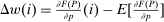 , where the expectation is with respect to P. With general Pareto weighting λ, (28) holds, but with elements of Δw redefined as
  .
.
 .
.
 and
and  in
in  , if each
  , then
  .
.
 .
.
 are highly correlated with those that attach high values to
  . Parameters of ϕ that control this correlation will be elevated.
 , which it knows will persist, relative to the Gumbel shock. However, this additional weight can be absorbed into redefined flow utilities generating an equivalent steady-state problem for the agent.