Monetary Policy, Redistribution, and Risk Premia
Abstract
We study the transmission of monetary policy through risk premia in a heterogeneous agent New Keynesian environment. Heterogeneity in households' marginal propensity to take risk (MPR) summarizes differences in portfolio choice on the margin. An unexpected reduction in the nominal interest rate redistributes to households with high MPRs, lowering risk premia and amplifying the stimulus to the real economy. Quantitatively, this mechanism rationalizes the role of news about future excess returns in driving the stock market response to monetary policy shocks and amplifies their real effects by 1.3–1.4 times.
1 Introduction
A growing literature finds that expansionary monetary policy lowers risk premia. This has been established for the equity premium in stock markets, the term premium in government bonds, and the external finance premium on risky corporate debt.1 The basic New Keynesian framework as in Woodford (2003) and Gali (2008) does not capture this aspect of monetary policy transmission. As noted by Kaplan and Violante (2018), this is equally true for emerging heterogeneous agent New Keynesian models in which heterogeneity in the marginal propensity to consume enriches the transmission mechanism but still cannot explain the associated movements in risk premia.
This paper demonstrates that a New Keynesian model with heterogeneous households differing instead in risk-bearing capacity can quantitatively rationalize the observed effects of policy on risk premia, amplifying the transmission to the real economy. An expansionary monetary policy shock lowers the risk premium on capital if it redistributes to households with a high marginal propensity to take risk (MPR), defined as the marginal propensity to save in capital relative to save overall. With heterogeneity in risk aversion, portfolio constraints, rules of thumb, background risk, or beliefs, high MPR households borrow in the bond market from low MPR households to hold leveraged positions in capital. By generating unexpected inflation, raising profit income relative to labor income, and raising the price of capital, an expansionary monetary policy shock redistributes to high MPR households, and thus lowers the market price of risk. In a calibration matching portfolio heterogeneity in the U.S. economy, this rationalizes the observed role of news about lower future excess returns in driving the increase in the stock market. The real stimulus is amplified by 1.3–1.4 times relative to an economy without heterogeneity in portfolios and MPRs.
Our baseline environment enriches a standard New Keynesian model with Epstein and Zin (1991) preferences and heterogeneity in risk aversion. Households consume, supply labor subject to adjustment costs in nominal wages, and choose a portfolio of nominal bonds and capital. Production is subject to aggregate TFP shocks. Monetary policy follows a Taylor (1993) rule. Heterogeneity in risk aversion generates heterogeneity in MPRs and exposures to a monetary policy shock. Epstein–Zin preferences imply that this heterogeneity is distinct from households' intertemporal elasticities of substitution. We first analytically characterize the effects of a monetary policy shock in a simple two-period version of this environment, providing an organizing framework for the quantitative analysis of the infinite horizon which follows.
An expansionary monetary policy shock lowers the risk premium by redistributing wealth to households with a high marginal propensity to save in capital relative to save overall, that is, a high MPR. Redistribution to high MPR households lowers the risk premium because of asset market clearing: if households on aggregate wish to increase their portfolio share in capital, its expected return must fall relative to that on bonds. An expansionary monetary policy shock redistributes across households by revaluing their initial balance sheets: it deflates nominal debt, raises the profits earned using capital, and raises the price of capital. More risk tolerant households hold leveraged positions in capital and have a higher MPR. Hence, an expansionary monetary policy shock will redistribute to these households and lower the risk premium.
The reduction in the risk premium amplifies the transmission of monetary policy to the real economy. Conditional on the real interest rate—which reflects the degree of nominal rigidity and the monetary policy rule—a decline in the required excess return on capital is associated with an increase in investment. The increase in investment crowds in consumption by raising household wealth. The stimulus to consumption and investment implies an increase in output overall.
These results are robust to heterogeneity beyond risk aversion. We consider a richer environment in which households may also face portfolio constraints or follow rules-of-thumb, may be subject to idiosyncratic background risk, and may have subjective beliefs regarding the value of capital. Because each of these still imply that households holding more levered positions in capital will be those with high MPRs, they continue to imply that expansionary monetary policy will lower the risk premium through redistribution, amplifying real transmission.
Accounting for the risk premium effects of monetary policy is important given empirical evidence implying that it may be a key component of the transmission mechanism. We refresh this point from Bernanke and Kuttner (2005) using the structural vector autoregression instrumental variables (SVAR-IV) approach in Gertler and Karadi (2015). We find that a monetary policy shock resulting in a roughly  reduction in the 1-year Treasury yield leads to a
  increase in the real S&P 500 return. Using a Campbell and Shiller (1988) decomposition and accounting for estimation uncertainty, 20–100% of this increase is driven by lower future excess returns, challenging existing New Keynesian frameworks where essentially all of the effect on the stock market operates through higher dividends or lower risk-free rates.
Extending the model to the infinite horizon, we investigate whether a calibration to the U.S. economy is capable of rationalizing these facts. We match the heterogeneity in wealth, labor income, and financial portfolios in the Survey of Consumer Finances, together disciplining the exposures to a monetary policy shock and MPRs. We use global solution methods to solve the model. To make the computational burden tractable, we model three groups of households: two groups corresponding to the small fraction with high wealth relative to labor income, but differing in their risk tolerance and thus portfolio share in capital, and one group corresponding to the large fraction holding little wealth relative to labor income. In the data, the high-wealth, high-leverage households are disproportionately those with private business wealth, while the high-wealth, low-leverage households are disproportionately retirees.
We find that the redistribution across households with heterogeneous MPRs can quantitatively explain the risk premium effects of an expansionary monetary policy shock. Notably, the redistribution relevant for this result is between wealthy households holding heterogeneous portfolios, rather than between the asset-poor and asset-rich. Using the same Campbell–Shiller decomposition as was used on the data, over 30% of the return on equity in our baseline parameterization arises from news about lower future excess returns, compared to 0% in a representative agent counterfactual. Consistent with the analytical results, the redistribution to high-MPR households is amplified with a more persistent shock, and thus larger debt deflation; higher stickiness, and thus a larger increase in profit income relative to labor income; or higher investment adjustment costs, and thus a larger increase in the price of capital.
Further consistent with the analytical results, the reduction in the risk premium through redistribution in turn amplifies the effect of policy on the real economy. In both our baseline and counterfactual representative agent economies, we study monetary policy shocks which deliver a  decline in the 1-year nominal yield on impact. Our model amplifies the response of quantities by 1.3–1.4 times: the peak investment, consumption, and output responses are
  ,
,  , and
, and  , while the counterparts in the representative agent economy are
  ,
,  , and
, and  .
.
Related Literature
Our paper contributes to the rapidly growing literature on heterogeneous agent New Keynesian (HANK) models by studying the transmission of monetary policy through risk premia. We build on Doepke and Schneider (2006) in our measurement of household portfolios, informing the heterogeneity in exposures to a monetary policy shock. The redistributive effects of monetary policy in our framework follow Auclert (2019). We demonstrate that it is the covariance of these exposures with MPRs rather than MPCs which matters for policy transmission through risk premia. Like Kaplan, Moll, and Violante (2018) and Luetticke (2021), we study an environment with bonds and capital. And like Alves, Kaplan, Moll, and Violante (2020), Auclert, Rognlie, and Straub (2020), and Melcangi and Sterk (2020) we study the effects of monetary policy shocks on asset prices. Unlike these models, in our framework assets differ in exposure to aggregate risk rather than in liquidity, allowing us to account for the important role of risk premia in driving the change in asset prices.
In doing so, we bring to the HANK literature many established insights from heterogeneous agent and intermediary-based asset pricing. The wealth distribution is a crucial determinant of the market price of risk as in other models with heterogeneous risk aversion (e.g., Garleanu and Panageas (2015)), segmented markets (e.g., He and Krishnamurthy (2013)), rules-of-thumb (e.g., Chien, Cole, and Lustig (2012)), background risk (e.g., Constantinides and Duffie (1996)), or heterogeneous beliefs (e.g., Geanakoplos (2009)).2 We build on this literature by focusing on the changes in wealth induced by a monetary policy shock in a production economy with nominal rigidities. In studying this question, we follow Alvarez, Atkeson, and Kehoe (2009) and Drechsler, Savov, and Schnabl (2018), who study the effects of monetary policy on risk premia in an exchange economy with segmented markets and in a model of banking, respectively.3 We instead study these effects operating through the revaluation of heterogeneous agents' balance sheets in a conventional New Keynesian setting.
Indeed, our paper most directly builds on prior work focused on risk premia in New Keynesian economies. We clarify the sense in which Bernanke, Gertler, and Gilchrist (1999) served as a seminal HANK model focused on heterogeneity in MPRs rather than MPCs.4 As we demonstrate, however, heterogeneity in MPRs need not rely on market segmentation, justifying its relevance even in markets that may not be intermediated by specialists. In relating movements in the risk premium to the real economy, we make use of the insight in Ilut and Schneider (2014), Caballero and Farhi (2018), and Caballero and Simsek (2020) that an increase in the risk premium will induce a recession if the safe interest rate does not sufficiently fall in response.5 We build especially on the latter two papers, as well as Brunnermeier and Sannikov (2012, 2016), in emphasizing the effects of heterogeneity in asset valuations on risk premia. Relative to these papers, we explore the importance of such heterogeneity for monetary transmission in a calibration to the U.S. economy.6
Like all of these papers, our analysis also provides a theoretical counterpart to the large empirical literature studying links between risky asset prices and real activity. Focusing first on stock prices, the evidence in support of the q-theory of investment has been mixed, and causal estimates of stock prices on consumption are complicated by the fact that they may simply be forecasting other determinants of consumption. Recently, Pflueger, Siriwardane, and Sunderam (2020) and Chodorow-Reich, Nenov, and Simsek (2021) have employed cross-sectional identification strategies to overcome these challenges, finding evidence in support of the cost-of-capital and consumption wealth mechanisms in our model. More broadly interpreting our model as studying the effect of monetary policy on risky claims on capital, there is substantial evidence that spreads on risky corporate debt predict real activity (e.g., Gilchrist and Zakrajsek (2012) and Lopez-Salido, Stein, and Zakrajsek (2017)).
Outline
In Section 2, we characterize our main insights in a two-period environment. In Section 3, we compare empirical evidence on the equity market response to monetary policy shocks to the quantitative predictions of our model enriched to the infinite horizon and calibrated to the U.S. economy. Finally, in Section 4 we conclude.
2 Analytical Insights in a Two-Period Environment
We first characterize our main conceptual insights in a two-period environment allowing us to obtain simple analytical results. Heterogeneity in risk aversion induces heterogeneity in household portfolios. An expansionary monetary policy shock lowers the risk premium on capital by redistributing to relatively risk tolerant households. A reduction in the risk premium amplifies the stimulus to investment, consumption, and output. These results are robust to heterogeneity in rules-of-thumb, portfolio constraints, background risk, or beliefs. More generally, they hold whenever households whose relative wealth rises upon a monetary easing have high propensities to save in capital relative to bonds, that is, high MPRs.
2.1 Environment
There are two periods, 0 and 1. To isolate the key mechanisms, we make a number of parametric assumptions that are relaxed later in the paper.
Households
 have Epstein–Zin preferences over consumption in each period
  and labor supply
  ,
,
 (1)
(1) , (dis)utility of labor
  , and Frisch elasticity θ. Labor in period 0 is not indexed by i because (as we describe below) households supply the same amount. In period 1, production only uses capital, and thus there is no labor supplied.
 and in capital
  subject to the resource constraints
 (2)
(2) (3)
(3) and
and  are its endowments in these same assets. The consumption good trades at
  units of the nominal unit of account (“dollars”) at t,7 the household earns a wage
  dollars in period 0, one dollar in bonds purchased at t yields
  dollars at
  , and one unit of capital purchased for
  dollars at t yields a dividend
  plus
plus  dollars at
  . Capital fully depreciates after period 1 (
 ).
).Supply-Side
 (4)
(4) units of labor and rents
  units of capital from households to produce the final good with TFP of one. It also uses
  units of the consumption good to produce
  new capital sold to households, where
  indexes adjustment costs and it takes
  as given. The producer thus earns
 (5)
(5) units of capital and has TFP
  , so it earns
 (6)
(6) (7)
(7)Policy
 by committing to
  , eliminating inflation risk in the nominal bond,
 , where
  is the shock of interest. It follows that the real interest rate between periods 0 and 1 is
Market Clearing
 (9)
(9) (10)
(10) (11)
(11) (12)
(12)Equilibrium
Given the state variables  and a stochastic process for
  in (7), the definition of equilibrium is then standard.
Definition 1.An equilibrium is a set of prices and policies such that: (i) each household i chooses  to maximize (1) subject to (2)–(3), (ii) wages are rigid as in (4), (iii) the representative producer chooses
  to maximize profits (5) and earns profits (6), (iv) the government sets
  according to
  and (8), and (v) the goods, capital, and bond markets clear according to (9)–(12).
We now characterize the comparative statics of this economy with respect to a monetary policy shock  in a sequence of three main propositions. Each result builds on the last, and each makes use of only a few equilibrium conditions.
2.2 Monetary Policy, Redistribution, and the Risk Premium
We first provide a general result characterizing the effect of a monetary policy shock on the expected excess return on capital.


 denote the gross real returns on capital

 is given by
 (13)
(13) (14)
(14)Simply by aggregating (14) and making use of the asset market clearing conditions (10) and (12), we obtain the first result of the paper, the proof of which (along with all other proofs) is in Appendix A in the Online Supplementary Material (Kekre and Lenel (2022)).
Proposition 1.The risk premium on capital is


 (15)
(15)Hence, a monetary policy shock affects the risk premium if it redistributes across households with heterogeneous desired portfolios. If monetary policy does not redistribute ( for all i) or households have identical desired portfolios (
 for all i), there is no effect on the risk premium. Away from this case, redistributing wealth to households with relatively high desired portfolios in capital lowers the risk premium. Intuitively, such redistribution raises the relative demand for capital, lowering the required excess return to clear asset markets.
2.3 Risk Premium and the Real Economy
We now characterize why a change in the risk premium is relevant for the real economy.
 (16)
(16)
 (17)
(17)Proposition 2.The change in investment in response to a monetary shock is
 (18)
(18) in response to a monetary shock is

 in response to a monetary shock is
 (19)
(19)Thus, conditional on the real interest rate, a decline in the risk premium is associated with an increase in investment. The increase in investment stimulates aggregate demand, and thus production. Consumption rises both because of the increase in the value of capital holdings and because of the rise in disposable income induced by higher production. This feeds back to further stimulate aggregate demand, and thus production.10 These results apply to the case of a monetary policy shock the broader insights of Caballero and Simsek (2020) linking risk premia and the real economy.
2.4 Monetary Transmission via the Risk Premium
We now sign the transmission of a monetary policy shock via the risk premium.
 (20)
(20) , the change in its wealth share is in turn
 (21)
(21)Hence, in this setting there are three channels through which wealth is redistributed on impact of a monetary policy shock: via inflation (which redistributes toward nominal borrowers) or via an increase in profits or the price of capital (which redistribute toward those with a disproportionate claim on capital). These heterogeneous exposures to a monetary shock have been previously exposited in the HANK literature, as by Auclert (2019). Propositions 1 and 2 imply that it is their covariance with desired portfolio shares that matters for transmission through risk premia.
When agents' initial endowments are consistent with their desired portfolios in period 0—as would be the case in the steady-state of an infinite horizon model—and they start with same initial levels of wealth, we can sharply sign these effects.
Proposition 3.Suppose agents differ in risk aversion  ; their initial endowments are consistent with their desired portfolio in period 0 (
 ); and they have the same initial levels of wealth. Then:
- a cut in the nominal interest rate lowers the risk premium, and
- the resulting stimulus to investment, consumption, and output are larger than a representative agent economy starting from the same aggregate allocation.
Intuitively, relatively risk tolerant agents finance levered positions in capital by borrowing in nominal bonds.11 A cut in the nominal interest rate generates inflation, an increase in profits, and an increase in the price of capital, redistributing wealth to these agents. Proposition 1 implies that this lowers the risk premium. At least given a conventional Taylor rule, the endogenous response of the real interest rate is not sufficiently strong to overturn the amplification characterized in Proposition 2.
2.5 Other Sources of Heterogeneity
The preceding results do not rely on heterogeneity in risk aversion alone; they also apply when there is heterogeneity in portfolios arising from other primitives.
Binding Constraints or Rules-of-Thumb

 in particular, this means the household cannot participate in the capital market. Such constraints are consistent with prior asset pricing models with segmented markets or rules-of-thumb as well as macroeconomic models of the financial accelerator.
Background Risk
 in period 1, modeled as a multiplicative change in the efficiency units of capital.
  is iid across households and independent of the aggregate TFP shock
  , and
, and  controls the degree of background risk according to

Subjective Beliefs

 are “pessimists” and households with
  are “optimists.”
We can then prove the following.
Proposition 4.Suppose households differ in risk aversion  , being constrained and (among those that are) constraints
  , background risk
  , and beliefs
  . Further suppose that their endowments are identical to their choices in period 0 and they are otherwise identical. Then we obtain the same results as in Proposition 3.
 , background risk
  , and pessimism
  , and rising in the leverage constraint or rule-of-thumb
  (if applicable). Regardless of these underlying drivers, so long as households enter period 0 with endowments reflecting these same portfolios, it will be the case that an expansionary monetary policy shock redistributes to those wishing to hold relatively more capital. Thus, an expansionary shock lowers the risk premium, amplifying the stimulus to the real economy.
2.6 Exposures and the Marginal Propensity to Take Risk
The robustness of these results derives from the tight link between households' exposures to a monetary policy shock and their marginal portfolio choices given a dollar of income. In a more general environment, we now demonstrate that it is the covariance between the two which governs the effects of such a shock on the risk premium.
Consider how a household's optimal portfolio changes with an additional dollar of income. Let the capital, bond, and total savings policy functions solving each household's micro-level optimization problem be given by  ,
,  , and
, and  , respectively. Their arguments are the household's wealth
  and all other aggregates that the household takes as given, such as the real interest rate
  and price of capital
  . Then we have the following.
Definition 2.Household i's marginal propensity to take risk (MPR) is

In the environment studied in the prior subsections, households' marginal and equilibrium portfolios are identical ( ). This is no longer the case if households have a nonunitary elasticity of intertemporal substitution or supply labor in period 1.12 We can still obtain analytical results in this more general environment, however, by studying the limit as aggregate risk falls to zero. In doing so, we apply techniques developed by Devereux and Sutherland (2011) in the context of open-economy macroeconomics to the present environment and our particular statistics of interest.13 Letting variables with bars denote values at the point of approximation without aggregate risk, and returning to the case without portfolio constraints, rules-of-thumb, background risk, and belief differences for simplicity, we obtain the following.
Proposition 5.At the limit of zero aggregate risk, i's portfolio share in capital is
 (22)
(22) (23)
(23) (24)
(24)This proposition naturally generalizes (14). It remains that a household's portfolio share in capital and its MPR are higher the less risk averse it is relative to other households in the economy.14 Nonetheless, the portfolio share and MPR are no longer the same: a household's portfolio share in capital depends not only on risk aversion but also its motive to hedge labor income also subject to TFP shocks, captured by the last term in (22). This hedging motive is irrelevant on the margin.
The distinction between portfolios and MPRs is useful in clarifying their roles in a generalization of Proposition 1, our final analytical result of the paper. Approximating households' optimal portfolio choice (13) and the asset market clearing conditions (10) and (12) around the point with zero aggregate risk, and denoting with hats log/level deviations from this point, we obtain the following.
Proposition 6.Up to third order in the perturbation parameters  ,
,
 (25)
(25)Hence, a monetary policy shock will lower the risk premium if it redistributes wealth to households with relatively high MPRs. This decouples and clarifies the respective role of portfolios and MPRs. Portfolios—more precisely, those which households enter the period with—govern how wealth redistributes on impact of a monetary policy shock, and are contained in  . MPRs govern how agents allocate the change in wealth on the margin. We will thus focus on heterogeneity in both portfolios and MPRs in our quantitative results, to which we now turn.
3 Quantitative Relevance in the Infinite Horizon
We first revisit the empirical evidence on the equity premium response to monetary policy shocks, which poses a challenge to workhorse models where risk premia barely move. We then calibrate our model to match standard “macro” moments as well as novel “micro” moments from the Survey of Consumer Finances, which discipline the cross-sectional heterogeneity in MPRs and exposures to monetary policy. In response to an unexpected monetary easing in our model economy, wealth endogenously redistributes to relatively high MPR households, rationalizing the equity premium response found in the data and amplifying the stimulus in real activity.
3.1 Empirical Effects of Monetary Policy Shocks in U.S. Data
The effects of an unexpected shock to monetary policy have been the subject of a large literature in empirical macroeconomics. In response to an unexpected loosening, the price level rises and production expands, consistent with workhorse New Keynesian models. But, as found in Bernanke and Kuttner (2005) and a number of subsequent papers using asset pricing data, the evidence further suggests that risk premia fall.15,16
We refresh the findings in Bernanke and Kuttner (2005) using the structural vector autoregression instrumental variables (SVAR-IV) approach in Gertler and Karadi (2015). Using monthly data from July 1979 through June 2012, we first run a six-variable, six-lag VAR using the 1-year Treasury yield, CPI, industrial production, 1-month T-bill return relative to the change in CPI, S&P 500 return relative to the 1-month T-bill, and smoothed dividend-price ratio on the S&P 500.17,18 Over January 1991 through June 2012, we then instrument the residuals in the 1-year Treasury yield (the monetary policy indicator) with an external instrument: policy surprises constructed using the current Fed Funds futures contract on FOMC days aggregated to the month level from Gertler and Karadi (2015). The identification assumptions are that the exogenous variation in the monetary policy indicator in the VAR are due to the structural monetary shock and that the instrument is correlated with this structural shock but not the five others. With a first-stage F statistic of 14.4, this instrument is strong according to the threshold of Stock, Wright, and Yogo (2002).
We then plot the impulse responses to a negative monetary policy shock using this instrument in Figure 1. Since the structural monetary policy shock is not observed, its magnitude should be interpreted through the lens of the approximately  decrease in the 1-year yield on impact. Consistent with the wider literature, industrial production and the price level rise, and the real interest rate falls. Excess returns rise by 1.9pp on impact; given the comparatively tiny decline in the real interest rate, this means the real return on the stock market is also approximately 1.9pp. Notably, excess returns are small and negative in the months which follow, consistent with a decline in the equity premium and the fall in the dividend/price ratio.

Effects of 1 SD monetary shock. Notes: 90% confidence interval at each horizon is computed using the wild bootstrap with 10,000 iterations, following Mertens and Ravn (2013) and Gertler and Karadi (2015).
 (26)
(26) and
and  is the steady-state dividend yield. Using the SVAR-IV to compute the revised expectations in real rates and excess returns given the monetary shock, we obtain the decomposition in Table I.19 1.1pp (59%) of the initial return on the stock market is due to news about lower future excess returns, 0.1pp (8%) is due to news about lower future risk-free rates, and 0.6pp (33%) is due to news about higher dividend growth. Accounting for estimation uncertainty, at least 19% and potentially all of the return on the stock market is due to news about lower future excess returns, validating the original message from Bernanke and Kuttner (2005).
|
pp |
As Share of Effect on Real Stock Return |
|
|---|---|---|
|
Real stock return |
1.92 |
|
|
|
||
|
Dividend growth news |
0.64 |
33% |
|
|
|
|
|
− Future real rate news |
0.15 |
8% |
|
|
|
|
|
− Future excess return news |
1.13 |
59% |
|
|
|


-
Note: Decomposition in (26) uses
 following Campbell and Ammer (1993). 90% confidence interval in brackets is computed using the wild bootstrap with 10,000 iterations, following Mertens and Ravn (2013) and Gertler and Karadi (2015).
The important role of the risk premium in explaining the return on the stock market is robust to details of the estimation approach. In Appendix B.1, we change the number of lags used in the VAR; change the sample periods over which the VAR and/or first-stage is estimated; add variables to the VAR; and use an alternative instrument for the monetary policy shock. Across these cases, we confirm the message of the baseline estimates above: in response to a monetary policy shock that reduces the 1-year Treasury yield by approximately  , real stock returns rise by 1.5–3.1pp, and news about future excess returns explains 35%–85% of this increase.
The dimensionality reduction offered by a VAR enables us to generate the long-horizon forecasts needed for the Campbell–Shiller decomposition, unlike a local projection. As noted by Stock and Watson (2018), we can test the assumption of invertibility implicit in the SVAR-IV both by assessing whether lagged values of the instrument have forecasting power when included in the VAR and by comparing the estimated impulse responses to those obtained using a local projection with instrumental variables (LP-IV). We show in Appendix B.1 that both of these tests fail to reject the null hypothesis that invertibility in our application is satisfied.20
Finally, augmenting our VAR with cross-sectional data corroborates the redistributive mechanism through which our model rationalizes the risk premium response to a monetary shock. In Appendix B.1, we construct two measures of the relative wealth of agents relatively more exposed to the stock market: a total return index of high beta hedge funds relative to low beta hedge funds, and an analogous index for mutual funds. These measure the relative wealth of a household continually (re)invested in high beta funds relative to low beta funds. On impact of a monetary easing, we find that the relative return of high beta funds rises on impact and then falls thereafter. This is consistent with the wealth share of relatively risk tolerant investors rising, since risk sharing calls for the wealth of risk tolerant investors to load more on the return on capital, that is, to have a higher beta.
Objectives in the Remainder of Paper
The rest of the paper enriches the model from Section 2 and studies a calibration to the U.S. economy matching micro evidence on portfolio heterogeneity and conventional macro moments on asset prices and business cycles. We first ask whether redistribution in such an environment can quantitatively rationalize the estimated stock market response to a monetary policy shock. We then use the model to quantify the implications for the real economy.
3.2 Infinite Horizon Environment
We first outline the environment, building on that from Section 2.1. We describe the main changes here and present the complete environment in Appendix C.
3.2.1 Household Preferences and Constraints
To ensure a stationary wealth distribution despite permanent differences in risk aversion, we assume a perpetual youth structure in which each household dies at rate ξ and has no bequest motive. This implies an underlying wealth distribution among households having a particular coefficient of relative risk aversion  . Appendix C proves the existence of a representative household at each
  .21
.21
 (27)
(27) (28)
(28) reflects the wealth of households of type i at
  who were also alive at t, relative to the average household of type i at
  . It is characterized in Appendix C.
 (29)
(29) controls the magnitude of adjustment costs,
  is the economy-wide wage bill, and
  in the reference wage is an adjustment for rare disasters described below. These adjustment costs are not indexed by i because there is a common wage for each variety supplied by households, as described below. We further assume these costs are paid to the government and rebated back to households so that they only affect the allocation via the dynamics of wages.
 (30)
(30) is productivity, discussed below. Such a constraint captures components of capital which households hold for reasons beyond financial returns, such as housing.
3.2.2 Supply-Side
 and
and  to maximize the utilitarian social welfare of union members given the allocation rule
 (31)
(31) . A representative labor packer purchases varieties and combines them to produce a CES aggregate with elasticity of substitution ϵ,
 (32)
(32) , earning
 (33)
(33)3.2.3 Aggregate Productivity
 follows a unit root process
 (34)
(34) is an iid shock from a Normal distribution with mean zero and standard deviation
  ,
,  is a rare disaster equal to zero with probability
  and
and  with probability
  , and
, and  follows an AR(1) process
 (35)
(35) is an iid shock from a Normal distribution with mean zero and standard deviation
  . Following Barro (2006), Gourio (2012), and Wachter (2013), we introduce the disaster with time-varying probability to help match the level of the equity premium and volatility of returns.22 So that the dynamics upon a rare disaster are well behaved, we assume that the disaster destroys capital and reduces the reference wage in households' wage adjustment costs in proportion to the decline in productivity. The first assumption implies that aggregate output is
 (36)
(36)3.2.4 Monetary and Fiscal Policy
 (37)
(37) (38)
(38) is an iid shock from a Normal distribution with mean zero and standard deviation
  .
.Fiscal policy is characterized by three elements. First, the government subsidizes workers' labor income at a constant rate  rebated back to each household, eliminating the average wage markup in the usual way. Second, the government participates in the bond market financed by lump-sum taxes in which household i pays a share
  . Given the latter assumption (and that households face no constraints in the bond market) the government bond position has no effect on the equilibrium allocation, so we assume it is a constant real value relative to productivity:
  . Its only purpose is to make measured portfolios in model and data comparable. Third, the government collects the wealth of dying households and endows it to newborn households. We describe the rule employed when doing so in the next subsection.
3.2.5 Equilibrium and Model Solution
The definition of equilibrium naturally generalizes Definition 1.
We solve the model globally using numerical methods. Given this, we limit the heterogeneity across households to make the computation tractable. We divide the continuum of households into three groups  within which households have identical preferences. The index i now refers to the representative household of each group. The fraction of households belonging to group i is denoted
  , where
  .
.
 and nominal variables by
  . In the transformed economy, we obtain a recursive representation of the equilibrium in which the aggregate state in period t is given by the monetary policy state variable
  , disaster probability
  , scaled aggregate capital
  , scaled prior period's real wage
  , and wealth shares
  of any two groups. Assuming that the government endows newborn households of each group with a share
  of dying households' wealth, these wealth shares follow
 (39)
(39)We solve the model using sparse grids as described in Judd, Maliar, Maliar, and Valero (2014). When forming expectations, we use Gauss–Hermite quadrature and interpolate with Chebyshev polynomials for states off the grid. The stochastic equilibrium is determined through backward iteration, while dampening the updating of asset prices and individuals' expectations over the dynamics of the aggregate states. The code is written in Fortran and parallelized using OpenMP, so that convergence can be achieved in a few minutes on a standard desktop computer.
3.3 Parameterization, First Moments, and Second Moments
We now parameterize the model to match micro moments informing the heterogeneity across groups as well as macro moments regarding the business cycle and asset prices.
3.3.1 Micro: The Distribution of Wealth, Labor Income, and Portfolios
We seek to match the distribution of wealth, labor income, and financial portfolios in U.S. data, giving us confidence in the model's MPRs and exposures to a monetary shock. We proceed in three steps with the 2016 Survey of Consumer Finances (SCF).
First, we decompose each household's wealth ( ) into claims on the economy's capital stock (
 , in positive net supply) and nominal claims (
 , in zero net supply accounting for the government and rest of the world). We describe this procedure in detail in Appendix B.2 and provide a broad overview here. We first add estimates of defined benefit pension wealth for each household since this is the major component of household net worth that is excluded from the SCF.23 We then proceed by line item to allocate how much household wealth is held in nominal claims versus claims on capital.24 In the same spirit as Doepke and Schneider (2006), the key step in doing this is to account for the implicit leverage households have on capital through publicly-traded and privately-held businesses. The aggregate leverage implicit in these equity claims must be consistent with that of the business sectors in the Financial Accounts of the United States. We parameterize the dispersion in leverage in these claims to match evidence on the dispersion in households' expected rates of return.
Second, we stratify households by their wealth to labor income  and capital portfolio share
  , defining our three groups. We sort households on these variables based on Proposition 5, which demonstrated that the capital portfolio share is informative about households' risk aversion, and thus MPR, only after properly accounting for their nontraded exposure to aggregate risk through labor income.25 Group a corresponds to households with high wealth to labor income and a high capital portfolio share, group b corresponds to households with high wealth to labor income but a low capital portfolio share, and group c corresponds to households with low wealth to labor income. We define “high” wealth to labor income as households above the 60th percentile of this measure, and a “high” capital portfolio share as households above the 90th percentile of this measure.26
Third, we summarize the labor income, wealth, and financial portfolios of these three groups, provided in Table II. Group a households earn 3% of labor income, hold 18% of wealth, and have an aggregate capital portfolio share of 2.0. Group b households earn only 14% of labor income, hold 58% of wealth, and have an aggregate capital portfolio share of 0.5. Group c households earn 83% of labor income, hold only 23% of wealth, and have an aggregate capital portfolio share of 1.1. To better understand the nature of households in each group, in Table III we first project an indicator for the household having private business wealth on households' group indicator. Households in group a are especially more likely to have private business wealth. We then project an indicator for the household head being older than 54 and out of the labor force, together capturing a retired household head, on households' group indicator. Households in group b are especially more likely to be retired.
|
|
|||
|
|
|
||
|
|
|
Group a |
|
|
Share households: 4% |
|||
|
∑i∈aWℓi/∑iWℓi: 3% |
Group c |
||
|
∑i∈aAi/∑iAi: 18% |
Share households: 60% |
||
|
∑i∈aQki/∑i∈aAi: 2.0 |
∑i∈cWℓi/∑iWℓi: 83% |
||
|
|
Group b |
∑i∈cAi/∑iAi: 23% |
|
|
Share households: 36% |
∑i∈cQki/∑i∈cAi: 1.1 |
||
|
∑i∈bWℓi/∑iWℓi: 14% |
|||
|
∑i∈bAi/∑iAi: 58% |
|||
|
∑i∈bQki/∑i∈bAi: 0.5 |
|||


- Note: Observations are weighted by SCF sample weights.
|
1{hbusi = 1} |
1{agei > 54,lfi = 0} |
|
|---|---|---|
|
1{i ∈ a} |
0.37 |
0.37 |
|
(0.03) |
(0.03) |
|
|
1{i ∈ b} |
0.05 |
0.55 |
|
(0.01) |
(0.01) |
|
|
Observations |
6,229 |
6,229 |
|
Adj R2 |
0.05 |
0.37 |
- Note: observations are weighted by SCF sample weights and standard errors adjust for imputation and sampling variability following Pence (2015). Each specification includes a constant term (not shown), capturing the baseline probability of holding private business wealth or being retired among households in group c.
In Appendix B.2, we apply the exact same approach as above to stratify households in 2007 using the 2007–2009 SCF panel. We then exploit the panel structure of this survey to follow households through 2009. Among other findings, we document that households' portfolio share in capital are very persistent across these 2 years, both at the group and individual levels. This validates our calibration approach of matching the cross-sectional data using permanent differences in households' risk preferences.
3.3.2 Macro: Business Cycle Dynamics and Asset Prices
We also calibrate the model to match standard macro moments regarding the business cycle and asset prices. In terms of the business cycle, we use NIPA data on consumption of nondurables and services as well as investment in durables and capital, together with the time series of the working age population from the BLS, to estimate the volatilities of quarterly per capita growth rates in those series over Q3 1979 to Q2 2012 (consistent with our sample period for the VAR). In terms of asset prices, we use the data from CRSP described earlier to estimate the annualized average real interest rate and excess return on the S&P 500 over July 1979–June 2012. We further estimate the second moments of expected returns using our VAR. We compute analogous moments in our model assuming that an equity claim (with return  ) is a levered claim to capital with a debt to equity ratio of 0.5.27
3.3.3 Parameterization
A model period corresponds to one quarter. After setting a subset of parameters in accordance with the literature, we calibrate the remaining parameters to be consistent with the macro and micro moments described above. All stochastic properties of the model are estimated using a simulation where no disasters are realized in the sample.28
Externally Set Parameters
A subset of model parameters summarized in Table IV are set externally. Among the model's preference parameters, we set ψ to 0.8. We note that this parameter controls both the intertemporal elasticity of substitution in consumption as well as the complementarity between consumption and labor. A value less than one is consistent with evidence on the consumption responses to changes in interest rates as well as consumption-labor complementarity.29 The Frisch elasticity of labor supply is set to  , roughly consistent with the micro evidence for aggregate hours surveyed in Chetty, Guren, Manoli, and Weber (2011). The three types have measure
  ,
,  , and
, and  and the labor allocation rule features
  ,
,  , and
, and  , consistent with Table II. Households die with probability
  , implying an expected horizon of 25 years, consistent with households transitioning across groups through the life cycle.
|
Description |
Value |
Notes |
|
|---|---|---|---|
|
ψ |
IES |
0.8 |
|
|
θ |
Frisch elasticity |
1 |
|
|
λa |
measure of a households |
4% |
population in SCF |
|
λb |
measure of b households |
36% |
population in SCF |
|
ϕa |
labor a households |
3%/λa |
labor income in SCF |
|
ϕb |
labor b households |
14%/λb |
labor income in SCF |
|
ξ |
death probability |
1% |
|
|
α |
1—labor share |
0.33 |
|
|
δ |
depreciation rate |
2.5% |
|
|
ϵ |
elast. of subs. across workers |
10 |
|
|
χW |
Rotemberg wage adj costs |
150 |
|
|
|
disaster probability |
0.45% |
|
|
|
disaster shock |
−15% |
|
|
ϕ |
Taylor coeff. on inflation |
1.5 |
|
|
σm |
std. dev. MP shock |
0.25%/4 |
|
|
ρm |
persistence MP shock |
0 |
|
|
λaνa |
a share of taxes to finance −Bg |
18% |
wealth in SCF |
|
λcνc |
c share of taxes to finance −Bg |
23% |
wealth in SCF |


On the production side, we choose standard values of  for the capital share of production and
  for the quarterly depreciation rate. We set
  so that, accounting for Jensen's inequality and the calibrated volatility and persistence
  and
and  below, the average disaster probability
  . This follows Barro (2006) and implies that a disaster shock is expected to occur every 50 years. The depth of the disaster is set to
  , consistent with the estimates of Nakamura, Steinsson, Barro, and Ursua (2013) who account for the recovery after a disaster. We choose an elasticity of substitution across worker varieties
  and Rotemberg wage adjustment costs of
  , together implying a Calvo (1983)-equivalent frequency of wage adjustment between 4 and 5 quarters, consistent with the evidence in Grigsby, Hurst, and Yildirmaz (2021).
Finally, in terms of policy, we set the Taylor coefficient on inflation to the standard value  . Monetary policy shocks have a standard deviation of
  with zero persistence. The share of lump-sum taxes financing government debt paid by group i (
 ) is equal to their wealth share in Table II.
Calibrated Parameters
We calibrate the remaining parameters to target the macro and micro moments described above. Table V reports in each line a parameter choice and moment in model and data that this parameter is closely linked to.
|
Description |
Value |
Moment |
Target |
Model |
|
|---|---|---|---|---|---|
|
σz |
std. dev. prod. |
0.55% |
σ(Δlogc) |
0.5% |
0.6% |
|
χx |
capital adj cost |
3.5 |
σ(Δlogx) |
2.1% |
2.0% |
|
β |
discount factor |
0.98 |
4r+1 |
1.3% |
1.5% |
|
γb |
RRA b |
25.5 |
|
7.3% |
7.0% |
|
σp |
std. dev. log dis. prob. |
0.47 |
|
2.2% |
2.2% |
|
ρp |
persist. log dis. prob. |
0.8 |
|
0.79 |
0.75 |
|
γa |
RRA a |
10 |
qka/aa |
2.0 |
2.3 |
|
|
lower bound ki |
10 |
qkc/ac |
1.1 |
0.9 |
|
|
newborn endowment a |
0% |
λaaa/∑iλiai |
18% |
21% |
|
|
newborn endowment c |
−0.25% |
λcac/∑iλiai |
23% |
23% |
|
bg |
real value govt. bonds |
−2.7 |
−∑iλibi/∑iλiai |
−10% |
−10% |


-
Note: Targeted business cycle moments are from Q3/79–Q2/12 NIPA and targeted asset pricing moments are from 7/79–6/12 data underlying the VAR. The model assumes a debt/equity ratio of 0.5 on a stock market claim. The first and second moments in the model are estimated over 50,000 quarters after a burn-in period of 5,000 quarters, with no disaster realizations in sample. The disutilities of labor
 are jointly set to
  so that the average labor wedge is zero for each group and
  , where the latter is a convenient normalization. The Taylor rule intercept
  is set to 0.3% to target zero average inflation.
We first match the first and second moments of quantities and returns. The standard deviation of the productivity shock  is set to 0.55% to match quarterly consumption growth volatility of 0.5%. The capital adjustment cost is set to
  to target the volatility of investment growth. Due to the precautionary savings motive,
  is high enough to match the low annualized real rate observed in the data. We set
  to target the annualized excess return on equity. The standard deviation
  and persistence
  in the disaster probability process target the standard deviation and autocorrelation of the annualized expected real rate from our VAR.
We next match the micro heterogeneity in portfolios and wealth. We set  to target a households' capital portfolio share.
  and
and  are difficult to separately calibrate: the relatively high ratio of labor income to wealth among group c households means that they would endogenously choose to hedge this exposure to productivity shocks by holding a lower position in capital, consistent with Proposition 5, and are thus more likely to be constrained by (30). We set
  equal to the (population-weighted) harmonic mean of
  and
and  and calibrate
  to target the capital portfolio share of c households in the data.30 The initial endowments of newborns are chosen to target the measured wealth shares of the three groups. Matching these wealth shares requires that only b households receive a positive endowment when born.31
Finally, we set  so that the aggregate bond position of households relative to total wealth is 10%, as implied by Table II. We set the disutilities of labor so that the average labor wedge is zero for each group and
  , the latter a convenient normalization. We set the Taylor rule intercept
  so that average inflation is zero.
3.3.4 Untargeted Moments
Table VI reports the values of several untargeted moments and their empirical counterparts. In terms of macro moments, the model closely matches the quarterly volatilities of output growth, employment growth, and the smoothed dividend price ratio.32,33 Related to the latter, the model generates a quarterly volatility of annualized expected excess equity returns of 2.8%, which accounts for more than half of the volatility estimated in the data by the studies surveyed in Duarte and Rosa (2015).
|
Moment |
Data |
Model |
|---|---|---|
|
σ(Δlogy) |
0.8% |
0.9% |
|
σ(Δlogℓ) |
0.8% |
0.8% |
|
σ(d/p) |
0.2% |
0.2% |
|
∑iλimpri |
≈ 0.2 |
0.3 |
|
mpra |
1.9 |
|
|
mprb |
0.7 |
|
|
mprc |
0.0 |
|
|
∑iλimpci |
≈ 0.2 |
0.02 |
|
mpca |
0.02 |
|
|
mpcb |
0.02 |
|
|
mpcc |
0.02 |
- Note: See notes accompanying Table V on construction of moments in data and model.
Turning to micro moments, we first consider MPRs. The model generates heterogeneity in quarterly MPRs consistent with Proposition 5 in the analytical results. Group a households are the most risk tolerant and have the highest MPR, borrowing $0.9 for every $1 of marginal net worth to invest in capital. Group b and c households have higher levels of risk aversion and correspondingly lower MPRs. As noted above, group c households have a higher ratio of labor income to wealth, and thus are endogenously constrained by (30). Hence, on the margin their average MPR is zero.
Quasiexperimental evidence is consistent with the MPRs in our calibration. Weighting by the fraction of households, the average MPR in our model is 0.3. Using data on Norwegian lottery winners, Fagereng, Holm, and Natvik (2021) estimate an average marginal propensity to save in risky assets relative to save overall of 0.14.34 Using data on Swedish lottery winners, Briggs, Cesarini, Lindqvist, and Ostling (2015) estimate an analogous ratio of 0.15.35 These imply an MPR of roughly 0.2 after accounting for reasonable estimates of the leverage of firms in which households invest.36 MPRs further rise with wealth per household in our calibration—recalling that wealth per household is highest among a households and then b households—consistent with evidence from these studies.37 While the range in estimated MPRs in these studies is smaller than that in our model, estimated MPRs based on lotteries may underestimate the relevant statistic for households in groups a and b of our model. As lottery winnings are paid out as cash or riskless deposits, the estimated MPR may understate the MPR in response to dividends or capital gains, more relevant for the balance sheet revaluation among the wealthy (a and b households) emphasized in this paper.38 Among owners of private businesses, overrepresented in these households, the estimated MPR may particularly understate their true MPR because investment in private businesses is not included in the definition of (traded) risky assets.
The model's heterogeneity in MPRs contrasts with its implied MPCs, which are essentially identical across agents. This is an intentional implication of our model environment, which features no idiosyncratic labor income risk nor heterogeneity in discount factors, allowing us to focus on the consequences of heterogeneity in portfolio choice alone. Unsurprisingly, the model further generates an average quarterly MPC that is an order of magnitude lower than typically estimated in the data. We expect that adding additional features to our model that raise the average MPC would only amplify the real consequences of movements in the risk premium.39
We finally note that, consistent with our analytical results, it is the exposures and MPRs in our calibration that are essential for the effects of a monetary shock—not the precise microfoundation. In Appendix D.3, we consider an alternative environment in which households have identical risk aversion but are exposed to heterogeneous amounts of idiosyncratic risk in their return on capital, as in the environment with background risk described in Section 2.5 and the broader literature on entrepreneurship in macroeconomic models. To match the same data on portfolios, a households are calibrated to be exposed to less idiosyncratic risk than other agents; equivalently, their risk-adjusted returns are highest. The resulting MPRs are very similar to the baseline model, and the quantitative results which follow are robust.
3.4 Impulse Responses to a Monetary Policy Shock
We now simulate the effects of a negative shock to the nominal interest rate. We demonstrate that our model can rationalize the stock market responses to a monetary policy shock in the data. The effects of monetary policy on the risk premium on capital amplify the transmission to the real economy by 1.3–1.4 times.
3.4.1 Model versus RANK
Figures 2, 3, and 4 compare the impulse responses to those in a counterfactual representative agent New Keynesian (RANK) economy. In the latter, we set  for all groups, equal to the wealth-weighted harmonic mean of risk aversion in the model.

Expected returns after negative monetary policy shock. Notes: Series are quarterly (nonannualized) measures, except for the 1-year nominal bond yield Δi1y. Impulse responses are the average response (relative to no shock) starting at 1,000 different points drawn from the ergodic distribution of the state space, itself approximated using a sample path over 50,000 quarters after a burn-in period of 5,000 quarters. bp denotes basis points (0.01%).

Redistribution after negative monetary policy shock. Notes: See notes accompanying Figure 2 on construction of impulse responses.

Quantities after negative monetary policy shock. Notes: See the notes accompanying Figure 2 on construction of impulse responses.
We choose the shock  in our model to generate a
  reduction in the 1-year nominal yield, consistent with Section 3.1. We obtain this yield by computing, in each state, the price that each household would pay for a 1-year nominal bond. We then set the price to that of the highest-valuation household. Importantly, we recalibrate
  in the RANK economy to match this same decline in the 1-year yield.
Figure 2 summarizes the effect of the monetary policy shock on expected returns. The first panel reports the change in the yield on the 1-year nominal bond. The second and third panels depict the resulting change in the expected real interest rate and the expected excess returns on capital. The latter is clear: the risk premium declines substantially and persistently in the model, unlike RANK. The former is more nuanced: the expected real interest rate initially declines by more relative to RANK, but in the subsequent quarters exceeds that in RANK. This is because we need to simulate a more negative  in the model to match the same decline in the 1-year Treasury, since monetary policy endogenously tightens in subsequent quarters in response to the stimulus from lower risk premia. For this reason, the results which follow are similar if we calibrate the shock in RANK to minimize the absolute value difference between the expected real interest rate path versus the model. Following Proposition 2, we can thus interpret differences in the macro dynamics between the model and RANK as arising from the differing risk premium responses.
Figure 3 demonstrates that redistribution drives the decline in the risk premium in our model. The first panel of the first row demonstrates that realized excess returns on capital are substantially positive on impact, followed by small negative returns in the quarters which follow—consistent with the initial decline in expected excess returns and the empirical pattern estimated in Figure 1. The positive excess return on impact follows from each of the channels characterized in Section 2.4: unexpected inflation, which lowers the realized real interest rate,40 shown in the third panel; a higher price of capital, shown in the first panel of the second row; and higher short-run profits due to lower real wages and higher employment in this sticky wage environment, shown in the second and third panels of this row. Together these forces redistribute to the high MPR a households who hold levered claims on capital, evident from their financial wealth share shown in the second panel of the first row. The persistence in their wealth share drives the persistent decline in expected excess returns.
Figure 4 examines the consequences for policy transmission to the real economy. The impact effects on investment, consumption, and output are 1.3–1.4 times larger versus the RANK economy. Moreover, the stimulus in our model remains persistently higher than the RANK economy despite the endogenous tightening of monetary policy in the model because the risk premium falls by more than the risk-free rate rises. These patterns are consistent with our discussion of Proposition 2.
Quantitatively, the price and quantity effects of the monetary policy shock in our model are consistent with the empirical estimates even though these were not targeted in the calibration. First, the impact effect on excess returns of  is only slightly lower than the
  increase estimated in Figure 1. Second and crucially, a Campbell–Shiller decomposition on the model impulse responses matches the role of news about lower future excess returns in driving the initial stock market return in the data. We summarize this in Table VII. The model contrasts starkly with the RANK economy, where essentially none of the transmission to the stock market operates though news about future excess returns. Third, the peak output stimulus in the model of
  is comparable to the peak industrial production stimulus estimated in Figure 1, giving us confidence in the model's real predictions.41
|
% Real stock return |
Data [90% CI] |
Model |
RANK |
|---|---|---|---|
|
Dividend growth news |
33% [-13%,71%] |
52% |
65% |
|
− Future real rate news |
8% [-6%,21%] |
16% |
35% |
|
− Future excess return news |
59% [19%,108%] |
32% |
0% |
- Note: Estimates from data correspond to Table I. Comparable estimates obtained in the model assuming a debt/equity ratio of 0.5 on a stock market claim.
3.4.2 Decomposing Redistribution and Its Consequences
We can further use households' policy functions in capital to decompose the sources of redistribution and its consequences for capital accumulation. As clarified in Proposition 2, it is the amplification in capital accumulation that also underlies the amplification in consumption, and thus overall output, in our model.
 in the recursive representation of the economy in which
  denotes the agent's net worth,
  denotes the value of the monetary shock, and Θ denotes all other predetermined state variables, we can decompose the elasticity of a household's capital holdings to a monetary shock into
 (40)
(40)
 (41)
(41)Using (40), Table VIII decomposes capital accumulation in the first period of the model simulation depicted in Figures 2–4.43 There are two main takeaways. First, the redistribution toward a households drives the equilibrium increase in capital accumulation:  accounts for most of
  , and the latter in turn accounts for the aggregate capital accumulation. Second, the redistribution toward a households occurs at the expense of b households, implying that the redistribution which matters for these effects is among the wealthy who hold heterogeneous portfolios. In light of Table III, this also accords well with the view that the losers from a monetary expansion are wealthy retirees, as in Doepke and Schneider (2006).
|
a |
b |
c |
|
|---|---|---|---|
|
dlogki |
78bp |
−188bp |
0bp |
|
ni/(qki) |
0.4 |
2.8 |
1.0 |
|
q∂ki/∂ni |
1.9 |
0.7 |
0.0 |
|
dlogni |
135bp |
−25bp |
35bp |
|
∂logki |
−24bp |
−137bp |
0bp |
 depicted in Figures
 Using (41), Table IX further clarifies the sources of redistribution toward a households.44 The baseline parameterization indicates that the balance sheet revaluation toward these households via debt deflation,45 higher profits on capital, and a higher price of capital together account for virtually all of their increase in relative wealth by  . Redistribution via labor income and government transfers (as part of the model's perpetual youth structure) are small and in fact redistribute away from these households. Using alternative parameterizations, the remaining columns of Table IX further illuminate the model primitives governing redistribution via balance sheet revaluation. Each column only changes a single parameter from our baseline and simulates the same monetary policy shock.
|
Base |
ρm = 0.75 |
χx = 0 |
χW = 0 |
|
|---|---|---|---|---|
|
d(λana/n) |
25bp |
39bp |
23bp |
21bp |
|
(λa/n)(d[wℓa]−(na/n)d[wℓ]) |
−1bp |
−1bp |
−1bp |
−0bp |
|
|
20bp |
33bp |
23bp |
22bp |
|
|
1bp |
1bp |
1bp |
0bp |
|
|
6bp |
6bp |
0bp |
0bp |
|
(λa/n)dta |
−1bp |
−1bp |
−1bp |
−1bp |


 depicted in Figures
 The second column reports the results for an economy in which monetary policy shocks are persistent, setting  , demonstrating the importance of redistribution through debt deflation. In that case, a monetary policy shock induces a stronger response of inflation relative to the baseline, as can be seen in the third row. The increase in the wealth share of a households thus increases to
  in the first row.
The third column eliminates the capital adjustment cost by setting  , mitigating the redistribution through asset prices. In that case, a monetary policy shock has no effect on the price of capital and, therefore, reduces the unexpected return on capital, as reported in the fifth row. There is a countervailing effect of a larger inflation response in the third row: the smaller adjustment cost amplifies capital accumulation, which in turn amplifies the response in the labor market. Nonetheless, the increase in the wealth share of a households falls to
  in the first row.
The fourth column eliminates nominal wage rigidity by setting  , demonstrating the role of changes in profit income in inducing redistribution across households. When wage rigidity is zero, the decline in the real wage and the stimulus to employment is essentially eliminated. It follows that the change in profits is negligible in the fourth row, which renders the change in the price of capital negligible in the fifth row. The increase in the wealth share of a households falls to
  even though the redistribution through debt deflation is again amplified in the third row.
4 Conclusion
In this paper, we revisit monetary transmission in a New Keynesian environment with heterogeneous propensities to bear risk. An expansionary monetary policy shock lowers the risk premium if it redistributes to households with high MPRs. Heterogeneity in risk aversion, portfolio constraints, rules of thumb, background risk, or beliefs imply redistribution in this way. In a calibration matching heterogeneity in the U.S. economy, this mechanism rationalizes the stock market responses to monetary policy that have eluded existing frameworks and amplifies its real effects.
The framework of this paper can be further developed along a number of dimensions. First, it seems fruitful to synthesize our perspective emphasizing assets' exposure to aggregate risk with the existing HANK literature emphasizing asset liquidity: in such a setting, an investor's MPR out of liquid versus illiquid wealth will differ, likely a better match to the micro data. Second, while we have focused for concreteness on the equity premium, a natural question is the extent to which our insights can explain the broader effects of monetary policy across asset classes, as in the Treasury market or foreign exchange market. Third, while our analysis has focused on the conditional responses to monetary policy shocks, it would be useful to examine the model's implied comovements between real activity and risk premia when featuring a richer set of business cycle shocks calibrated to the data. We leave these questions for future work.
 for
for  , so that there is inflation risk in the nominal bond. Our quantitative analysis in the next section features inflation risk.
 , we denote
  the nominal interest rate known in period t and
  the realized real interest rate depending on the price level in period
  .
.
 implies their limiting MPRs.
 ,
,  , and
, and  , and we assign to dividend growth the residual implied by (26).
 is meant to capture components of the economy's capital stock that households hold for reasons beyond their financial returns. In the SCF, 51% of the aggregate capital held by group c households is in their primary residence and vehicles, while the same ratio is only 35% for group b households and 7% for group a households.
 simply means that newborn c households are taxed out of their initial labor income.
 , so that the transfers
  here only refer to those from household birth and death given the model's perpetual youth structure.
 is the wealth share inclusive of labor income, whereas
  in Figure 3 is the financial wealth share alone.
 (disciplined by the debt of these households in the SCF directly on balance sheet or via firm equity), rather than the indirect exposure through the government
  . This is because
  is more than 15 times
  .
.