A ReMeDI for Microstructure Noise
Abstract
We introduce the Realized moMents of Disjoint Increments (ReMeDI) paradigm to measure microstructure noise (the deviation of the observed asset prices from the fundamental values caused by market imperfections). We propose consistent estimators of arbitrary moments of the microstructure noise process based on high-frequency data, where the noise process could be serially dependent, endogenous, and nonstationary. We characterize the limit distributions of the proposed estimators and construct confidence intervals under infill asymptotics. Our simulation and empirical studies show that the ReMeDI approach is very effective to measure the scale and the serial dependence of microstructure noise. Moreover, the estimators are quite robust to model specifications, sample sizes, and data frequencies.
1 Introduction
 (1)
(1)We are concerned with applications of this framework in financial markets where the observed asset price1 (Y) subsumes both the market microstructure noise (ε) and the efficient price (or fundamental value) (X). The fundamental theorem of asset pricing says that X should be a semimartingale process (Delbaen and Schachermayer (1994)). In practice, however, many market frictions, such as transaction costs, price discreteness, inventory holdings, information asymmetry, or measurement errors, may cause the observed prices to deviate from this ideal price. One may also want to allow for temporary mis-pricing (French and Roll (1986)) or fad effects (Lehmann (1990)); see also O'Hara (1995) and Hasbrouck (2007) for insightful reviews. A lot of early work proceeded on the basis that the microstructure noise process was i.i.d., but recently this assumption has been shown to be too strong; both theoretically and empirically, the microstructure noise may exhibit rich dynamics depending on its origin. If the microstructure effects are negligible, the observed price should be close to the efficient price and be unpredictable. Therefore, the dispersion and persistence of the microstructure noise serve as natural measures of market quality. Market quality is of concern to regulators and practitioners as well as academics; proxies for market quality are widely used in empirical analysis; see Linton and Mahmoodzadeh (2018).
We introduce a general econometric approach to measure microstructure noise in a nonparametric setting. Specifically, we propose a new estimator of the moments of a general dependent noise process based on the observed noisy high-frequency transaction prices; we call our estimator the Realized moMents of Disjoint Increments (ReMeDI). The estimation method is based on the differencing paradigm, which is widely used in microeconometrics to eliminate nuisance parameters; see, for example, Angrist and Pischke (2008).2 We build on the general setup introduced in the seminal work of Jacod, Li, and Zheng (2017). Specifically, we assume that the underlying efficient price follows a semimartingale, which may accommodate stochastic volatility, jumps, etc. We allow the microstructure noise to be weakly dependent and to have a serial correlation of an unknown form that may decay at an algebraic rate; this may capture, for instance, the effects of clustered (or hidden) order flows or herding (Park and Sabourian (2011)). The microstructure noise is allowed to have time-varying and stochastic heteroscedasticity, which allows for intraday variation in the scale of the noise. The general setting we consider allows for random and endogenous observation schemes. We develop estimators of arbitrary moments of the microstructure noise; this includes the autocovariance function of powers of the noise process as well as other quantities of interest. We derive the stable convergence in law of the estimated quantities as the sample size increases on a given domain. We provide a consistent estimator of the asymptotic variance that allows us to quantify the accuracy of our estimator.
We present some simulation studies comparing the ReMeDI approach with the method of Jacod, Li, and Zheng (2017). We find that the ReMeDI approach is relatively robust to: the data frequency, the sample size, the tuning parameter, and the model specification. We provide an empirical study on an individual stock price, which reveals that the microstructure noise has nontrivial serial dependence, but that the dependence structure falls short of being long memory. This is consistent with leading microstructure models,3 and differs from the findings in Jacod, Li, and Zheng (2017).
The robustness of the ReMeDI approach as demonstrated in our simulation and empirical studies has an intuitive explanation. The differencing method works because the increments of X over disjoint intervals (the efficient returns) are small and/or uncorrelated, and what remains is attributed to ε. This property distinguishes the ReMeDI approach from alternative high-frequency estimators that rely structurally on the infill asymptotics.
There are a number of methods for estimation of the moments of noise and the parameters of the efficient price, specifically: the two-scale/multi-scale realized volatility by Zhang, Mykland, and Aït-Sahalia (2005), Zhang (2006), Aït-Sahalia, Mykland, and Zhang (2011); the optimal-sampling realized variance by Bandi and Russell (2008); the maximum likelihood estimators by Aït-Sahalia, Mykland, and Zhang (2005), Xiu (2010); the pre-averaging method developed in Jacod, Li, Mykland, Podolskij, and Vetter (2009), see also Li (2013); and the realized kernel by Barndorff-Nielsen, Hansen, Lunde, and Shephard (2008). Most of this literature only considers i.i.d. microstructure noise.
Several recent papers explore richer microstructure models by allowing for autocorrelated noise. The estimators of the second moments of noise in Da and Xiu (2019) and Li, Laeven, and Vellekoop (2020) are by-products of the integrated volatility estimators in the presence of autocorrelated noise. In a recent seminal paper, Jacod, Li, and Zheng (2017) introduced the first feasible procedure, called the local averaging (LA) method, to estimate arbitrary moments of microstructure noise using high-frequency data. They also introduced a general framework allowing for a stochastic observation scheme and a microstructure noise with a semimartingale “size process.” We follow their general setup and derive asymptotic properties of our estimators under this general framework. We differentiate our paper from Jacod, Li, and Zheng (2017) as follows. First, the ReMeDI method is based on differencing, while the LA method is based on deviations from local averages; both ideas are widely used in other contexts such as panel data and semiparametric estimation to eliminate nuisance parameters. Second, the ReMeDI approach works beyond the infill framework. Specifically, in the working paper version, Li and Linton (2019), we proved that the ReMeDI estimator is consistent and has an associated CLT in a long-span, non-infill setting. In this case, the method works provided the efficient price is a martingale, in which case its increments are uncorrelated at any horizon. The LA method, however, is inconsistent when applied to low-frequency data. Next, the finite sample performance of the LA estimators heavily depends on the sample size and the noise-to-signal ratio (the ratio of noise variance to the integrated volatility of the efficient price); see an analysis in Jacod, Li, and Zheng (2017). This may cause many issues in the implementations with real data.4 The bias of the ReMeDI estimators, by contrast, only depends on the slope of the autocovariance function of the microstructure noise, and in short memory contexts this bias can be very small. Last, the ReMeDI approach has another two advantages in real implementations: it is computationally very efficient,5 and it is very robust to a wide range of tuning parameters.
2 Continuous-Time Framework and Assumptions
We follow the general framework of Jacod, Li, and Zheng (2017) to specify the continuous-time efficient price process, the observation scheme, and the microstructure noise.6
2.1 Efficient Price Process
 with the Grigelionis representation
 (2)
(2) are a Wiener process and a Poisson random measure on
  and E, respectively. Here,
  is a measurable Polish space on
  and the predictable compensator of
  is
is  for some given σ-finite measure on
  ; see Jacod and Shiryaev (2003) for detailed introduction of the last two integrals. Moreover, X satisfies the following regularity condition:7
Assumption H.The process b is locally bounded, the process σ is càdlàg, there is a localizing sequence  of stopping times, and, for each n, a deterministic nonnegative function
  on E satisfying
  such that
  for all
  satisfying
  .
.
The efficient price process is very general; it allows for stochastic volatility and jumps in both the price and volatility processes.
2.2 Observation Scheme
 be a sequence of random finite observed times (usually when a transaction or quote occurs) with
  , where
  is the set of nonnegative integers. We denote
 (3)
(3) is the stochastic number of observations recorded on the interval
  for
for  , while
  is the ith spacing of the observation times. For any process V, we denote
  .
.Let  be a positive sequence of real numbers satisfying
  as
as  . We may think of
  as the average magnitude of the spacings between successive observation times: if the observation times were equally spaced (the regular observation scheme), then
  would be proportional to that spacing. The difference between the regular observation scheme and the general scheme is characterized by two semimartingale intensity processes α,
  . Conditional upon an appropriate σ-algebra, the expectations of
  and
and  are approximately equal to
  and
and  , respectively. Specifically, we assume the following:
Assumption O.α,  are two Itô semimartingales defined on
  satisfying Assumption H. We further assume there is a localizing sequence
  of stopping times and positive constants
  and κ such that:
- 1. For
 , we have
  and
and  , where
  and
and  are the left limits of
  and
and  .
. - 2.
Let
 be the smallest filtration satisfying
- (a)
 ,
, - (b)
 is a
is a  stopping time for
  ,
, - (c)
 , conditional
  , is independent of
  for
for 
- (a)
- 3. With the restriction
 , and for all
  ,
,
 (4)
(4)
 (5)
(5)2.3 Microstructure Noise
We suppose that the microstructure noise has a multiplicative form that allows for serial dependence, stochastic scale, and dependence of the scale on the efficient price process.
Assumption N.Let  be a stationary ρ-mixing random sequence with mixing coefficients
  .8 We further assume that
  is centered at 0 with variance 1 and finite moments of all orders, and is independent of
  . Moreover, there is some
  ,
,  such that
 (6)
(6) is given by
 (7)
(7) satisfying Assumption H and is not identically zero on any interval.
Remark 1.To obtain limit results, we shall suppose that  for consistency and that
  to derive the limit distribution, which allows for quite strong dependence close to the long memory boundary. Jacod, Li, and Zheng (2017) required
  for consistency and
  to establish the limit distribution.
2.4 The Observed Noisy Price
 is given by (for
  )
)
 (8)
(8)3 The Design and the Intuition of the ReMeDI Estimators
3.1 The Estimator of the Autocovariance Function
 be a stationary mixing sequence with mean zero and finite variance; we would like to estimate its autocovariance
  . The natural estimator is the sample analogue
 (9)
(9) ,
,  by the “long differences”, that is,
 (10)
(10) ,
,  are integers that grow at certain rates as the sample size increases. The estimator
  follows the ReMeDI design and it provides another consistent estimator of
  , provided
  , and
, and  . The intuition of the consistency becomes immediate if one rewrites
  as
as
 (11)
(11) ; the remaining three averages are centered at
  ,
,  , and
, and  , which themselves converge to zero at a rate depending on (6) as
  .
.Taking differences seems redundant if the time series  is observable. However, in our framework, ε is masked by the efficient price X, and we only observe
  . Taking time differences removes the effect of the efficient price. The intuition of such removal under the infill asymptotics is that the differences of the efficient prices, say,
  , are much smaller than the differences of the noise as n increases.
3.2 The General ReMeDI Design
 be the set of all finite sequences of integers satisfying
  . In the sequel, we will assume without loss of generality that
  for any
  . The j-moments of χ, the stationary component of microstructure noise, are given by
 (12)
(12) be a q-tuple of integers. For any
  and any process V, let
  be the set of observation indices on
  for which the following multi-difference operator
  is well defined:9
 (13)
(13) based on data
  and tuning parameters k is defined by
 (14)
(14) .
.
Remark 2.The estimator (10) can be written in this general form with  ,
,  ,
,  , where the differencing operator
  is applied to the data
  . The general ReMeDI approach shares two features with the special case estimator (10) regarding the choices of k: (1) the first entry of k will be negative whereas the remaining ones are positive, that is, the first difference is a forward difference and the remaining ones are backward differences; (2)
  ,
,  as
as  , and we will often write
  in the sequel to reflect such dependence.
 . Suppose that
  satisfies the two properties in Remark 2. Next, we explain how to connect
  and
and  with
with  . To see this, we first note that
  are the “distant” indices of the intervals on which the backward and forward differences are taken. Figure 1 illustrates a simple example with
  ,
,  for some
  . The forward difference starts at the
  th observation and ends at the
  th observation; for the remaining indices in j, the associated differences start from
  ,
,  and end at
  ,
,  , respectively. The intuition of the ReMeDI approach is that the “distant” noise terms are approximately independent of each other, and are also independent of the “clustered” noise
  (this is because the elements in
  are quite “sparse;” recall a special case outlined in (11)). Hence any term that has one (or more) of the distant noise as a factor will have a zero expectation approximately. On the other hand, expanding
  yields

 . If
. If  is still relatively small such that
  , the differences/increments of the efficient price over the intervals are asymptotically negligible. That is,
  . Thus, the averages of
  will converge in probability to
  by the law of large numbers. This is the intuition of the identification.
Illustration of the ReMeDI estimator of j-moments with j = (j1,j2,j3) and kn = (−kn,2kn,4kn).
Remark 3. (The intuition of the LA method)The ReMeDI method is essentially based on differencing, while the local averaging (LA) method employs deviations from local averages. Specifically, a local average of the observable noisy prices provides a proxy of the efficient price since the noise is averaged out, that is,  ; consequently,
  . Therefore, the moments of noise can be estimated by the sample moments of the proxies
  . This is the intuition of the LA method.
4 The Asymptotic Properties of the ReMeDI Estimators
4.1 Consistency
We next give the large sample properties of the ReMeDI estimator (for a given choice of  ) in our general setting. For a general γ process that satisfies Assumption N, the “average size” of the noise moments
  is
is  , and this scaling appears in the probability limit of the ReMeDI estimators. Also recall (6) that v is the parameter that controls the degree of serial dependence in the noise.
Theorem 1.Let Assumptions H, O, and N hold, assume  and
and  satisfies
 (15)
(15) . For
. For  , we have the following convergence in probability:
 (16)
(16) is defined in (12) and
  in (5).
This says that our estimator consistently estimates  up to a time t-varying scaling factor that depends on the average scale of the noise and on the stochastic process governing the observation times.
Let  be a sequence of integers satisfying
  ,
,  . Let
. Let  be specified as follows:
  if
if  , and
, and  if
if  . Then,
  satisfies the conditions in (15).
4.2 Limit Distribution
 in order to facilitate the limit theory.10 Among many possibilities, we propose the following specification of
  , which is solely determined by a single integer
  :
:
 (17)
(17) is related to v as follows:
  ,
,  ,
,  .
.
Remark 4.Note that (17) implies (15). In the sequel, we will omit  and simply write
  and
and  instead of
  and
and  when
when  satisfies (17).

Theorem 2.Let Assumptions H, O, and N hold, and  , v satisfy (17). For any
  ,
,  , we have the following
  -stable convergence in law:
- 1.
 , where the limit is defined on an extension
  of
of  . Conditionally on
  ,
,  are centered Gaussian with (co)variances
  that are given by
where
that are given by
where (18)
(18) is given by (26).
 - 2.
 , where the limit is defined on an extension
  of
of  . Conditionally on
  ,
,  are centered Gaussian with (co)variances
  that are given by
 (19)
(19)
Remark 5.The term  is the asymptotic variance of the ReMeDI estimators contributed by the stationary part of the noise. The explicit form is given by (26) in Appendix A. If the sampling scheme is regular, for example, equally spaced at millisecond frequency, then
  and the asymptotic variances in (18) and (19) are greatly simplified, since terms other than the first one are zero. We provide further discussion of this in Appendix B.
Remark 6. (Asymptotic variances of ReMeDI and LA)Note that the ReMeDI and LA estimators have very similar asymptotic (co)variances. The only difference lies in the  part, which represents the asymptotic variance contributed by the stationary part of the noise. The
  of the ReMeDI estimators includes the asymptotic (co)variances of the “distant” noise terms (recall the discussion in Section 3.2). It is therefore larger than the counterpart of the LA estimators. Hence, the LA estimators are asymptotically more efficient (although one can improve the efficiency of ReMeDI by taking averages of estimators computed using different
  ; see Section 4.4.1). However, simulation studies show that the ReMeDI class works better in finite samples with realistic sample sizes (or equivalently, data frequency) — it has smaller finite sample variance and is almost unbiased under various model specifications. Moreover, the ReMeDI approach has greater computational efficiency, which pays off when one is working with massive high-frequency data sets (recall Footnote 5).
Theorem 3.Suppose that all the conditions of Theorem 2 hold. For any  , we have the following
  -stable convergence in law:
 (20)
(20) , and
, and  is a consistent estimator of the asymptotic variance constructed in (27).
4.3 Estimating the Autocovariances of Microstructure Noise
 ,
,  , and let
 (21)
(21)
Corollary 1. (ReMeDI Estimators of Autocovariances)Under the conditions of Theorem 2, we have  , where
 (22)
(22) (23)
(23) is provided in (27).
Remark 7. represents the variance of the ReMeDI estimators contributed by the stationary part of noise. It has two components:
  is in fact the asymptotic variance of the sample analogue (recall (9)); the second part
  is the asymptotic variance of the three additional terms that appear in (11) which arise in differencing.
Remark 8.The last three terms of  that appear in (22) arise because of the stochastic sampling scheme; this term is nonnegative, and is zero whenever
  ,
,  , or
, or  , where K is a constant.
 , and its asymptotic variance estimator

The following corollary spells out the limit distribution of the proposed estimators.
 -stable convergence:
 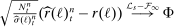 , where Φ is a standard normal random variable as in Theorem
 4.4 Some Extended Discussions
Here, we comment on the efficiency issue and on the behavior of our procedure under the rounding model of discrete prices.
4.4.1 Variance Reduction
 sequences satisfying the regularity conditions. We explain the procedure for
  defined in (21). Rewrite
  as
as  to indicate its dependence on
  . Let
. Let 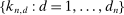 be a sequence of tuning parameters, and define the combined estimator
 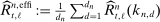 . As we know from other contexts (see, e.g., Abadie and Imbens (2006)), that averaging reduces variance, we just sketch the argument here. It suffices to consider the noise part:11

 is large. To see this, consider the sum
  , where

 has asymptotically negligible covariances if
  are sparse enough, for example,
  . As a consequence, the asymptotic variance of
  . The asymptotic distribution is entirely determined by
 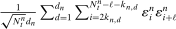 , that is, the three additional terms that appear in (11) from differencing will not affect the limiting variance. Therefore,
  (recall (22)) will be reduced since the asymptotic variance of the stationary noise becomes
  .
.4.4.2 Rounding Errors
The additive noise model (1) is the main framework in the literature, but there is a small but growing literature on rounding models that captures the effect of price discreteness; see, for example, Delattre and Jacod (1997), Rosenbaum (2009), and Li and Mykland (2015). Rounding of a continuous-state efficient price process can induce negative firs- order autocovariance in the observed returns similar to that induced by bid-ask bounce and infrequent trading (Schwartz and Whitcomb (1977)), and this effect may be particularly large when the nominal stock price level is low and when trading is frequent. Some applied papers in market microstructure have explicitly allowed for rounding errors, see, for example, Glosten and Harris (1988). Theoretically, the rounding model is difficult to work with in the very general semimartingale setting we have for the efficient price, and we have not so far managed to include this feature in our theoretical analysis. However, we do have simulation evidence suggesting that the ReMeDI estimator also works quite well in this case; see Section E.2 in Li and Linton (2022). Li and Mykland (2015) found that subsampling helps mitigate rounding errors. The ReMeDI approach shares something with subsampling methods in that it takes differences over long intervals. Perhaps this explains the superior performance of the ReMeDI estimators in the presence of rounding errors in the simulation experiments.
5 Simulation Study
5.1 Model Settings
 (24)
(24) ;
;  ;
;  ;
;  ;
;  ;
;  ;
;  ;
;  . This setting is motivated by some empirical facts that jumps in price levels and volatility tend to occur together; see Todorov and Tauchen (2011).
We further suppose that the stationary component of the microstructure noise follows an AR(1) process with Gaussian innovations  ,
,  ,
,  . Note that χ has unit variance. We set
  , motivated by the empirical studies in Aït-Sahalia, Mykland, and Zhang (2011) and Li, Laeven, and Vellekoop (2020).
5.2 LA versus ReMeDI
We estimate the autocovariances of microstructure noise using the ReMeDI estimator and the local averaging (LA) estimators (Jacod, Li, and Zheng (2017)). We assume that the noise is stationary so that we can compare the estimates to the true parameters. We also assume that the observation scheme is regular so that we know explicitly the data frequency, which is a key factor that affects the finite sample performance of many high-frequency estimators.
The top and middle panels of Figure 2 present the estimation of the first 20 autocovariances of the noise by ReMeDI and LA.12 The solid lines are the mean estimates over 1000 replications; the shaded region represents the 95% simulated confidence intervals. We simulate 23,400 observations for each sample path, corresponding to the number of seconds in a business day (6.5 trading hours). The ReMeDI estimators perform well: the estimates are approximately unbiased with narrow confidence bands. Surprisingly, there is a significant average deviation of the LA estimates from the true parameters, and the confidence bands are much larger as well.

Estimation of the autocovariances of noise by the ReMeDI method (top panel), the local averaging method (middle panel), and the bias-corrected local averaging method (bottom panel). The blue solid lines are the mean estimates of 1000 simulations by the three estimators. The tuning parameters of the ReMeDI and LA estimators are 10 and 6, respectively. The noise scale is fixed at γ ≡ 5 × 10⁻⁴.
The deviation of the LA estimates is elicited by a finite sample bias, which is known to be a fraction of the prior unknown quadratic variation (QV) of the efficient price; see the discussion in Jacod, Li, and Zheng (2017). Thus, to correct the bias, we need an estimate of the QV. But the estimation of QV in the presence of dependent noise is not trivial; see a discussion in Li, Laeven, and Vellekoop (2020). In a simulation context, we can obtain the QV and thus can give the LA estimators the privilege to make the bias correction, which is, of course, not feasible in practice. The bottom panel of Figure 2 displays the bias-corrected estimation of LA. Even with accurate bias correction, however, the ReMeDI estimators still outperform the LA estimators with almost no bias but greater accuracy.
It is interesting to compare ReMeDI and LA when the data frequencies vary. However, increasing the data frequency in a fixed time span has two effects: both the number of observations and the noise-to-signal ratio of tick returns will increase. We design a simulation study to separate the two effects and examine how sensitive ReMeDI and LA are to these changes.
The left panel of Figure 3 presents the mean squared error (MSE) of the ReMeDI and LA estimators for the first 20 autocovariances of noise. The sample size varies from 23,400 (1 trading day) to 117,000 (1 trading week), and 468,000 (1 trading month). The MSE of the ReMeDI estimators remains low and slightly drops when the sample sizes increases. The LA estimators, however, have larger MSE in a larger sample! This is statistically counterintuitive. However, it does make sense if we recall that the integrated volatility contributes to the finite sample bias of the LA estimators. Hence, a longer time span induces larger integrated volatility (relative to the number of observations), which in turn leads to a larger finite sample bias. This is especially so if the sample covers a period of volatility burst, and the likelihood of such an event increases if the sampling period becomes large; see our empirical studies with real transaction prices.

Mean squared error (MSE) of the ReMeDI and LA estimators for the first 20 autocovariances of noise based on 1000 simulations. In the left panel, the noise scale is fixed at γ = 5 × 10⁻⁴ and the sample size varies; in the right panel, the size sample is 23,400 while the noise scale parameter varies. The tuning parameters of the ReMeDI and LA estimators are 10 and 6, respectively.
The right panel of Figure 3 compares ReMeDI and LA when noise variance varies from 10−8 (small noise) to 10−6 (large noise). We note that the advantage of ReMeDI over LA is more prominent when the scale of noise is smaller. Indeed, the size of noise in practice is closer to the small noise scenario; see an extensive empirical study by Christensen, Oomen, and Podolskij (2014). Thus, in an extreme case when the noise has identical statistical properties in two samples, LA may give very different estimates due to the differences in sample sizes or noise-to-signal ratios. The ReMeDI approach remains robust and accurate.
5.3 Random Noise Size and Observation Times
As the last robustness check, we now allow for stochastic observation times and random scales of noise. Following Jacod, Li, and Zheng (2017), we let  follow an inhomogeneous Poisson process with rate
  , where
 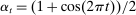 and the process γ satisfies
  ,
,  . We set
  ,
,  ,
,  ,
,  . Figure 4 reports the estimation of the autocorrelation functions by the two estimators. We observe similar patterns presented in Figure 2: compared to the ReMeDI estimators, the LA estimators have large biases with a wide confidence band.

Estimation of the autocorrelations of noise by the ReMeDI method (left panel) and the local averaging method (right panel). The blue solid lines are the mean estimates of 1000 simulations by the two estimators. The tuning parameters of the ReMeDI and LA estimators are 10 and 6, respectively. The noise has stochastic scales and the observation times are random; see the specifications in Section 5.3.
The Supplemental Material (Li and Linton (2022)) provides additional simulation studies to examine the quality of the CLT approximation, the effect of rounding error due to the discreteness of price, and the sensitivity to the choice of tuning parameters.
6 Empirical Study
We obtain the transaction prices of Coca-Cola (trading symbol KO)13 from the TAQ database for January 2018 (21 trading days). We remove prices before 9:30 and after 16:00. We collect approximately 50,000 observations per day, that is, 2.1 transactions per second on average. The average price is $46.84, with a standard deviation of 0.85.
Figure 5 plots the estimated autocovariances of noise by the ReMeDI estimators (the blue plots) based on samples of different sizes. The autocorrelation pattern is nontrivial: noise exhibits positive autocorrelations up to 4 lags, and shortly thereafter the sign switches to negative for a few lags, and then reverts to positive autocorrelations before decaying to zero around 20 lags. The pointwise confidence interval14 includes zero or excludes positive values after lag 5, which is incompatible with simple long memory.

Estimation of autocovariances of noise for Coca-Cola (KO) in January 2018. In the top panel, we use the transaction prices of KO on 2 January 2018; in the middle panel, we use the transaction prices of KO in the second trading week (8 January 2018 to 12 January 2018); we employ the entire transaction prices of KO in January 2018 in the bottom panel. The tuning parameters for ReMeDI and LA are 10 and 6, respectively. The shaded area in the top panel represents the 95% confidence interval, and we set in = 5,  to compute the asymptotic variances of the ReMeDI estimators, where
  is the number of observations.
The ReMeDI estimates of microstructure noise presented in Figure 5 are economically intuitive. The positive autocovariances at the first several lags may be a consequence of the order splitting strategies by high-frequency traders (Biais, Hillion, and Spatt (1995)), or the successive transactions executed by limit orders (Parlour (1998)).15 The negative autocovariances at the intermediate lags are consistent with the prediction of inventory models (Ho and Stoll (1981), Hendershott and Menkveld (2014)), in which the market makers induce negatively autocorrelated order flows to balance their inventories. However, the LA method gives very different estimates: it says that the noise is strongly autocorrelated without any sign of decay after 20 lags. This is economically counterintuitive—such a pattern, if it exists, would be exploited by high-frequency traders and we would expect it to disappear rapidly. Moreover, the serial dependence, according to the LA estimates, is even stronger when estimation is performed on a larger sample. Since we only estimate autocovariances of noise up to 20 ticks/lags, or a few seconds, it is statistically counterintuitive to obtain stronger autocovariance estimates using the prices of a week than using the prices in a single trading day. This is in line with our simulation study that the LA estimates are subject to a finite sample bias that depends on the noise-to-signal ratio and sample size. The ReMeDI approach retains its accuracy and robustness.
7 Concluding Remarks
We introduce a differencing method to separate the microstructure noise from the underlying semimartingale efficient price in a general setting. We demonstrate the robustness of the proposed method compared to the main existing approach. We have concentrated on the infill setting primarily and the univariate case. The method naturally extends to the multivariate case, although in that case, several issues arise. First, the nonsynchronous trading issue has to be faced. Second, even when the assets trade on a common clock, there are some remaining theoretical results that need to be established for the infill case. We discussed briefly in Section 4.4.1 how one can improve efficiency by combining the estimators associated with different choices of  . An alternative potential source of efficiency gain is from the heteroscedasticity delivered by the γ process, which was not exploited by our method. Given a consistent estimator of
  , one may implement a kind of feasible GLS procedure. We leave these problems for future research.
 , the mixing coefficients for k are given by

 ,
,  . The sequence
  is ρ-mixing if
  as
as  .
.
 if
if  and
and  if j is a singleton.
 in practice.
 leads to smaller bias.
 .
.
Appendix A: The Asymptotic (Co)Variance
 that appears in the asymptotic variance in Theorem 2. In the sequel, whenever we have two vectors
  ,
,  , we suppose without loss of generality that
  . We denote

 , there is an associated (unique) pair of subsets:
 (25)
(25) the following moments:16

 is given by
 (26)
(26)Appendix B: The Estimation of the Asymptotic (Co)Variance


 (27)
(27)
 (28)
(28)Now we consider some special cases where the asymptotic (co)variances are simpler. As a consequence, the asymptotic variance estimators are also much simplified.
 . The observations schemes that satisfy this condition include the regular sampling scheme and the time-changed regular sampling scheme. Next, let
  . One can verify that the modulated Poisson sampling scheme satisfies this condition; see the discussion in Jacod, Li, and Zheng (2017). The asymptotic (co)variance becomes