A General Framework for Robust Contracting Models
Abstract
We study a class of models of moral hazard in which a principal contracts with a counterparty, which may have its own internal organizational structure. The principal has non-Bayesian uncertainty as to what actions might be taken in response to the contract, and wishes to maximize her worst-case payoff. We identify conditions on the counterparty's possible responses to any given contract that imply that a linear contract solves this maxmin problem. In conjunction with a Richness property motivated by much previous literature, we identify a Responsiveness property that is sufficient—and, in an appropriate sense, also necessary—to ensure that linear contracts are optimal. We illustrate by contrasting several possible models of contracting in hierarchies. The analysis demonstrates how one can distill key features of contracting models that allow their findings to be carried beyond the bilateral setting.
1 Introduction
Suppose that a principal wishes to write an incentive contract to induce productive effort. How should she structure the incentives so as to optimally ensure their effectiveness? A rich theoretical literature has explored this question, giving arguments in favor of one or another form of contract.
However, this literature has generally focused on models involving a single principal and a single agent. In reality, agency often takes place beyond simple bilateral relationships. For example, the principal may be a firm or government office, procuring a good of unpredictable quality from a supplier, and committing to a payment that depends on the realized quality; but the supplier has its own internal agency problem, since the representative who signs the contract with the principal may not be the same worker who produces the good. Can we abstract away from the specificity of bilateral contracting models to understand when and why their lessons carry over to models of more complex organizations?
In this paper, we focus on one such lesson that has arisen frequently: that linear contracts—which simply pay some fixed fraction of the output produced—perform well by aligning the expected payoffs of the two parties. The literature on this theme has generally drawn on the idea that there may be a large space of possible actions by the agent, a notion that we formalize subsequently under the name of “Richness.” With a narrow space of possible actions, the structure of the optimal contract may be nonlinear and finely tuned to the known possibilities; but under richness, any such nonlinearities are vulnerable to strategic gaming by the agent. Incarnations of this idea have appeared in static moral hazard models (Diamond (1998), Carroll (2015), Barron, Georgiadis, and Swinkels (2020), Antić (2021)), dynamic moral hazard (Holmström and Milgrom (1987)), and screening as well (Malenko and Tsoy (2020)).
We focus more specifically on the following version of the argument, based on robustness to uncertainty: Consider a principal (“she”) and an agent (“he”), both risk-neutral, who agree to a contract that pays the agent 1/4 of whatever output he produces. Suppose that the principal does not know exactly what productive actions the agent is able to take, but she knows he has some action available that will give him an expected payoff of at least 1500 under this contract. Then, even without any information about what other actions are available, the principal can be sure the agent will get a payoff at least 1500 and, therefore, she gets at least 4500 for herself (since she receives 3/4 of output against the agent's 1/4). This argument was developed previously by Carroll (2015), which formalized this idea of a guarantee for the principal via a worst-case criterion, and showed more generally that linear contracts are optimal under such a criterion.
To see the difficulty in generalizing this conclusion beyond the simple bilateral setting, consider now a three-player hierarchy: The principal contracts with a supervisor (also “she”); the supervisor then subcontracts with an agent, and the agent chooses the action that determines output. Payments in both contracts are functions of output only. There are (at least) three natural ways to write this model, with different informational assumptions:
- (i) As in the bilateral model, the principal knows some actions available to the agent, but there may be other actions that she does not know about. The supervisor, however, fully knows the agent's production technology.
- (ii) The supervisor may know more actions than the principal does, but she suspects that the agent has still more actions available. Thus, the supervisor maximizes a worst-case objective with respect to unknown actions the agent may have; the principal has uncertainty over both the agent's possible actions and the supervisor's knowledge.
- (iii) The supervisor knows no more than the principal does; both of them face the same uncertainty about the agent's technology (and both maximize for the worst case).
We outline these three models more carefully in Section 2. All three of them allow a large space of possible actions by the agent, and indeed, all three satisfy our formal Richness condition. Yet, it turns out that linear contracts maximize the principal's worst-case criterion in models (i) and (ii), but not in model (iii) in general. (This will be shown in our later analysis.) Thus, the details of the model matter, and it may not be initially obvious what, beyond Richness, is needed.
Our paper aims to identify the additional condition at a high level of generality—and, in the process, obtain a better understanding of the essential ingredients behind the linearity argument. To do this, we abstract away from any particular organizational form. Instead, the principal contracts with a counterparty of unspecified structure. The principal's uncertainty about the environment is described by a correspondence Φ, where  specifies the distributions over output that she thinks may potentially arise when she offers contract w. The principal wants to choose w to maximize her expected net profit in the worst case. Throughout, we maintain the background assumptions that the principal is risk-neutral and uses the worst-case criterion; the focus is on understanding the properties of Φ that are central to the linearity argument.
We formalize the Richness property by requiring that, whenever some distribution over output is a possible response to a given contract w (i.e., lies in  ), any other distribution with the same expected output but higher expected payment to the counterparty is also possible. That is, the counterparty has the flexibility to extract maximal payment for a given expected output. In this form, it is clear that Richness by itself cannot pick out linear contracts, since it says nothing about how Φ varies when the contract changes.
The needed additional property that we identify is Responsiveness, which expresses that the counterparty's behavior responds to the incentives provided by expected payment. Responsiveness requires that when one contract w is replaced by a new contract  , such that every distribution that might have been chosen in response to w earns a higher expected payment than before, while some other distribution not chosen under w earns a lower payment than before, this unchosen distribution remains unchosen.
We show that the Richness and Responsiveness properties together imply that linear contracts give the best guarantees for the principal.1 This allows the lesson about the robustness of linear contracts to apply to a broad class of models of contracting with diverse organizational forms. We formally develop the general framework, define Richness and Responsiveness, and present this result in Section 3.
Having noted that, as a supplement to the Richness property, Responsiveness is sufficient to make linear contracts optimal, we next ask if it is also necessary. To address this question, in Section 4, we give a converse result. For this, we develop an auxiliary framework in which contracts specify payment as a function of a physical outcome, and Φ describes the counterparty's behavior in response to such contracts; the principal's value for each possible outcome is a separate parameter of the model. (For example, one can think of a supplier that can produce different goods, and a contract specifies a payment for each. How the supplier reacts to any given contract is independent of how much the principal values each good.) The Responsiveness property and a strengthened version of Richness can be expressed in this setting. When they hold, our main linearity result immediately implies that the principal can always maximize her guarantee by offering a linear contract, meaning one that pays proportionally to the principal's value for the realized outcome. Our converse shows that, once we ignore certain contracts that can be ruled out a priori as never optimal, if Responsiveness is violated, then there exists a valuation for the principal under which linear contracts are not optimal. This shows that our Responsiveness condition captures, at a formal level, the specific cross-contract restriction on behavior needed for the linearity result.
After presenting the results above, in Section 5 we analyze the robust principal-agent model and hierarchical models (i)–(ii) sketched above in more detail to indicate how the Richness and Responsiveness properties can be verified. (The Online Supplementary Material, Walton and Carroll (2022), in Section S-1, presents two further applications to illustrate the breadth of our framework.) Section 6 examines hierarchical model (iii), where Responsiveness is violated and linear contracts can fail to be optimal.
A reader might think that our whole exercise is unnecessary because the models where linear contracts turn out to be optimal can be easily reduced to bilateral contracting models anyway. This reaction is misplaced. For example, one might try to reduce hierarchical model (i) to a robust principal-agent model by combining the supervisor and agent into a single entity, whose cost of producing any output distribution is defined as the cost for the supervisor to induce the agent to choose that distribution in the original hierarchical model. However, this reduction fails because it does not preserve the structure of uncertainty needed to apply the result from the robust principal-agent model. In Section 7, we explain this failure in further detail. We also describe what the worst-case environment in the hierarchical model actually looks like; it is quite different from the worst-case in the principal-agent model.
Although the substantive results in this paper concern linear contracts, our conceptual framework more generally offers a way to express and prove results for contracting models without relying on a particular organizational structure. Robustness arguments for linear contracts naturally call for such a framework, because, as Section 7 shows, there does not seem to be any easy reduction argument that would allow us to directly extend the results from bilateral environments to more complex ones. In principle, the same methodology is applicable in the analysis of other forms of contracts and properties of contracting models that favor them. To illustrate by example, we demonstrate, in Section S-3 of the Online Supplementary Material, a result on concave contracts analogous to our main theorem on linear contracts: under Responsiveness and a particular weakening of Richness, concave contracts are optimal.
Our work connects to several branches of literature. First, it naturally relates to the body of work on linear contracts and their robustness against large spaces of actions, mentioned previously. While many of the arguments in this literature are thematically related, which helps motivate our interest in focusing on linear contracts, we certainly do not claim that all of these previous findings are special cases of the results developed here. Also related is the literature explaining other kinds of simple incentive structures as robust in unknown environments, such as Frankel (2014), Garrett (2014), and Carroll and Meng (2016).
There is also considerable previous work on incentives in hierarchies and more complex structures, mostly focusing on comparison across organizational forms (surveyed in Mookherjee (2006, 2013)). (There is a separate and more distant strand of literature on hierarchies, such as Tirole (1986), that focuses on issues of collusion.) Yet there seems to be little work studying how organizational structure interacts with the optimal choice of contractual form.
Finally, closest in spirit to the present work are several recent papers that study robust moral hazard contracting in different organizational environments. In particular, there is the work of Dai and Toikka (2022), which studies robust incentives for a team (and which inspired one of the additional applications explored in the Online Supplementary Material). Others in this line are Marku, Ocampo, and Tondji (2022), which takes up a common agency model, and Kambhampati (2022), which considers two agents who produce independently but are known to share a common technology.
2 Overview of Examples
We begin with brief descriptions of our main example applications, meant to give context for the general framework introduced in Section 3. The examples will be presented in formal detail in Section 5.
Robust Principal-Agent Model. In the basic application, the principal contracts directly with an agent, offering a contract that specifies payment as a function of output. Limited liability applies (in this example and throughout the paper): the contract can never pay less than zero. The agent can take any of various actions; an action is modeled as a pair, consisting of a probability distribution over output and a (nonnegative) effort cost incurred by the agent. The principal knows of some set of actions that are definitely available to the agent. But the principal does not know the true production technology, that is, the set of actions actually available. For any contract she can offer, she evaluates it based on her guaranteed payoff, that is, her expected net profit (after paying the agent) in the worst case over all possible technologies consistent with her knowledge. The guarantee of a contract is typically strictly positive, because the principal knows that the agent is optimizing under the true production technology, so will not take a totally unproductive action if he is known to have a better action available. The analysis of Carroll (2015) showed that the best guarantee for the principal is attained by a linear contract, and we shall recover this result as one instance of our general framework.
Hierarchical Model (i). In this model, the principal offers a contract to a supervisor, again specifying (nonnegative) payment as a function of output. The supervisor, after seeing this contract, in turn offers a contract to the agent, also specifying (nonnegative) payment as a function of output. The agent privately chooses his action, output is produced, and then both the supervisor and agent are paid according to their respective contracts.
In this model, we assume that the supervisor knows the agent's technology, so when she writes a contract, she is solving a standard, Bayesian version of a principal-agent problem, in which the “output” produced by the agent is not the output in the original model but rather the payment received by the supervisor. The principal, as before, knows only some actions available to the agent, but does not know the full technology, and evaluates contracts by the worst-case expected payoff over possible technologies.
Hierarchical Model (ii). The hierarchical structure is as in the previous model, but now the supervisor's knowledge is different: she may know of actions that the principal does not, but is uncertain as to whether there are still more actions available, and writes her contract with the agent to maximize her own worst-case guarantee. Note that the relationship between the supervisor and the agent is now described by the robust principal-agent model above; this implies that the supervisor has an optimal contract in which she offers the agent some fixed fraction of the payment she receives from the principal.
The principal does not know the full technology, nor how much of it is known by the supervisor, and again uses the worst-case criterion.
Hierarchical model (iii). In this version of the hierarchical model, the supervisor and the principal are symmetrically uninformed: the supervisor knows only as much about the technology as the principal does, and (as in model (ii)) maximizes a worst-case guarantee when contracting with the agent.
Model (iii) can be expressed in the language of our general framework below, but it does not satisfy the conditions for our linearity result (in particular, the Responsiveness property is violated), and indeed the result may fail, as we shall show in Section 6.
In Section S-1 of the Online Supplementary Material, we give two more examples to illustrate the breadth of potential applications for our framework. In the first example, a supervisor contracts with a team of two agents who play differentiated roles in producing output. The second example is a simplified version of the model of Dai and Toikka (2022); the principal contracts directly with a team of agents, and we simply assume that payments to the team are split equally among the agents.
One might argue that these models make some demanding assumptions. The limited liability restriction, which we maintain throughout, may be less natural in the kinds of firm-to-firm settings where hierarchies naturally arise than it would be in contracting with individuals.2 In addition, hierarchical models (ii) and (iii) impose the worst-case criterion as a positive description of the supervisor's behavior, unlike in the principal-agent model, where worst-case maximization can be viewed simply as a language for expressing statements about robustness properties of contracts. Nonetheless, our goal here is not to write down the most defensible model of contracting in hierarchies, but simply to illustrate that there are various models one could consider, only some of which deliver linear contracts, and thereby to motivate the search for their common features.
3 Main Framework and Result
First, some notational conventions. We write  for the space of Borel distributions on a metric space X. We equip
  with the weak topology. For
  ,
,  is the degenerate distribution putting probability 1 on x. We also write
  for the set of nonnegative real numbers, and equip it with the usual topology. We write
  for the convex hull of X, when
  . We write
  for the space of continuous functions from X to
  , equipped with the sup-norm,
  . Recall that when X is compact,
  is a Banach space. We write
  for the subset of
  consisting of functions whose values lie in
  .
.
3.1 The Modeling Framework
There is a principal, who contracts with a counterparty, which will subsequently produce (stochastic) output that accrues naturally to the principal. The principal can provide incentives by promising payments to the counterparty.
There is an exogenously given set  of possible output values. We assume Y is nonempty and compact, and normalize
  , and denote
  . A contract is a function
  .3 Note that this definition incorporates the limited liability restriction: the contract must pay a nonnegative amount.

 is a constant. The special case
  is called the zero contract.
We take as given a nonempty-valued correspondence  , the outcome correspondence.
  describes the set of distributions over output y that the counterparty may generate in response to contract w, from the principal's point of view. The multiple-valuedness of
  thus reflects the principal's uncertainty (about the production technology, or other aspects of the environment). Note that the interpretation of
  is not simply that distribution F may be physically feasible, but rather that it might actually occur in response to contract w. For example, if the principal knows that the counterparty is able to produce output 0 with probability 1, but would never do so in response to w because some other distribution is better incentivized, then we would have
  . For now, we treat the correspondence Φ as exogenously given; in each of the individual applications in Section 5, we will in turn define Φ from more primitive objects.

We now consider the following properties that Φ may have.
Richness.Suppose  ,
,  , and
, and  is another distribution such that
  and
and  . Then
  .
.
This property essentially says that the set of possible responses to a given contract is sufficiently broad: for any distribution that the counterparty might produce, any other distribution with the same expected output but higher average payment to the counterparty is also possible. Even more simply put, for any given expected output, the principal worries that the counterparty will extract the highest possible average payment.
Responsiveness.Suppose  and
and  such that
  . Suppose that
  for all
  , while
  . Then
  .
.
This property expresses how the possible outcomes respond to the incentives provided by expected payment. If an “old” contract w is replaced by a “new” contract  , such that any distribution that the counterparty might have produced under the old contract now pays more (in expectation) than before, while some other distribution F pays less than before, the counterparty will not switch to choosing F.
One way to understand Responsiveness is to consider a standard principal-agent problem without uncertainty: The counterparty is a single agent, and there is some fixed, mutually known set of output distributions F that he can produce, each with an associated cost  . When the principal offers contract w, the agent chooses F to maximize
  . Thus
  is the set of maximizers F. This model satisfies Responsiveness: Consider any
  , and
, and  for which the hypotheses of Responsiveness are satisfied. If F is not even feasible, clearly
  . Otherwise, F is feasible but not optimal under w. Then let
  be an optimal choice. So
  . Since
  while
while  , we have
  , that is, F remains nonoptimal under
  .
.
Intuitively, we would expect Responsiveness to be satisfied when the counterparty is a single agent who maximizes expected value as in the example above, or more generally, when the counterparty has a “leader” who understands the environment and maximizes expected value (such as the supervisor in hierarchical model (i)). But it also turns out to be satisfied in some other models, such as hierarchy (ii) where the leader is not expected-value-maximizing. We discuss further in Section 5.3.
For simplicity, we have not included a participation constraint. An earlier version of the paper (Walton and Carroll (2019)) describes how such a constraint can be accommodated, by restricting the principal's choice of contracts to a subset of  , interpreted as the set of contracts that the counterparty is sure to accept, and assuming an appropriate structure on this subset.
3.2 Linearity Result
Now we come to the first main result: our conditions are sufficient for optimality of linear contracts.
Theorem 1.Suppose the correspondence  has the Richness and Responsiveness properties. Then, for any contract w, there is a linear contract
  such that
  .
.
We prove Theorem 1 constructively, by using the worst-case scenario under w to determine the slope of  . The argument is illustrated in Figure 1. First, for any given level of expected output, say μ, Richness ensures that the principal is worried about the highest expected payment ν; this highest expected payment is given by the concavification of w, call it ŵ. Concavity of ŵ implies that the ratio
  , the expected payment per dollar of expected output, is decreasing in μ. So, among all distributions in
  , the one with the lowest expected output μ is also the one for which the fraction of output ceded to the agent is highest; hence, this must be the worst-case distribution. The resulting outcome is shown as point
  in Figure 1. We then take
  to be the linear contract that passes through this same point. Under
  , the payment-per-output ratio is constant, so this new contract both pays more than the old one for higher expected output and pays less for lower expected output. By Responsiveness,
  can only motivate the counterparty to produce higher expected output than w—which in turn means higher expected profit for the principal, since linearity ensures that expected output and expected profit are aligned.

Constructing a linear contract w′ with as good or better guarantee than some initial contract w.
The above proof sketch is imprecise about the distinction between weak and strict inequalities, and also implicitly assumes that the inf in the definition of  is attained, which it may not be. The full proof below fills in these gaps. While we have used the concavification ŵ for intuition, the formal proof does not need to refer to it.
Proof.We may assume that  , since otherwise we can just take
  to be the zero contract. Now, let
  . Note that this expression is well-defined, since every
  satisfies
  . In fact, for every
  , we have
  , and thus λ is bounded above by
  .
.
Now define the linear contract  . We will show that
  .
.
Let  be a sequence of distributions in
  approaching the inf in the definition of
  :
:  . By taking a subsequence, we can assume that
  converges to some limiting distribution
  . Put
. Put  ,
,  and
and  . Since
  for each k, we have
  . We claim that equality must hold. If not, pick
  with
with  . By definition of λ, there exists
  such that
  . Since
  , we have

 as well. Take
  to be an appropriate convex combination of
  and
and  so that
  . Then we have
  (since the latter inequality holds both for the component
  and, trivially, for
  ). Hence, either
  , or else we can apply Richness to the distributions
  and
and  to conclude
  . Either way,
  contains a distribution with expected output
  and expected payment at least
  . This means that
  . But taking
  gives
gives  , a contradiction. Thus, we conclude
  as claimed.
This implies that  . We can complete the proof by showing that
  . Since every distribution F satisfies
  , it suffices to show that
  for every
  .
.
Consider any distribution  such that
  ; we need to show
  . Put
. Put  . Let F be a convex combination of
  and
and  such that
  . We have
  , since this inequality holds both for the component
  and (trivially) for
  . Since
  , we have
  . Moreover,
  , while for every
  , we have
  ; thus, Responsiveness implies
  . Since F has the same expected output and the same expected payment under
  as
as  does, Richness then implies
  . Q.E.D.
This shows that Richness and Responsiveness are sufficient for linear contracts; but are they necessary? In Section 4, we will give a converse result that aims toward addressing this question.
For the moment, we simply note that neither property can be dropped entirely. Richness alone would not give us the result, since we clearly need some assumption on how  varies with w. For a more concrete example, in Section 6 we will note that in hierarchical model (iii), Φ satisfies Richness, but the conclusion of Theorem 1 can fail.
To see that Responsiveness alone is not sufficient, just consider a standard principal-agent problem without uncertainty, as was used to illustrate Responsiveness above. As is well known, usually a nonlinear contract is strictly optimal. For example, under standard specifications with a discrete output space and just two possible distributions F, an optimal contract pays only for the one realization of output that achieves the highest likelihood ratio, and pays zero for all other realizations.4
3.3 Existence of Optimum
We have still been imprecise on one point: The verbal interpretation given to Theorem 1 is that a linear contract is optimal for the principal. Indeed, if an optimal contract exists, then there is one that is linear. However, it may happen that no optimal contract exists. In this case, under the conditions of Theorem 1, the supremum payoff  is approached, but not attained, by linear contracts.
It can be useful to have a handy way to check that existence is indeed satisfied in any given model. Define the correspondence  by
by  (recall that
  was the linear contract of slope α).
Proposition 2.Suppose that Φ satisfies Richness and Responsiveness. If moreover  is lower hemicontinuous, then there exists a contract maximizing
  (and, in fact, the maximum is attained by a linear contract).
The proof (a straightforward limiting argument) is in the Appendix. In the examples in Section 5, we use this result to show that an optimal contract exists.
4 A Converse Result
We have argued that, given Richness, the addition of Responsiveness is sufficient for optimal contracts to be linear. To argue that we have really identified the right condition, we should show that Responsiveness is necessary as well. Of course, in the framework so far, this cannot be exactly right: many contracts are clearly far from optimal (e.g., any contract that always pays more than the value of output), so violations of Responsiveness among such contracts are irrelevant. This suggests we should look for a more general framework, in which Responsiveness can be defined at the level of a class of models, so that Responsiveness becomes necessary to ensure that all instances within the class deliver linear contracts.
Specifically, we will now consider a framework in which output is not directly measured in payoff units. Instead, the counterparty produces “physical” outputs, for example, the counterparty may be a supplier that can produce different types of goods. Contracts specify payment as a function of the physical output. The principal, in turn, derives some monetary value from each possible physical output. The principal's valuation of outputs is now an additional parameter in the model; it matters for the principal's preferences but is irrelevant to the counterparty's behavior. Here, Responsiveness will be sufficient to ensure that, no matter what this valuation is, a linear contract (one that pays proportionally to the principal's value) is optimal, and we will argue that Responsiveness is essentially necessary for this conclusion as well.
Thus, for this section only, we consider a given nonempty set Z of physical outputs. We take Z to be finite (and endowed with the discrete metric), and we denote a typical element by z. A contract is now a function  . We take as given a nonempty-valued outcome correspondence
  .
.
We reformulate the Richness property for this setting as follows:
Strong Richness.
- (a) Suppose
 ,
,  , and
, and  such that
  . Then
  .
. - (b) For every
 , the set
  is closed.
Part (a) of this property is stronger than our original Richness property because it drops the restriction that F and  should have the same expected output; this restriction cannot be formulated when output does not have a numeric value. We do not view this loss as a major sacrifice. In our applications in Section 5, this restriction matters only because it allows us to include tie-breaking assumptions on the counterparty's behavior (e.g., assuming that if the agent is indifferent between multiple distributions, he chooses the one that is better for the principal); without such assumptions, an optimal contract can sometimes fail to exist. Part (b) of Strong Richness is a technical condition that helps rule out some inconvenient boundary cases.
Together, parts (a) and (b) imply that, for each w, there exists a threshold  such that
  .
.
We can formulate Responsiveness exactly as in our main framework, since it made no reference to the value of output.
Responsiveness.Suppose  , and
, and  such that
  . Suppose that
  for all
  , while
  . Then
  .
.
 such that
  . For any valuation and any contract, the principal's guarantee is then defined as

 in our previous framework.
We can now say that a contract w is linear given v if there exists a constant  such that
  for all z.
We will also say that w is grounded if  . We will focus our attention on grounded contracts (note that, given any v, any linear contract is grounded). This is justified if, for example,
  whenever w and
  are two contracts that differ by a constant: then, if a contract is not grounded, the principal can subtract a constant from it without changing incentives and so improve her own payoff. (All of our example applications satisfy this property of invariance to constant translations.)
Suppose that Φ satisfies Strong Richness and Responsiveness. Theorem 1 implies that, given any valuation v, for any contract w, there is a contract  that is linear given v and satisfies
  .
.
A conjecture might be that this conclusion fails whenever Responsiveness is violated: that is, if Φ satisfies Strong Richness but not Responsiveness, there exists some choice of valuation v for which a nonlinear contract gives a strictly higher guarantee than any linear one. We will show a slightly weaker version of this statement: Given Φ, some contracts can be quickly ruled out as never optimal regardless of v, except in degenerate cases. We can think of these contracts as “irrelevant.” We will show that if there is a violation of Responsiveness involving “relevant” (and grounded) contracts, then v can be chosen so that a nonlinear contract does better than linear.
Given Φ satisfying Strong Richness, let h be the threshold function defined above; and, for  and
and  , write βw for the contract obtained by scaling w pointwise by β.
Now say that a contract w is scaling-dominated if, for every v such that  , there exists some
  such that
  . These are the contracts we regard as irrelevant. They can be identified as nonoptimal using only a very small part of the correspondence Φ (namely, its values on the scalar multiples βw). Thus we can identify whether w is scaling-dominated using only the values of h on its scalar multiples, and the next proposition characterizes explicitly when this happens.
Proposition 3.Assume Strong Richness, and let w be a grounded contract. Then w is scaling-dominated if and only if it satisfies at least one of the following five conditions:
- (i)
 .
. - (ii) There exists
 such that
  .
. - (iii) For every positive number K, there exists
 such that
  .
. - (iv) For every number
 , there exists
  such that
  and
and  .
. - (v) There exist
 and
and  such that
  and
and

Moreover, if none of these conditions is satisfied, we can choose v such that w is linear given v,  , and
, and  for all
  .
.
With our focus on contracts that are not scaling-dominated, we can now give our statement on the necessity of Responsiveness.
Theorem 4.Assume Φ satisfies Strong Richness but fails to satisfy Responsiveness between some two contracts  , where
  is grounded and not scaling-dominated. Then the valuation v can be chosen so that w gives a strictly higher guarantee than any linear contract.
The proofs of Proposition 3 and Theorem 4 are left to the Appendix; we just give sketches here.
For the “if” direction of Proposition 3, we go through the conditions one by one. In each case, we use the statement of the condition to identify the relevant rescaling βw that does better than w. (In conditions (iii) and (iv), where β depends on K, we must first choose K appropriately depending on the valuation v.) For the “only if” direction, it suffices to prove the last statement of the proposition; thus we wish to choose v to be proportional to the given contract w (thus making w linear) and pick the constant of proportionality so that w is in fact optimal among linear contracts. Writing down the conditions needed for this to happen, it turns out that we run into difficulty precisely when one of (i)–(v) holds.
For Theorem 4, the key observation is that when Responsiveness is violated between contracts  , and
, and  is linear, then w gives a strictly better guarantee than
  does. (Refer back to Figure 1: a violation of Responsiveness means that some low-output distributions are possible under
  but not under w.) Thus, to prove Theorem 4, we can invoke the last statement of Proposition 3 to choose v such that the given
  is optimal among linear contracts. The foregoing observation then implies that w does strictly better than
  , and thus better than any linear contract.
As a final remark, we note that the lengthy conditions in Proposition 3 can be somewhat simplified if we assume that Φ satisfies the following additional property.
Scaling Monotonicity.For any  and any
  ,
,  .
.
Given Strong Richness, this property is equivalent to the statement that  is weakly increasing in β. In words, it says that the counterparty responds positively to rescaling of incentives (but does not say anything about responses to changes in the shape of incentives). It is satisfied in the robust principal-agent model and all three versions of the hierarchical model.
 , (iv)
  , (v)
, (v)  , where

5 Applications
We now return to our main framework where output  is directly measured in payoff units. We proceed to detail the various applications that were previewed in Section 2, showing how they are instances of the general framework. We indicate how to verify Richness and Responsiveness, as well as lower hemicontinuity. (Some of the formalities are deferred to the Online Supplementary Material.) Hierarchical model (iii) does not satisfy Responsiveness and so is left to the next section.
5.1 Robust Principal-Agent Model
 . If action
  is taken, output is drawn according to the distribution F and the agent incurs an effort cost of c. We define a technology to be a nonempty, compact subset of
  , interpreted as the set of actions available to the agent. Given a contract
  and technology
  , the agent maximizes objective

 . We assume that the principal does not know
  . Instead, there is an exogenously given technology
  , representing all actions that are known by the principal to be available to the agent. The agent's actual technology is known only to satisfy
  .
. ; this is the set of distributions that can result when the agent maximizes
  over
over  given w. Continuity of w and compactness of
  ensure that
  is nonempty. Finally, as a tie-breaking condition, we assume that when the agent is indifferent among actions, he chooses the one best for the principal; we call such actions principal-preferred. Formally, this set is denoted as
  . This assumption helps to ensure that an optimal contract w exists (discussed more momentarily). Now the outcome correspondence is defined as

 .
.This is the same model as the one considered in Carroll (2015). In our framework, we reproduce the main result of that paper, by verifying that Richness and Responsiveness hold in this model. We also verify that the restricted correspondence  is lower hemicontinuous, so a maximizing linear contract exists; this existence is needed later when we embed this model in a principal-supervisor-agent hierarchy, as it ensures that the supervisor's behavior is well-defined.
Proposition 5.There exists a linear contract maximizing  .
.
Essentially, Richness holds because, for any F that might be chosen for some technology, the more-remunerative  might then also be chosen if it turned out to also be available. Responsiveness holds by the same argument as in the principal-agent model without uncertainty sketched in Section 3.1, repeated for each possible technology. The formal proof ends up a bit lengthy because of tie-breaking technicalities.
Proof.(Richness) Let  ,
,  , so that there exists a technology
  containing action
  such that
  for all
  . Let
. Let  such that
  and
and  . Consider an alternative technology
  . Then

 , so
, so  . If
. If  , then F being principal-preferred implies that
  is principal-preferred in
  . Otherwise,
  , and hence the agent strictly prefers taking action
  to all other actions in
  , so
, so  is principal-preferred since it is the only element of
  . So
. So  .
.(Responsiveness) Let  and
and  satisfy the conditions of the Responsiveness property. If we can show for any technology
  that
that  , then
  . Take any technology
  containing
  for some
  , and take
  . By the hypothesis of Responsiveness and agent optimality,
 (1)
(1) . Otherwise, they are all equalities. In this case, it is possible for
  only if
  and
and  as well. If this holds, principal tie-breaking under w and the hypothesis of Responsiveness along with the equalities in (1) imply

 , so
, so  .
.Now we have verified Richness and Responsiveness, so by Theorem 1, we can restrict to linear contracts when maximizing  . It remains to verify that
  is lower hemicontinuous.
(Lower Hemicontinuity) Let  ,
,  , and let
  be an open neighborhood of F in
  . We want to show that there exists
  such that
  implies that
  is nonempty, where
  is the Euclidean ball of radius η around α restricted to
  .
.
If  , then any technology
  containing
  has
has  for any
  , and F is principal-preferred, giving
  already. So we can assume that
  . Then choose
  such that
  .
.
Let  be a technology for which the agent produces distribution F. We can assume without loss that
  . By Berge's theorem,
  defined by
  is continuous.
We claim that there exists some η such that  implies
  . If
. If  , then this claim follows from the fact that
  together with continuity of
  . So focus on
  , and suppose no such η exists. Then there is some sequence of
  and corresponding optimal actions
  , which we can assume (by taking a subsequence) converge to
  , where
  . This contradicts that F has largest mean among zero-cost actions in
  (which follows from principal-preferred tie-breaking).
Hence, for any  , constructing new technology
  yields
  as the unique maximizer of
  over
over  , so
, so 

 , and
, and  . Q.E.D.
One comment on interpretation: The above proof relies (as do many others later) on adding an arbitrary action of the form  to the technology. It may seem unrealistic to allow the agent to produce large amounts of output at zero cost. However, the fact that the unknown actions are totally unrestricted is not crucial; the logic can be carried over to more detailed models that incorporate lower bounds on plausible effort costs. (See Carroll (2015), Section II.A, for more details.)
5.2 Hierarchical Model (i)
The three hierarchical models that we analyze have the following structure. The principal contracts with a supervisor, who, after observing this contract, writes a contract with an agent. We assume that, for reasons outside the model, the principal cannot contract directly with the agent. We assume that the supervisor does not directly affect production in any way; the only role the supervisor plays is as an intermediary between the principal and the agent. Technology for the agent is the same as in Section 5.1. The contract from the principal to the supervisor is the w of our general framework; the contract from the supervisor to the agent is denoted  , and we assume both contracts depend solely on output, so that
  .
.
The agent's objective is the same as in the robust principal-agent model, but now the agent receives payment from the supervisor, not directly from the principal. Thus, given contract  and technology
  , the agent maximizes objective
  over
over  .
.
In all versions of the hierarchical model, we assume that the principal does not know  . Like the robust principal-agent model, there is an exogenously given technology
  , representing all actions known by the principal to be available to the agent. Let
  be defined as before, noting that
  refers to the contract between supervisor and agent (henceforth “S-A contract”).
In hierarchical model (i), we assume that the supervisor is perfectly informed of  , which must include the actions known to the principal, that is,
  . The supervisor wants to maximize the expected difference between payments from the principal and payments to the agent. In addition, we restrict the set of permitted S-A contracts to some exogenously given compact set
  , which is assumed to contain all linear contracts with slope in the interval
  . This assumption is necessary to ensure the supervisor always has a best reply. (Without some such restriction, one can find situations, similar to Mirrlees (1999), in which no optimal contract for the supervisor exists. See the earlier version, Walton and Carroll (2019), for an example and more discussion.)
 and
and  , define
 . Thus
  is the set of distributions that are best for the supervisor among the agent's optimal choices. This again represents a tie-breaking condition, and we refer to elements of
  as supervisor-preferred. The supervisor's objective in hierarchical model (i) is then

 is a slight abuse of notation: this is a set of distributions, not a single distribution, but the expectation is well-defined since it is the same for all distributions in this set (and the set is nonempty; see the proof of Lemma 6 below). The “i” in
  stands for “informed.”
 . Now define

 , this is the set of output distributions that are possible, given that the supervisor is choosing contract
  to optimize
  , and the agent is maximizing given
  , along with the tie-breaking conditions.
 .
.This completes the description of the model. We should make sure  is nonempty-valued; this is done in the lemma below.
Lemma 6.For each w,  is nonempty.
The proof of this lemma, and remaining proofs in this section, are deferred to the Online Supplementary Material, as they are either technical or similar to previous proofs.
To analyze the model, it helps to restate the definition of  . The distribution F lies in
  if and only if there exists a triple
  , where
  is a technology,
  , and
, and  , that satisfies the following conditions:
- (a) Supervisor maximization: the contract
 maximizes
  over
over  ;
; - (b) Agent maximization: action
 lies in
  and, given contract
  , this action maximizes the agent's payoff over
  ;
; - (c) Supervisor-preferred tie-breaking: given
 , action
  maximizes the supervisor's payoff over actions satisfying (b);
 - (d) Principal-preferred tie-breaking: given
 , action
  maximizes the principal's payoff over actions satisfying (b)–(c).
A triple  satisfying these conditions will be called a PSA(i)-certificate for F under w.
The following lemma shows that in searching for such a certificate, we can focus on cases where  and
and  (recall that
  denotes the zero contract).
Lemma 7.For any w and F, we have  if and only if there exists a PSA(i)-certificate for F under w of the form
  .
.
To see why this is, take the following perspective on the supervisor's problem: Any choice of contract  will induce the agent to produce some distribution F. Rather than view the supervisor as choosing
  , we can view her as directly choosing what F to induce, and then inducing it in the least costly way. Now, if there is some technology
  under which the supervisor would choose to induce F, then under
  , the supervisor is all the more inclined to induce F, since she can do so costlessly by offering the agent the zero contract. The lemma follows from this observation, together with careful verification of the tie-breaking conditions.
We can now show that the model falls under our general framework, and thus we have the following.
Proposition 8.There exists a linear contract maximizing  .
.
We verify the Richness and Responsiveness properties, as well as the lower hemicontinuity property, by arguments very similar to those used in the robust principal-agent model. Along the way, Lemma 7 helps to simplify by reducing the space of possibilities to consider.
5.3 Hierarchical Model (ii)
Hierarchical model (ii) closely resembles the previous hierarchical model. The key difference is that the supervisor is not perfectly informed of  . Instead, the supervisor is now uncertain about
  but we assume she is at least as well informed as the principal is. Specifically, the principal knows about technology
  , the supervisor knows about technology
  , and the true technology is
  , with
  . The principal, for her part, is uncertain about both
  and
and  . Since the model continues to focus on the principal's problem,
  is a primitive of the model, whereas
  and
and  are free variables. We also no longer restrict the supervisor to contracts in
  , since such a restriction will not be needed for existence of an optimal S-A contract; thus the supervisor may offer any contract
  .
.
 and
and  as in hierarchical model (i). The supervisor's objective in hierarchical model (ii) is

 is the informed supervisor objective of hierarchical model (i), and
  is the supervisor's knowledge of the technology. We write “u” to denote “uninformed.” In words, the supervisor maximizes expected money received minus money paid, given the agent's strategic response, in the worst case over all possible technologies containing
  .
. , define

 from hierarchical model (i). It now depends also on
  since this determines the supervisor's behavior.
 .
.As before, we should check nonemptiness.
Lemma 9.For each w,  is nonempty.
We comment that this is where we use the lower hemicontinuity result from the robust principal-agent model: it ensures that the supervisor has an optimal choice of  —in fact, one in which
  is proportional to w—so that the union in the definition of
  is not empty.
To analyze the model, we proceed in a fashion similar to the previous hierarchical model. Distribution F is in  if there exists a situation in which the agent would choose it—where now such a situation is described by a quadruple
  , meeting conditions analogous to (a)–(d) in hierarchical model (i). We refer to such a quadruple as a PSA(ii)-certificate for F under w. We can formulate an analogue of Lemma 7 for this model (see Lemma S-6 in the Online Supplementary Material): F lies in
  if and only if there exists such a PSA(ii)-certificate in which
  ,
,  and, moreover,
  .
.
This fact is useful in showing that the model satisfies our two properties, and thereby obtaining our linearity result.
Proposition 10.There exists a linear contract maximizing  .
.
Again, the proof follows the same basic argument as for the principal-agent model (and as for hierarchical model (i)).
It might not be obvious that this model satisfies Responsiveness, since the supervisor is no longer modeled as an expected-utility maximizer. However, the key is that Responsiveness is a property on the correspondence Φ, which gathers the counterparty's behavior across all possible environments (in this case, all possible  and
and  ); it does not have to hold in each environment individually. In this model, Lemma S-6 shows, in effect, that we can restrict attention to a crucial subset of possible environments: those in which the supervisor knows that she can induce distribution F for free by offering the zero contract, and she chooses to do so. In this subset of environments, the supervisor does act like an expected-utility maximizer, and this suffices to imply Responsiveness.
6 An Example Where Responsiveness Fails
In this section, we describe version (iii) of the hierarchical model, where the principal is no longer uncertain as to what the supervisor does and does not know. Instead, the supervisor, like the principal, knows only that the technology  is a superset of the given
  , and she contracts with the agent so as to maximize her own worst-case payoff. We give an example to show that linear contracts can fail to be optimal. In the process, we also observe that this model satisfies Richness, but not Responsiveness in general. In fact, this example is an illustration of Theorem 4, as will be discussed briefly later.
Here are the details. We take  as in the first two versions of the model. For any contract5
  to the agent, and any true technology
  , define
  as before. Define
  as in model (i), and define
  as in model (ii). This is the supervisor's objective.
Assume for the moment that  (in the language of Section 4, w is grounded). As in model (ii), we can apply the robust principal-agent analysis to the supervisor-agent relationship here to conclude that the supervisor has an optimal contract that takes the form
  for some constant
  ; however, there may also exist optimal choices of
  that are not of this form. We assume that the supervisor uses an optimal contract of this form (but if multiple choices of β are optimal, we remain agnostic about which one is chosen). This restriction on the supervisor's behavior will simplify the analysis, but it is not in keeping with model (ii) where no such restriction was made. With a little more work, one can verify that the lessons of this section are unchanged if the restriction is removed; details are included in an earlier version of this paper (Walton and Carroll (2019)).

 , and the supervisor has presented him with a contract that is optimal and linear (from the supervisor's point of view) given
  . The union arises due to the possibility of multiple optimal choices of β. And now, the outcome correspondence is given by

(For simplicity, we do not bother with principal-preferred tie-breaking; adding such a tie-break would not change the substantive conclusions.)
For completeness, we should also define  when w is not grounded, although such contracts will play no role in the subsequent analysis. For simplicity, for any such w, let
  be the grounded contract obtained by subtracting the constant
  from w, and just put
  .
.
Now  is fully defined, and accordingly, the principal's objective
  is defined as usual.
Now let us analyze the model. We first formally note, as promised previously, the following.
Proposition 11.The correspondence  satisfies Richness.
Next, if the principal offers a (grounded) contract w, what fraction β will the supervisor share with the agent? The analysis of the robust principal-agent problem (see Carroll (2015)) gives the answer: the supervisor will identify action  for which
  is maximal, and as long as this quantity is positive, the supervisor will set the corresponding value
  . (If there happens to be more than one optimal
  , then all corresponding β's are optimal for the supervisor. Also, if there is no known action with
  , then the supervisor cannot obtain a positive guarantee, so every
  is optimal—they all give the supervisor a guarantee of zero.) Accordingly, let us say that the contract w targets the action
  if this action maximizes
  over
over  , and the contract is nondegenerate if the corresponding value of
  is strictly positive.
We can further use the principal-agent analysis to explicitly characterize the possible responses by the agent (proof in the Online Supplementary Material).
Lemma 12.Suppose w is grounded and nondegenerate, and  is an optimal choice for the supervisor. A distribution
  lies in
  for some
  if and only if
 (2)
(2) is the targeted action leading to slope β.
Therefore, if w is grounded and nondegenerate,  consists of all distributions
  that satisfy (2) for some targeted action
  .
.
 . Assume that Y is finite, so that we can ignore the continuity restriction on contracts, and let
  be elements of Y with
  . Also let
  be positive numbers with
  . Let
. Let

Suppose first that the principal uses a linear contract,  . We can see which action is targeted depending on the value of α:
- for
 , the contract targets action 0;
 - for
 , the contract targets action L;
 - for
 , the contract targets action H,
where  . (At boundary cases, two actions are targeted.)
 , or equivalently
  . Since the principal's payoff is
  , the payoff guarantee from the contract with slope α is

 (3)
(3)
 targets L. Consider instead the nonlinear contract
  given by
  , and
, and  for all other y. Evidently, this contract cannot target L. As long as
  , it targets H (rather than 0). And in this case, Lemma 12 tells us that the distributions the agent may produce are the ones for which
  , or equivalently, those that produce
  with probability at least
  . Since the principal receives
  if output
  realizes, and receives at least 0 for any other output, the principal's guarantee from
  is at least
 (4)
(4) , which is less than
  .
.This suggests that we can choose numeric values for the parameters such that the value of (4), for some appropriate  , is higher than the maximum value of
  . For example, take
  . It can be checked that the maximum value of
  occurs at
  and is equal to 5. However, this value of α lies in the range
  , and the corresponding value of expression (4) is equal to
  . Thus the guarantee from
  at
at  is higher than the guarantee from any linear contract. This comparison is shown in Figure 2.

Guarantee from a linear contract, in example for hierarchical model (iii).
What is happening in this example? An intuition is that if the principal were restricted to linear contracts, she would like to leave the supervisor just a modest fraction of the output, but then the supervisor is less inclined than the principal is to offer the agent incentives targeted at action H. The principal can steer the supervisor back toward incentivizing H instead of L by not paying for the output of L. This gets the supervisor to offer stronger incentives to the agent, which in turn guards against the agent taking relatively unproductive actions. Notice, also, that this use of nonlinear contracts to get the supervisor to target H rather than L would not have worked in hierarchical model (i) (or model (ii)), because there the supervisor may know of other actions besides H or L. In the worst case there, the supervisor targets some new action that produces output  with some probability and 0 otherwise, and nonlinear w will not help the principal avoid this bad outcome.
We can also relate the failure of linearity in model (iii) back to the Responsiveness property. Notice that the property fails between  and
and  (with the specific value
  ), since
  pays weakly more than
  for any distribution, and pays equally much when the distribution is supported on
  , yet some such distributions are in
  but not in
  . Given that Responsiveness is violated, we should expect from the results of Section 4 that the numerical parameters can be set in such a way that linear contracts are nonoptimal. In fact, our example can be cast in the framework of that section, by viewing “output H, output L, output 0” as physical outputs whose numerical values are initially left unspecified, and considering a contract w that pays 70, 50, 0 for these outputs, respectively (and ŵ pays 70, 0, 0). Applying Theorem 4 to this violation of Responsiveness leads to the valuation that values these outputs at
  , thus recovering precisely this example.
7 Analysis of Hierarchical Models (i) and (ii)
Now that we have shown how several models fit into our linearity framework, we return to study hierarchical models (i) and (ii) in more detail. This analysis serves two purposes. First, we demonstrate by example why hierarchical models do not straightforwardly rewrite as special cases of the original robust principal-agent model. This is important, since if the lessons from principal-agent models already effortlessly extended to other organizational environments, our main linearity result would be redundant. And second, we sketch how one may numerically compute the optimal contract slopes and guarantees in hierarchical models (i) and (ii), thus completing the process of solving for the optimal contract in these models.
A further illustration of what one can do using a detailed analysis of multiple different contracting models appears in Section S-2 of the Online Supplementary Material. That section takes the principal-agent model, together with hierarchical models (i) and (ii), and places them side-by-side to compare the principal's payoffs.
7.1 Nonequivalence of Hierarchical Model (i) to the Robust Principal-Agent Model
One may be tempted to try to reduce hierarchical model (i) to a special case of the robust principal-agent model, as follows: collapse the supervisor and agent into a single “modified agent,” whose cost of producing any distribution F is simply the cost that the supervisor would have to pay to incentivize F in the original hierarchical model. We show here why this reduction fails.
Formally, given a known technology  in hierarchical model (i), define
  by the following procedure: for each
  , let
, let  subject to
  , and let
  be the corresponding value of the min (if there is no
  satisfying the constraint then put
  ). Then define
  . Thus we keep the possible output distributions in
  the same, but adjust the cost of the action to mimic the expected amount the supervisor would have to pay to induce the action under
  . We then apply the robust principal-agent framework with known technology
  . Is
. Is  , given
  , equal to
  given
given  ?
?
To illustrate, consider  where
where  and
and  . With this simple known technology,
  , since
  makes
makes  a maximizer of
  over
over  , and
, and  makes
makes  a maximizer of the same objective over
  . Now consider a linear contract
  . Suppose the true technology in the hierarchical model (i) case includes just one additional action
  where
where  . A straightforward computation shows that the supervisor chooses to induce
  , offering
  (and using tie-breaking) to get a payoff of
  , rather than inducing the agent to choose
  (which requires
  ) for a payoff of
  , and hence
  .
.
Now we consider  in the robust principal-agent framework, with the same linear contract
  . The agent's optimal choice is
  , since
  . Indeed, across all technologies
  , the lowest-mean (worst-case) action that can occur is one that has zero cost and mean 3c, so
  with mean 2c is not possible, so
  given
given  .
.
Thus one cannot reduce hierarchical model (i) to the robust principal-agent model as proposed. (Likewise, this reduction would not work for model (ii) either.) A simple intuition is that adding an extra, unknown action to the agent's technology  in the hierarchical model can potentially increase the supervisor's cost of incentivizing the original known actions, whereas in the principal-agent model, the costs of the known actions remain unchanged. Thus, the uncertainty about
  has different effects in the two models. This is further underscored in the next subsection where we identify the worst-case technology in the hierarchical model (i), which differs in structure from the worst case in the robust principal-agent model.
Admittedly, the counterexample above does not rule out the possibility that some other, subtler argument might be available to reduce the hierarchical model to a special case of the robust principal-agent model. However, it at least suggests (to us) that any such argument would be nonobvious enough so that the hierarchical model is most naturally viewed as a separate model, as we have presented it.
7.2 Optimal Contract Slope
We have argued in Section 5 that optimal contracts in both hierarchical models (i) and (ii) are linear. Here, we characterize the optimal slope of the linear contract. The main task is to identify the worst-case technology for any given linear contract, which allows us to replace the infimum in the principal's objective with a more explicit function. We sketch the steps here; the method is fully laid out in an earlier version of this paper (Walton and Carroll (2019)).
We begin with the analysis for hierarchical model (i).6 Assume the principal offers a particular linear contract  . The first step is to show that, in defining
  , rather than taking the union over all possible technologies
  , we can consider a much smaller class of technologies. In particular, we can focus on technologies where the agent can produce any output distribution, and his cost of doing so depends only on the mean of the distribution and, moreover, this cost is a convex, nondecreasing function of the mean. Intuitively, once we have focused on linear contracts, only the mean output should matter for all parties involved. Thus a technology may be identified with a cost function
  , where the agent can produce any distribution F at cost
  . Note that such a choice of κ is consistent with the requirement
  if and only if
  for every
  .
.
 and known technology
  . To do this, we show that for any κ as above, the supervisor's cost of inducing any given mean output μ is
  ; therefore, the supervisor chooses μ to maximize
  . Thus, for any value of μ, the supervisor will induce mean output μ only if
  for all
  . This is a family of inequality constraints on κ, and in the worst case, these inequalities will be binding. In particular, the worst-case mean output μ is the lowest value for which κ can be chosen to satisfy the equality
  for all
  , while still respecting the constraint that
  for all
  . We notate this worst-case mean output as
  . The differential equation leads to a one-parameter family of solutions for κ, and we simply pick the worst one that satisfies the
  constraint. Finally,
  . In the earlier version of the paper, we fill in these steps with calculations, showing that the maximum value of
  over α can be more explicitly characterized as


 for the choices of
  and μ that attain the max. We thus have a fairly explicit description of the optimal contract, and the principal's guarantee, though there is no fully closed-form solution.
 ,
,  that the principal offers, we can exploit the analysis of the robust principal-agent model to characterize optimal behavior for the supervisor under each possible
  . The task is further simplified by Lemma S-6, telling us that F is a possible response by the agent if and only if it can occur under a technology
  such that
  and such that the supervisor offers the zero contract under
  . So we just need to identify the distributions F for which some such
  exists. This leads to the characterization

 denotes the subset
  .
. . We can use this characterization to compute more explicitly the guarantee from any given linear contract, and then optimize over α. In this case, the computation turns out to give a closed-form solution:

 for the
  that solves the maximization on the right-hand side.
We comment also that, in hierarchical model (ii) (unlike (i) but similar to the robust principal-agent model), the worst case is attained under a technology  that consists of
  plus just one additional action. This suggests a seeming “discontinuity” between models (ii) and (iii): if the supervisor is allowed to know just one additional action that the principal does not know, the result looks very different than if their knowledge definitely coincides exactly. Of course, this difference depends on the fact that the one additional action can be anything, so that there is already great uncertainty on the principal's part about how the supervisor will behave.
8 Conclusion
Economic analysis uses stylized, simplified models to develop concepts. In particular, agency theory commonly works with bilateral principal-agent models. But actual agency relations may be embedded in much more complex organizations. An effective theory should not fall silent when confronted with this variety.
In this paper, we have examined arguments concerning linear contracts, and their ability to provide robustness to uncertainty by aligning the payoffs of the two parties without being sensitive to details of the environment. To avoid assuming any specific organizational structure, we have proposed a “black-box” framework for reasoning about contracts, working in terms of the outcome correspondence Φ mapping contracts to possible responses. Past literature has pointed to the broad space of possible actions as key to robustness of linear contracts. We have formalized this in our framework as a Richness property on the correspondence Φ. But Richness alone is not enough to allow comparisons across contracts, let alone to identify optimal contracts. We identified a further Responsiveness property, requiring that when contracts change, the possible responses vary in a way that resembles maximizing expected payment. We showed that, as a supplement to Richness, Responsiveness is sufficient—and, in an appropriate sense, essentially necessary—to ensure that linear contracts are optimally robust, in the sense of solving a maxmin problem. We illustrated this in more detail by describing several specific ways to write down a model of hierarchical contracting, all of which satisfy Richness, and showing how Responsiveness distinguishes versions that lead to linear contracts from a version that does not. Our more detailed analysis of the individual models also showed that, even though multiple models lead to linear contracts being optimal, these models are not equivalent to each other.
Our focus has been on understanding when and why linear contracts are robust to uncertainty, without relying on the bilateral principal-agent structure. But a similar methodology could potentially be applied to many other classes of contracts. We illustrate this in the Online Supplementary Material, Section S-3, by showing how alternative conditions on Φ would lead to concave rather than linear contracts. Another potential future application of the approach would be foundations for debt contracts: Antić (2021) shows how changing the space of uncertainty in a robust agency model can lead to debt contracts, rather than linear contracts, as optimal (and, a bit farther afield, Malenko and Tsoy (2020) do the same in a screening model); our work naturally suggests the question of whether some alternative properties on the correspondence Φ would reproduce this finding in an organization-free way. More generally, we hope that our work will spur the development of an appropriate methodology to separate the analysis of formal incentives from assumptions on the organizational environment in which they operate.
Appendix: Additional Proofs
Here are proofs omitted from Sections 3 and 4 of the main paper. Remaining proofs are in the Online Supplementary Material.
Proof of Proposition 2.As noted in the text, Theorem 1 ensures that  is approached within the set of linear contracts. Moreover, for any contract
  whose slope α is greater than 1,
  , so it is sufficient to restrict attention to
  . Thus we need only verify that, on the restricted domain
  ,
,  has a maximum.
Define  , and let
  be a sequence of values such that
  . By compactness we may assume
  has a limit
  . Assume for contradiction that
  . Put
. Put  . The definition of
  means there exists
  such that

 such that
  . Then

 , and the other steps are straightforward.) This contradicts the assumption
  . Q.E.D.
Proof of Proposition 3.(“If” direction) We proceed through the conditions one by one, showing that each implies that w is scaling-dominated. Let v be a valuation; we need to show that either  or
or  for some β. For brevity, we write
  rather than
  (and likewise
  , etc.).
If (i) holds, then  is all of
  , so
, so  .
.
If (i) is not satisfied but (ii) is for some β, then  . So,
. So,

 since
since  .
.Next, suppose (i)–(ii) are not satisfied but (iii) is. Let  be the output at which w attains its minimum value subject to
  . Let
. Let  be the output for which w attains its highest value less than
  (this exists since w is grounded and (i) is assumed not to hold, so that
  ). Let
  . Notice that, given any distribution F for which
  , if we gradually move probability mass from output levels where
  to those with
  , the expected value of w increases by at least
  times the amount of mass moved; therefore, by moving at most
  mass, we can reach a distribution
  with
with  .
.
Let  . Take
  in condition (iii), and consider the value of β given by that condition.
Let  be the worst-case distribution for contract βw. Thus,
  . We also know that
  , so
, so  .
.
If  , then
  , and we already have
  . So assume
  . As noted above, we can move at most
  probability mass from
  to obtain a distribution
  with
with  , and
, and

 ). Therefore,

 .) Finally, applying condition (iii), the last right-hand side is

Next, suppose conditions (i)–(iii) do not hold but (iv) does. Consider the problem of minimizing  subject to the constraint
  ; let
; let  attain the minimum, and let r be the corresponding objective value. Note that if the constraint were replaced by
  , this new minimization problem would have objective value equal to
  , by definition of
  . We observe that in this latter minimization problem, any solution must satisfy the constraint with equality: otherwise the constraint would not be binding, so we could remove it, but then the value of the problem is simply
  , that is,
  , and we are done. This observation implies that
  , and also that for every z such that
  , we must have
  strictly.
Choose λ such that

 for all z such that
  . Now, if we consider the problem of minimizing
  subject to
  , again the constraint must hold with equality at the optimum: otherwise, the constraint is not binding, and the minimum is attained when F is degenerate on some z with
  , but we know that the objective value for any such F is higher than
  and the latter value is attained by
  . Therefore, this minimization problem is again solved by
  . We conclude that
 (5)
(5)Now put  , and let β be as given by condition (iv). Note that we must have
  , since (iv) rearranges to
  . Define the quantity
  . Then, for any distribution F such that
  , we have


 .)
.)We thus have  as needed.
Finally, suppose that conditions (i)–(iv) do not hold but (v) does. Let  be as in that condition. We aim to show that one of
  ,
,  , or
, or  holds. So, assume that none of these holds, and seek a contradiction.
Take  to minimize
  subject to
  , and similarly,
  to minimize
  subject to
  . Note that
  , since otherwise the left side of the comparison (v) equals 1 but the right side is more than 1, impossible. Consequently, we have
  , since otherwise

 .) Also,
  .
.Write  ,
,  , and
, and  , so we know that
  . Put
. Put

We claim  . Indeed, since
  and likewise
  , we have

 is increasing in x for
  , the third inequality is similar, and the middle strict inequality comes from condition (v). Cross-multiplying,
 (6)
(6)
Moreover, since 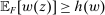 , we have
  . Combining this with the assumptions
  and
and  , we have

(“Only if” direction) Evidently, it suffices to prove the last statement of the proposition, since the conclusion of that sentence implies w is not scaling-dominated.
Assume none of (i)–(v) holds for w. Let  . Set
. Set 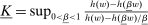 and
and 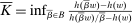 (which we define as ∞ if
  ). For
  , it must be that
 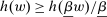 , otherwise (ii) would hold. Furthermore, this inequality is strict, otherwise (iii) would hold (unless
  but then (i) would hold). For any such
  , then
  is well-defined and is ≥1; hence
  . We are ensured
  , again by the negation of (iii). We also have that
  : either
  and
and  , or if B is nonempty and
  , property (v) holds. Finally, we know
  , otherwise (iv) would hold.
Choose any finite K such that  and
and  ; the previous paragraph ensures this is possible. Set the valuation
  . This is a valuation (i.e., its minimum value is 0) because w is grounded. Thus w is linear given v, with slope
  . For any
  , under contract βw, the worst-case expected profit is
  (or lower, if
  ). So, to establish that
  , it suffices to show
 (7)
(7) , this holds since
  and
and  is positive. For
  , this holds since
  and
and  is positive. If
  , then
  , unless
  , in which case
  . Thus (7) holds. Finally, for
  ,
,  , and we have
  for this case as well. Q.E.D.
Proof of Theorem 4.Let v be the valuation obtained by applying the last statement of Proposition 3 to  . Thus
  for some
  .
.
We hold v fixed. We will show that  , which is sufficient, since we already know that
  has the highest guarantee among linear contracts.
Let F be the distribution for which Responsiveness fails. Since  , it suffices to show that
 (8)
(8)
 . Applying the other part of the hypothesis of Responsiveness, and using
  , we have