Robust Screens for Noncompetitive Bidding in Procurement Auctions
Abstract
We document a novel bidding pattern observed in procurement auctions from Japan: winning bids tend to be isolated, and there is a missing mass of close losing bids. This pattern is suspicious in the following sense: its extreme forms are inconsistent with competitive behavior under arbitrary information structures. Building on this observation, we develop systematic tests of competitive behavior in procurement auctions that allow for general information structures as well as nonstationary unobserved heterogeneity. We provide an empirical exploration of our tests, and show they can help identify other suspicious patterns in the data.
1 Introduction
One of the key functions of antitrust authorities is to detect and punish collusive agreements. Although concrete evidence is required for successful prosecution, screening devices that flag suspicious firms help regulators identify such collusive agreements, and encourage members of existing cartels to apply for leniency programs.1 Correspondingly, an active research agenda has sought to build methods to detect collusion using naturally occurring market data (e.g., Porter (1983), Porter and Zona (1993, 1999), Ellison (1994), Bajari and Ye (2003), Harrington (2008)). This paper seeks to make progress on this research agenda by developing systematic tests of competitive behavior in procurement auctions under weak assumptions on the environment.
We begin by documenting a suspicious bidding pattern observed in first-price sealed-bid procurement auctions in Japan: the density of the bid distribution just above the winning bid is very low; there is a missing mass of close losing bids. These missing bids are related to bidding patterns observed among collusive firms in Hungary (Tóth et al. (2014)), Switzerland (Imhof, Karagök, and Rutz (2018)), and Canada (Clark, Coviello, and De Leveranoc (2020)). We establish that extreme forms of this pattern are inconsistent with competitive behavior under a general class of asymmetric information structures. Indeed, when winning bids are isolated, bidders can profitably deviate by increasing their bids. Expanding on this observation, we propose general tests of competitive behavior in procurement auctions that are robust, in the sense of holding under weak assumptions on the information structure and arbitrary unobserved heterogeneity.
Our data come from two sets of public works procurement auctions in Japan. The first data set contains information on roughly 7000 city-level auctions held between 2004 and 2018 by 14 different municipalities in Ibaraki prefecture and the Tohoku region of Japan. The second data set, analyzed by Kawai and Nakabayashi (2018), contains data on approximately 78,000 national-level auctions held between 2001 and 2006 by the Ministry of Land, Infrastructure, and Transportation. We are interested in the distribution of bidders' margin of victory and defeat. For every (bidder, auction) pair, we compute 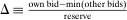 , the difference between the bidder's own bid and the most competitive bid among this bidder's opponents, divided by the reserve price. When
  , the bidder won the auction. When
  , the bidder lost. For both the municipal and national data sets, we document a missing mass in the distribution of Δ around
  . Our results clarify the sense in which this missing mass of close losing bids is suspicious, and help us identify other patterns in the data that are inconsistent with competition.
We analyze our data within a fairly general framework. A group of firms repeatedly participates in first-price procurement auctions. Players can observe arbitrary signals about one another, and bidders' costs and types can be correlated within and across periods. Importantly, we rule out dynamic considerations such as capacity constraints or learning by doing: we assume that current auction outcomes do not affect firms' future costs. Behavior is called competitive if it is stage-game optimal under the players' information.
Our first set of results establishes that, in its more extreme forms, the pattern of missing bids is not consistent with competitive behavior under any information structure. We exploit the fact that in any competitive equilibrium, firms must not find it profitable in expectation to increase their bids. This incentive constraint implies that with high probability the elasticity of firms' sample residual demand (i.e., the empirical probability of winning an auction at any given bid) must be bounded above by −1. This condition is not satisfied in portions of our data: because winning bids are isolated, the elasticity of sample residual demand is close to zero.
Our second set of results generalizes this test. In particular, we show how to exploit equilibrium conditions to derive bounds on the extent of noncompetitive behavior in our data. The bounds that we propose allow for very general information structures, contrasting with existing approaches that rely on specific assumptions such as independent private values (e.g., Bajari and Ye (2003)). As we show in our companion paper Ortner et al. (2020), antitrust policy based on tests that are robust to information structure cannot be exploited by cartels to enhance collusion. This addresses the concern articulated by Cyrenne (1999) and Harrington (2004) that data driven antitrust policies may end up facilitating collusion by providing cartel members a more effective threat point.
Our third set of results takes our tests to the data. We delineate how different moment conditions (i.e., different deviations) uncover different noncompetitive patterns. While missing bids suggest that a small increase in bids is attractive, we show that a moderate drop in bids (on the order of 2%) may also be attractive to bidders: it yields large increases in demand. In our data, downward deviations tend to be more informative about the competitiveness of auctions than upward deviations. In addition, upward and downward deviations are more informative together than separately. Finally, although failing our tests does not necessarily imply bidder collusion, we show that the outcomes of our tests are consistent with other proxy evidence for competitiveness and collusion. Bids that are high relative to the reserve price are more likely to fail our tests than bids that are low. Bids placed before an industry is investigated for collusion are more likely to fail our tests than bids placed after it is investigated for collusion. Altogether this suggests that, although our tests are conservative, they still have bite in practice.
Our paper relates primarily to the literature on cartel detection in auctions.2 Porter and Zona (1993, 1999) show that suspected cartel and noncartel members bid in statistically different ways. Bajari and Ye (2003) design a test of collusion based on excess correlation across bids. Conley and Decarolis (2016) propose a test of collusion in average-price auctions exploiting cartel members' incentives to coordinate bids. Chassang and Ortner (2019) propose a test of collusion based on changes in behavior around changes in the auction design. Kawai and Nakabayashi (2018) focus on auctions with rebidding, and exploit correlation in bids across stages to detect collusion.3 Marmer, Shneyerov, and Kaplan (2016) and Schurter (2020) design tests of collusion for English auctions and for first-price sealed bid auctions focusing on partial cartels. The tests that we propose relax assumptions imposed in previous work such as symmetry, independence, and private values (at the cost of reduced power), and can be used to detect both all-inclusive cartels and partial cartels.
More broadly, our paper relates to prior work that seeks to test for competitive behavior in other (nonauction) markets. Sullivan (1985) and Ashenfelter and Sullivan (1987) propose tests of whether firms behave as a perfect cartel, and apply these tests to the cigarette industry. Bresnahan (1987) and Nevo (2001) test for competition in the automobile and ready-to-eat cereal industries.4
Finally, our tests are also related to revealed preference tests seeking to quantify violations of choice theoretic axioms.5 Afriat (1967), Varian (1990), and Echenique, Lee, and Shum (2011) propose tests to quantify the extent to which a given consumption data set violates GARP. More closely related, Carvajal et al. (2013) propose a revealed preference test of the Cournot model.
2 Motivating Facts
Our first data set consists of roughly 7100 auctions for public works contracts held between 2004 and 2018 by municipalities located in the Tohoku region and Ibaraki prefecture of Japan. The auctions are sealed-bid first-price auctions with a publicly announced reserve price.6 The top panel of Table I reports summary statistics. The mean reserve price is 23.2 million yen, or about 230,000 USD, and the mean winning bid is 21.5 million yen. The mean number of bidders is 7.4. On average, a bidder in the data set participates in 23.3 auctions and wins 3.1 auctions.
|
Mean |
S.D. |
N |
||
|---|---|---|---|---|
|
City Auctions |
||||
|
By Auctions |
reserve price (mil. Yen) |
23.189 |
91.32 |
7111 |
|
lowest bid (mil. Yen) |
21.500 |
85.10 |
7111 |
|
|
lowest bid/reserve |
0.938 |
0.06 |
7111 |
|
|
#bidders |
7.425 |
3.77 |
7111 |
|
|
By Bidders |
participation |
23.29 |
43.58 |
2267 |
|
number of times lowest bidder |
3.14 |
6.22 |
2267 |
|
|
National Auctions |
||||
|
By Auctions |
reserve price (mil. Yen) |
105.121 |
259.58 |
78,272 |
|
lowest initial bid (mil. Yen) |
101.909 |
252.30 |
78,272 |
|
|
winning bid (mil. Yen) |
100.338 |
252.30 |
78,272 |
|
|
lowest bid/reserve |
0.970 |
0.10 |
78,272 |
|
|
winning bid/reserve |
0.946 |
0.10 |
78,272 |
|
|
ends in one round of bidding |
0.752 |
0.43 |
78,272 |
|
|
ends after one rebidding |
0.971 |
0.17 |
78,272 |
|
|
ends after two rebidding |
0.996 |
0.06 |
78,272 |
|
|
#bidders |
9.883 |
2.27 |
78,272 |
|
|
By Bidders |
participation |
26.40 |
94.61 |
29,670 |
|
number of times lowest bidder |
2.64 |
10.57 |
29,670 |
|
 the bid of firm i in auction a, and by
  the profile of bids by bidders other than i. We investigate the distribution of

 denotes the minimum bid from bidders other than i. The value
  represents the margin by which bidder i wins or loses auction a. If
  the bidder won, if
  she lost. Figure 1(a) plots the histogram and the density estimate of bid differences Δ aggregating over all firms and auctions in the sample. The mass of missing bids around 0 is clearly noticeable.
Distribution of bid-differences Δ over (bidder, auction) pairs. The dotted curves correspond to local (6th order) polynomial density estimates with bandwidth set to 0.0075.
Our second data set, studied in Kawai and Nakabayashi (2018), consists of roughly 78,000 auctions for construction projects held between 2001 and 2006 by the Ministry of Land, Infrastructure and Transportation in Japan (the Ministry). The auctions are sealed-bid first-price auctions with a secret reserve price. The average reserve price is 105.1 million yen, or about 1 million USD and the mean lowest bid is 101.9 million yen, which is 97.0% of the reserve price. Because the reserve price is secret, the lowest bid may be higher than the reserve price in which case there is rebidding. In that event, the reserve price remains secret to the bidders, but the lowest bid from the initial round is announced. There are at most two rounds of rebidding. If none of the bids are below the reserve price at the end of the second round of rebidding, the lowest bidder from the last round enters into a bilateral negotiation with the buyer. The auction concludes in the initial round of bidding about 75% of the time. The auction concludes after one round of rebidding in more than 97% of auctions and concludes after two rounds of rebidding in more than 99% of auctions. The mean number of participants is 9.9. For both data sets, all bids become public information after the auction. Figure 1(b) illustrates the distribution of bid-differences Δ for national auctions, where Δ is defined using first-round bids. The missing mass of bids around  is stark.
We point out another important (though less visually striking) feature of the densities plotted in Figure 1: the tails of the distribution taper off rapidly. This implies that much of the mass of Δ is concentrated within a relatively small interval around 0. For example, Δ lies between 0 and 0.02 for 50.0% of the losing bids in the city auctions and 25.6% of the losing bids in the national auctions. This implies that a drop in bids of 2% increases demand considerably (by 349% and 307%, resp.).7 Hence, while the missing bid pattern in Figure 1 suggests small increases in bids are profitable, the relatively large concentration of mass around  suggests that a small reduction in bids is also attractive (unless firms' profit margins are very small).
Correlation With Indicators of Collusion
Our analysis studies the extent to which the bidding patterns in Figure 1 are inconsistent with competitive behavior under arbitrary information structures. While noncompetitive behavior need not be collusive, we note that missing bids are in fact correlated with plausible indicators of collusion.
Since the goal of collusion is to elevate prices, we would expect to see suspicious bidding patterns in auctions with high bids. Figure 2 breaks down the auctions in Figure 1(b) by bid level: the figure plots the distribution of  for normalized bids
  below 0.8 (Panel (a)) and above 0.9 (Panel (b)). The mass of missing bids is considerably reduced in Panel (a). The tails of the distribution taper off more gradually in Panel (a).

Distribution of bid-difference Δ – national data. The dotted curves correspond to local (6th order) polynomial density estimates with bandwidth set to 0.0075.
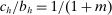
Figure 3 plots the distribution of  for participants of auctions held by the Ministry that were implicated by the Japanese Fair Trade Commission (JFTC). The JFTC implicated four bidding rings participating in auctions in our data: (i) firms installing electric traffic signs (Electric); (ii) builders of bridge upper structures (Bridge); (iii) prestressed concrete providers (PSC); and (iv) floodgate builders (Flood). The left panels in Figure 3 plot the distribution of Δ for auctions that were run before the JFTC started its investigation, and the right panels plot the distribution in the after period. In all cases except case (iii), the pattern of missing bids disappears after the JFTC launched its investigation. Interestingly, firms in case (iii) initially denied the charges against them (unlike firms in the other three cases), and seem to have continued colluding for some time (see Kawai and Nakabayashi (2018) for a more detailed account of these collusion cases).

Distribution of bid-difference Δ, before and after JFTC investigation.
What Does not Explain This Pattern
We end this section by arguing that missing bids are not explained by either the granularity of bids, or ex post renegotiation.
Figures 2 and 3 show that the pattern of missing bids in Figure 1 is not a mechanical consequence of the granularity of bids. If this was the case, we should see similar patterns across all bid levels, or before and after the JFTC investigations. In addition, Figure OC.2 in Appendix OC.1 in the Online Supplementary Material (Chassang et al. (2022)) plots the distribution of placebo statistic  , defined as the difference between bids and the most competitive other bid in bidding data from which each auction's lowest bid is excluded. The figure shows that the distribution of
  has no corresponding missing mass at 0.
Renegotiation could potentially account for missing bids by making apparent incentive compatibility issues irrelevant. However, in the auctions we study, contracts signed between the awarder and the awardee include a renegotiation provision which stipulates that renegotiated prices should be anchored to the initial bid. Specifically, if the project is deemed to require additional work, the government engineers estimate the costs associated with extra work. The firm is then paid  . This implies that a missing mass of Δ makes a small increase in bids profitable even taking into account the possibility of renegotiation. We provide further evidence on this point in Online Appendix OC.1: the missing bid pattern is present even in a subset of auctions for which we can ascertain that no price renegotiation took place.
3 Framework
3.1 The Stage Game
We consider a dynamic setting in which, at each period  , a buyer needs to procure a single project. In the main body of the paper, we assume that the auction format is a sealed-bid first-price auction with a public reserve price r, which we normalize to
  . Online Appendix OA extends the analysis to auctions with secret reserve prices and rebidding (as in the national data).
In each period t, a state  captures all relevant past information about the environment. Some elements of
  may be observed by the bidders at the time of bidding, but other elements may not be.8 All elements of
  are revealed to the bidders by the end of period t. Importantly,
  need not be observed by the econometrician. We assume that
  is an exogenous Markov chain (i.e., given any event E anterior to time t,
  ), but do not assume that there are finitely many states, that the chain is irreducible, or ergodic. The important assumption here is that by the end of each period t, bidders observe a sufficient statistic
  of future environments. Since
  evolves as an exogenous Markov process, we rule out intertemporal linkages between actions and payoffs.9 In practice, state
  may include the vector of distances between the project site and each of the firms, the vector of inputs specified in the construction plan, or the vector of current input prices. It may also include the current calendar date if there is seasonality in firms' costs. Lastly,
  may also include variables that are unknown to the bidders at the time of bidding, such as underground soil conditions. We do not assume that
  is observed by the econometrician.
In each period  , a set
  of bidders is able to participate in the auction, where N is the overall set of bidders. We think of this set of participating firms as those eligible to produce in the current period.10 The distribution of the set of eligible bidders
  can vary over time, but depends only on state
  . Participants discount future payoffs using a common discount factor
  .
.
Costs
Costs of production for eligible bidders  are denoted by
  . The bidder may or may not know its own costs at the time of bidding. The profile of costs
  may exhibit correlation across players and over time, but its distribution depends only on state
  . Because
  need not be finite-valued or ergodic, the distribution of costs can be arbitrarily different at every t. For example, if time t is included as part of state
  , then the distribution of costs can be different for every auction. All costs are assumed to be positive.
Information
In each period t, bidder i gets a signal  prior to bidding. The distribution of the profile of signals
  depends only on
  . Signals
  can take arbitrary values, including vectors in
  . Signals
  may reveal information about current state
  , bidder i's own costs
  , or the costs
  of other players. This allows our model to nest many informational environments, including private and common values, correlated values, asymmetric bidders, and asymmetric information.11 Since
  may not be finite valued or ergodic, our framework allows the distribution of signals
  to be different in every period t.
Bids and Payoffs
Each bidder  submits a bid
  . Profiles of bids are denoted by
  . We let
  denote bids from firms other than firm i, and define
 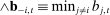 to be the lowest bid among i's competitors at time t. The procurement contract is allocated to the bidder submitting the lowest bid, at a price equal to her bid. Ties are broken randomly. Bids
  are publicly observed at the end of the auction.12
 obtains profits

 is the probability with which i wins the auction at time t.
3.2 Solution Concepts
 in period t takes the form
  . We let
  denote the set of all public histories. Our solution concept is perfect public Bayesian equilibrium (Athey and Bagwell (2008)). Because state
  is revealed by the end of each period, past play conveys no information about the private types of other players. As a result, we do not need to specify out-of-equilibrium beliefs. A perfect public Bayesian equilibrium consists only of a strategy profile
  , such that for all
  ,
,  maps public histories and payoff-relevant private signals to bids

Because our framework does not allow for intertemporal linkages between past actions and future payoffs, we can identify the class of competitive equilibria with the class of Markov perfect equilibria (Maskin and Tirole (2001)).
Definition 1. (Competitive strategy)We say that σ is Markov perfect if and only if  and
and  ,
,  depends only on
  .
.
We say that a strategy profile σ is a competitive equilibrium if it is a perfect public Bayesian equilibrium in Markov perfect strategies.
Competitive Histories
Our data sets involve many firms, interacting over an extensive timeframe. Realistically, an equilibrium may include periods in which (a subset of) firms collude and periods in which firms compete: we allow for both full and partial cartels. This leads us to define competitiveness at the history level.
Definition 2. (Competitive histories)Fix a common knowledge profile of strategies σ and a history  of player i. We say that player i is competitive at history
  if play at
  is stage-game optimal for firm i given the behavior of other firms
  .
.
We build up to our main inference problem, described in Section 6, in two steps. First, we show in Section 4 that even under general information structures, it is possible to use data to place restrictions on bidders' beliefs at the time of bidding. Second, we show in Section 5 that competitive behavior has testable implications, even under general incomplete information: the standard result that firms bid in the elastic part of the demand curve continues to hold for averages of demand. The results from Section 4 and Section 5 can be combined to construct a simple test of competition based on the idea that missing bids patterns are inconsistent with competition. Section 6 expands on these insights to obtain a probabilistic upper bound on the maximum share of histories consistent with competitive behavior.
4 Data-Driven Restrictions on Beliefs
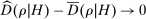
Because we make few assumptions on the environment, it is not obvious that bidding data can be used to test for competition. This section shows that as long as bidders play a perfect public Bayesian equilibrium, we can still place probabilistic constraints on the players' beliefs about their probability of winning.13 We show that in equilibrium the difference between realized demand (i.e.,  , for different values of b) and bidders' beliefs regarding demand is a martingale. Versions of the central limit theorem applying to sums of martingale increments imply that as the sample size grows, sample averages of demand must be close to the historical average of bidders' beliefs, even if those beliefs vary in a nonstationary way across histories.
 and all bids
  , player i's residual demand at
  is
is

 represents the bidders' beliefs regarding the probability of winning auction t for each possible bid
  she may place. Note that the conditioning variable
  in the expression includes the bidder's signal
  on which we have made very few assumptions. In particular, the distribution from which the signals
  are drawn can be different for each period t unlike in the conditional i.i.d. setting used in previous work.14 Indeed, bidders' beliefs can depend on public information and private signals that are unobserved to the econometrician. Still, it is possible to consistently estimate appropriately constructed averages of beliefs.
 . We denote by
  the average residual demand for histories in H and by
  its sample equivalent:
 (1)
(1) (2)
(2) denotes the cardinality of set H.
We now provide conditions on the set of histories H under which expression (2) consistently estimates (1).
Definition 3.We say that a set of histories H is adapted to the players' information if and only if the event  is measurable with respect to player i's information at time t, prior to bidding.
A subset H can be thought of as a selection of histories that satisfy certain criteria defined by the analyst. Definition 3 states that H is adapted if it is possible to check whether  satisfies the criteria needed for inclusion in H using only information available to bidder i at time t, prior to bidding.
Consider, for example, taking H to be the entire set of histories for a specific industry or location. The criteria for inclusion is that a particular history is for a specific industry or location. In this case, H is adapted because a bidder knows at the time of auction t that auction t is for a given industry or location. Hence, we do not need any information that the bidder does not know at the time of bidding to determine whether or not to include any such history in H.
Similarly, the set of histories in which a bidder bids a particular value is adapted since the bidder knows how she bids. In contrast, the set of histories in which a specific bidder wins the auction, or the set of histories in which the winning bid is equal to some value are not adapted.15
It is necessary for us to focus on adapted sets of histories to link realized demand and beliefs regarding demand (and payoffs). When we select a subset of histories H for data analysis, we are effectively evaluating outcomes under the conditioning event that  . When this event is in the information set of bidders at the time of bidding, then even conditional on this event, the differences between the bidders' beliefs and realizations of demand are zero, in expectation. This allows us to link realized outcomes to bidders' expectations, and obtain consistent estimates of the bidders' beliefs regarding demand and payoffs using realized data. This link disappears if we focus on a set of histories that is not adapted: the realized outcomes may be systematically different from the bidder's expectation at the time of bidding. For instance, if we focus on the set of histories such that a given bidder wins, then the bidder's realized demand under this conditioning event is 1, whereas the bidder's expected demand at the time of bidding will likely have been strictly below 1.
The notion of adaptedness formalizes the conditions on the sample selection rule such that sample averages consistently estimate bidder beliefs without introducing selection bias. In our empirical application, we take the set H to be histories in which the bids are above or below a particular value, histories in which a given firm places bids, etc. In each of these applications, the fact that we select the set of histories to be adapted guarantees that sample demand consistently estimates averages of bidders' beliefs.
Let  denote an upper bound on the number of participants in any auction.16
Proposition 1.Consider an adapted set of histories H. Under any perfect public Bayesian equilibrium σ, for any  ,
,

 as
as  .
.
In equilibrium, the sample residual demand conditional on an adapted set of histories converges to the historical average of bidders' beliefs about demand. This implies a confidence set 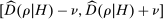 for the unobserved historical average of beliefs
  . We note that for simplicity, Proposition 1 uses nonasymptotic concentration results, and symmetric two-sided confidence sets. We revisit these choices with power in mind in Section 6, after introducing our main inference problem.17
What Drives Proposition 1 and When Can It Fail?
 ,
,
 (3)
(3) and
and  , that is, the fact that history
  satisfies the criteria for inclusion in H. This implies that the difference
  evolves like a martingale as
  grows. The Azuma–Hoeffding inequality yields Proposition 1.
 and the event
  are both known to the bidder at the time of bidding, the law of iterated expectations implies (3). Condition (3) would fail if set H was not adapted (in that case, being included in our analysis carries information unavailable to bidders at the time of bidding), or if bidders did not obtain feedback about past outcomes (in that case, the history of bids
  carries information unavailable to bidders at the time of bidding). For instance, imagine that bidders other than i experience a persistent drop in costs, so that they start bidding more aggressively than what firm i expected in period
  . If firm i gets no feedback about either bids or auction outcomes, it cannot update its beliefs and will systematically overestimate its demand at periods
  . Similarly, if we used a nonadapted set H, such as the set of bidding histories where bidder i wins, then (3) need not hold. Conditional on
  , the bidder wins the auction with probability 1, while bidder i's belief at the time of bidding can be strictly less than 1.
Condition (3) also clarifies the role of rational expectations. Outside expectation  and inside probability
  are indexed on the same stochastic process for bids generated by equilibrium σ. If bidders expected others' bids to be generated according to a strategy profile
  while actual bids are generated by strategy profile
  , then (3) need not hold. We note however that because past bids are observable, there exist prior-free solution concepts based on no-regret learning rules (Hart and Mas-Colell (2000)), which guarantee that a version of Proposition 1 would hold even without the rational expectations assumption.
5 Missing Bids Are Inconsistent With Competition
Our first main result shows that extreme forms of the pattern of bids illustrated in Figure 1 are inconsistent with competitive behavior.
Proposition 2.Let σ be a competitive equilibrium. Then
 (4)
(4) (5)
(5)
Proof.Consider a competitive equilibrium σ. Let

 . Let b denote the bid that bidder i places at history
  . Since b is an equilibrium bid, it must be that for all bids
  ,
,

 . Hence,
 (6)
(6) . This implies that for all
  ,
,

 ,
,  , and
, and  , we have that

 , this implies that

Proposition 2 extends the standard result that an oligopolistic competitor must price in the elastic part of her residual demand curve to settings with arbitrary incomplete information. Extreme forms of missing bids contradict Proposition 2: when the density of Δ at 0 is close to 0, the elasticity of demand is approximately zero.
As the proof highlights, this result exploits the fact that in procurement auctions, zero is a natural lower bound for costs.18 In contrast, for auctions where bidders are purchasing a good with positive value, there is no corresponding natural upper bound to valuations. One would need to impose an upper bound on values to establish similar results.
Because Proposition 1 allows us to obtain estimates (and confidence sets) of  and
and  , Propositions 1 and 2 together yield a simple test of whether or not an adapted set of histories H can be generated by a competitive equilibrium. This test holds under weak restrictions on the environment, and hence strengthens existing approaches that make specific assumptions such as symmetry, independent values, and private values (see, for instance, Bajari and Ye (2003)).
6 Bounding the Share of Competitive Histories
Proposition 2 derives testable implications of competition by using only the restriction that costs are nonnegative, and incentive compatibility conditions with respect to a single deviation: an increase in bids. In this section, we show how to obtain an upper bound on the share of competitive histories (or equivalently a lower bound on the share of noncompetitive histories) consistent with observed data. For this we exploit the information content of both upward and downward deviations, as well as possible restrictions on costs taking the form of markup constraints. Proposition 2 can be viewed as a special case of the results we present below. We also present asymptotic confidence sets that offer better power than Proposition 1. For simplicity, we assume that costs are private, and treat the case of common-value costs in Online Appendix OB.
We believe that estimating the share of noncompetitive histories, rather than just offering a binary test of competition, is practically important. Cartels are often partial, and regulators may want to prioritize more egregious cases. Measuring the prevalence of non-competitive behavior can help regulators gauge the magnitude of potential cartels and target investigations efficiently. This finer measure can also be used to track changes in cartel behavior over time. Finally, establishing that failures of noncompetitive behavior are not rare clarifies that bidders have plenty of opportunities to learn how to improve their bids. This suggests that failures to optimize stage-game profits are not merely errors.
6.1 Deviations, Beliefs, and Constraints
We begin by describing bidders' beliefs and the constraints they must satisfy: incentive compatibility constraints for competitive histories, markup constraints imposed by the analyst, and consistency with empirical demand (along the lines of Proposition 1).
Deviations and Beliefs
Take as given scalars  indexed by
  , such that
  and
and  for all
  . Each scalar
  parameterizes deviations
  from equilibrium bids
  .
.
 with equilibrium bid
  , deviation
  is associated with an expected demand
  corresponding to bidder i's belief that she would win the auction conditional on history
  and bid
  :
:

 associated with deviations
  is a vector in
  . The set of feasible beliefs
  is defined by
  .
. at those histories. It will be useful to consider the historical distribution
  of feasible beliefs
  induced by
  :
:

 is simply the (discrete) empirical measure defined on
  , which puts mass
  on realized beliefs and mass 0 on all other points. Distribution
  will be used to express averages of the history of beliefs
  as expectations under distribution
  . For instance, the average expected demand
  at different deviations can be expressed as
  . Indeed, for each
  ,
,

 is itself a random variable, depending on the realization of bidders' beliefs at the time of bidding. It is not observed by the econometrician.
Markup Constraints
 taking the form of markup constraints:
 (MKP)
(MKP) and
and  are minimum and maximum markups.19 Constraint (MKP) provides what we think is a transparent and convenient way for regulators to express intuitive subjective restrictions over the environment. Markups are simple familiar objects that analysts may have direct intuition or information about. In contrast, Bayesian priors over the underlying environment are high-dimensional objects for which little direct information is available.20,21 We discuss the impact of (MKP) on empirical inference in Section 7.
Incentive Compatibility Constraints
 is associated with feasible beliefs
  satisfying
 (IC)
(IC) ,
,
 (7)
(7) whenever
  , it follows that (7) is equivalent to22
 (8)
(8) (9)
(9) satisfying (
 satisfy

Empirical Consistency Constraints
The third constraint that beliefs must satisfy is that they must be consistent with data. Although we cannot pin down bidders' beliefs at individual histories, Proposition 1 implies probabilistic restrictions on average beliefs. With probability close to 1 as the number of histories gets large, the average expected demand at different deviations  must be close to its empirical counterpart
  , if H is adapted.
 we take as given a confidence set
  that covers the realized average expected demand
  with probability α. Set
  depends on realized bidding data alone, and satisfies

 , there exist confidence sets
  converging to the singleton set given by the historical mean beliefs
  when the sample size gets sufficiently large. For finite data however, the choice of confidence set
  will impact inference: some restrictions matter more than others to obtain upper bounds on the share of competitive histories. We describe the confidence sets
  used in our empirical implementation in Section 6.3 after presenting our main inference result.
6.2 Inferring a Bound on Competitive Histories
 , the share of histories
  in H that can be rationalized as competitive can be expressed as follows:

 is not observable, we can define a probabilistic upper bound
  :
:
 (P)
(P) (
( )
) consistent with empirical demand, that is, distributions μ such that
  .
.
Proposition 3.With probability greater than α,  .
.
For any threshold  , consider the test
  . Under the null that
  , test τ rejects the null with probability less than
  .
.
We remark that when we consider a single upward deviation and take  , the test
  reduces to a test of whether or not the elasticity of sample demand is higher than −1. Indeed, with a single upward deviation
  and
and  , (IC-MKP) reduces to
  . Hence, if
  , (IC-MKP) and
  cannot hold simultaneously for all histories
  whenever confidence set
  is a sufficiently small interval containing
  . In this sense, Proposition 2 can be viewed a special case of Proposition 3.23
The proof of Proposition 3 follows the logic of calibrated projection (Kaido, Molinari, and Stoye (2019)): a confidence set for an underlying parameter—here, the true average expected demand  —implies a confidence set for a function of the parameter—here, the share of competitive histories. Statistic
  is the upper bound of a confidence interval for underlying true parameter
  .
.
 is infinite dimensional, which makes program (P) computationally intractable. However, for each finite set
  , we can consider the following program:
 (Approx-P)
 .24 Our next result shows that, provided set
  is sufficiently dense within
  , the solution to (Approx-P) is approximately equal to
  .
.Consider a sequence  of finite subsets of
  , such that
  becomes dense in
  as n grows large. Denote by
  the solution to the approximate problem (Approx-P) associated with
  . The following result holds.
Lemma 1. .
.
A natural question is whether  is the tightest possible bound on the share of competitive histories. It is not. Program (P) exploits restrictions on beliefs imposed by (IC-MKP) and
  . We show in Appendix OB that when sample size is arbitrarily large, we would be exploiting all of the empirical content of equilibrium if we imposed demand consistency requirements
  conditional on all different values of bids and costs c (corresponding to the bidder's private information at the time of bidding). In practice, we find that this stretches both the limits of our data (in finite samples confidence levels drop as we seek to cover many conditional demands), and of bidder sophistication. Relying on a weaker set of optimality conditions makes our estimates more robust to partial failures of optimization, consistent with the critique of Fershtman and Pakes (2012).
6.3 Confidence Sets
 of feasible beliefs
  , taking the form of convex sets centered around empirical demand vector
  :
:
 (10)
(10) is a finite set of real vectors λ, parameters
  are given positive thresholds, and
  denotes the usual scalar product between vectors. Note that λ is a vector that is chosen by the researcher. For example, if we take λ to be a standard basis vector of the form
  , with the nth coordinate equal to 1, the corresponding inequality defines an upper bound on the nth element of d as
 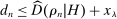 .
. (11)
(11) , it is sufficient to provide upper bounds for
  . As in Proposition 1, a nonasymptotic bound holds.
Lemma 2. (nonasymptotic coverage)For any adapted set of histories H, any vector  , and any threshold
  ,
,
 (12)
(12) .
.
Together with (11), Lemma 2 allows us to construct confidence sets  that have appropriate coverage for average expected demand
  . Note that we can set
  and
and  in expression (12) to obtain Proposition 1. The proof of Lemma 2 is very similar to that of Proposition 1. As in the case of Proposition 1, taking the set H to be adapted plays a crucial role.25
The attraction of bound (12) is that it is nonasymptotic. Unfortunately, it is also very conservative. For this reason, we provide less conservative asymptotic bounds relying on a central limit theorem for renormalized sums of martingale increments (see Billingsley (1995), Theorem 35.11).
 , so that
  grows with T. For any history
  , let
, let  denote the empirical demand at history
  . Recall that
  denotes bidder i's actual expected demand at history
  . We assume that
  and
and

 denote the set of bidding histories in H occurring prior to period t. Let
  denote the average empirical demand given bidding data available at time t. For any λ, we define

Lemma 3. (asymptotic coverage)For any adapted set of histories H, any vector  , and any threshold
  ,
,

 .
.
 that we use in our empirical investigation. Proofs for Lemmas 2 and 3 are provided in Online Appendix OD.
7 Empirical Findings
In this section, we estimate upper bounds on the share of competitive histories for the city-level and national-level auctions described in Section 2. Before reporting our findings, we discuss a few points regarding implementation and computation. We also give a brief discussion of how we address rebidding.
Implementation and Computation
We use confidence sets  of the form described by (10) and compute confidence levels using Lemma 3. In our application, we consider the bound
  corresponding to several different choices of deviations
  . When we consider a single downward, or a single upward deviation, we use
  and
and  , respectively. The key observation is that we apply negative coefficients to demand following deviations and positive coefficients to equilibrium demand. This implies lower bounds for demand (and therefore payoffs) after deviations, and upper bounds for demand (and therefore payoffs) in equilibrium.26 We pick thresholds
  to ensure a 98.33% confidence interval for each dot product
  , resulting in a 95% confidence level for
  .
.

 to ensure a 99% confidence interval for each dot product to obtain a 95% confidence level for
  .
.In practice, we solve problem (Approx-P) using the following parallelized algorithm for the case of  :
:
- 1. Draw 200 samples of 1000 tuples in
 using a seeded uniform distribution and sort each tuple in decreasing order.27 Each sample of 1000 points in
  corresponds to a finite subset
 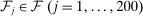 of feasible beliefs.
 - 2. For each sample
 , compute the solution
  to the associated problem (Approx-P). The solution
  is a
is a  vector of nonnegative numbers that sum to 1. Let
  denote the support of
  , truncated to cover 99% of the mass under
  by dropping belief vectors
  in order of ascending probability
  .28
.28 - 3. Set
 , and solve the associated (Approx-P) problem.
 - 4. Assess convergence by comparing the solution to that obtained starting from different random seeds up to 10−4.
Rebidding
City-level auctions use public reservation prices, and the results of Sections 5 and 6 apply directly. National-level auctions use secret reserve prices, and dealing with rebidding requires theoretical adjustments. As we explain in Online Appendix OA, incentive compatibility constraints for bid increases are essentially unchanged. For bid reductions, we need to assess losses in continuation values when (1) there is rebidding, (2) the bid reduction changes the lowest bid reported to bidders, thereby affecting their continuation information.29 We report bounds on the share of competitive histories computed under the assumption that changing the reported minimum bid reduces a bidder's continuation value by at most 50%.30
7.1 A Case Study
We first illustrate the mechanics of inference using bidding data from the city of Tsuchiura, located in Ibaraki prefecture. We do so by pooling bidding histories associated with auctions held prior to October 2009. Note that this set of histories is adapted. We select this city for two reasons: first, Chassang and Ortner (2019) provide evidence that there was collusion in auctions held prior to October 2009; second, the data turns out to be well suited to illustrate the information content of different incentive compatibility conditions.
We consider different combinations of deviations  , where by convention,
  is an infinitesimal downward deviation that amounts to breaking ties. The distribution of Δ and the deviations we consider (in dashed lines) are illustrated in Figure 4. The deviations are selected to deliver crisp illustrative results. We are specifically interested in illustrating the empirical content of individual deviations, as well as complementarities between upward and downward deviations.

Distribution of Δ for the city of Tsuchiura, 2007–2009.
A Single Upward Deviation
 . Under inference problem (P), we seek to maximize the share of histories such that demand
  satisfies (IC-MKP) subject to
  . For the case of a single upward deviation, (IC-MKP) reduces to


 is set to
  . An upward deviation is least profitable (and so the data is best explained) when costs are low. Aggregating across all histories, the IC constraints imply that
 (13)
(13) (14)
(14) small enough, (IC-MKP) and
  cannot be satisfied together for all histories
  . In auctions from Tsuchiura, a small upward deviation does not change a bidder's demand:
 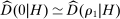 . This implies that (14) holds regardless of the value of M, and at least some fraction of histories in H must be deemed noncompetitive. Note that when
  , expression (13) reduces to a statement about the elasticity of demand, that is, Proposition 2.
The dotted line in Figure 5 corresponds to our estimate of the upper bound on the share of competitive histories based on Proposition 3 as a function of minimum markup m, using single upward deviation  . For these estimates and all the estimates we present below, we use Lemma 3 to construct confidence bounds and set tolerance
  so that our estimate is an upper bound for the true share of competitive histories with 95% confidence. We set
  .31 Since bounds based only on upward deviations do not depend on m, the dotted line in Figure 5 is constant at 0.87.

Share of competitive histories, Tsuchiura. Deviations {−0.02,0,0.0008}; maximum markup 0.5.
A Single Upward Deviation and Tied Bids
We now consider combining the upward deviation with an an infinitesimal downward deviation ( ). Any mass of tied bids is inherently noncompetitive since they create a meaningful benefit from reducing bids by the smallest possible amount. We note that tied bids are present in the data, but that their mass is small. Combining the upward deviation with an infinitesimal downward deviation, we estimate a 95% confidence bound on the share of competitive histories to be 0.86. This is illustrated as the horizontal dashed line in Figure 5. As the figure shows, the presence of ties has a very small impact on our estimate of the share of noncompetitive histories.
A Single Downward Deviation
 . For a single downward deviation, (IC-MKP) reduces to


 in the IC constraint (7), which means that the data patterns are best explained when costs are high.
 define a convex set. For
  small enough, (IC-MKP) and
  can be satisfied for all histories
  if and only if the mean empirical demand satisfies (IC-MKP):
 (15)
(15) , it follows that condition (15) always holds if m is close to zero. This is intuitive: for a sufficiently small margin, say
  , reducing bids by 2% results in losses for each auction (
 ). In contrast, if
 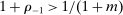 and demand increase
  is sufficiently large, then (15) does not hold and some share of histories must be considered noncompetitive.
The solid line in Figure 5 plots our estimate of the 95% confidence bound as a function of m. In this data, a 2% drop in prices leads to a 44 percentage-point increase in the probability of winning the auction, from  to
to 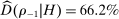 , almost tripling demand. Hence, as minimum markup m increases from 0, inequality (15) fails, implying that (IC) and
  cannot be solved together for all histories
  . Correspondingly, the bound in Figure 5 is equal to 1 for low values of m, and becomes less than 1 as m increases.32
Complementary Upward and Downward Deviations
Conditions (14) and (15) highlight that individual upward and downward deviations are rationalized as competitive by different costs. An upward deviation is least attractive when cost  is low. A downward deviation is least attractive when cost
  is large. Hence, upward and downward deviations are complementary from the perspective of inference. The dashed-dotted line in Figure 5 plots our bound on the share of competitive histories using all three deviations (
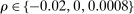 ). For all values of m, considering both upward and downward deviations leads to a tighter bound for the share of competitive histories than either upward or downward deviations alone (
 is 0.40 when
  ). The high costs needed to ensure that a downward deviation is not attractive also make upward deviations more attractive. Online Appendix OB.3 establishes this complementarity formally in a simple case.
7.2 Findings From Aggregate Data
We now apply our tests to the full set of auctions in each of our data sets, taking H as the set of histories corresponding to all municipal or national auctions. Clearly, H is adapted. Going forward, when applying the results of Section 6, we set  and use the fixed set of deviations
  for all data sets. Using a fixed set of deviations for all data sets is likely suboptimal for statistical power, but offers more transparency.33
Figure 6 shows our estimates of the 95% confidence bound on the share of competitive histories as a function of minimum markup m, for city and national auctions. The dotted line corresponds to the estimated bound when we set deviations  . The dashed and the solid lines correspond to estimates for deviations
  and
and 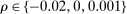 , respectively. In the case of national auctions, we use penalized incentive compatibility conditions accounting for rebidding detailed in Online Appendix OA.34 We note that upward deviations alone allow us to detect only a very small number of noncompetitive histories both in city-level auctions and in national-level auctions. One explanation for this is that looking at the full set of auctions causes us to mix competitive and noncompetitive histories, thereby weakening our ability to detect noncompetitive behavior.35 Correspondingly, our bound does not have much bite when we consider a single upward deviation and we take H to be the entire sample of auctions. Note that this does not mean that upward deviations are uninformative: especially in the case of national data, considering both upward and downward deviations can yield significantly tighter bounds on the share of competitive histories than either deviation alone.

Share of competitive histories, city, and national level data. Deviations {−0.02,0,0.001}; maximum markup 0.5.
7.3 Zeroing-in on Specific Firms
We now consider applying our tests to individual firms. As we highlight in Ortner et al. (2020), detecting noncompetitive behavior at the firm level helps reduce the potential side-effects of regulatory oversight. Specifically, it ensures that a cartel cannot use the threat of regulatory crackdown to discipline bidders.
For both city and national samples, we consider the 30 firms that participate in the most auctions in each data set. For each firm, we estimate a bound on the share of competitive histories taking H to be the set of histories corresponding to all instances in which the firm participates (set H is clearly adapted to the firm's information).
Panel (a) of Table II reports the results for firms active in the city sample. We order firms according to the number of auctions in which they participate. We report this number in column 2. Column 3 reports the share of auctions each firm wins as a fraction of the number of auctions in which the firm participates. Column 4 reports our estimates for the bound on the share of competitive histories using deviations 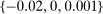 , minimum markup
  , and maximum markup
  . Panel (b) of Table II reports the corresponding results for firms in the national sample. Our bound is less than 1 for 18 firms for the city sample and 24 for the national sample.
|
(1) |
(2) |
(3) |
(4) |
|---|---|---|---|
|
Rank |
Participation |
Share won |
Share comp |
|
(a) City Data |
|||
|
1 |
347 |
0.19 |
0.88 |
|
2 |
336 |
0.21 |
0.86 |
|
3 |
299 |
0.08 |
0.98 |
|
4 |
293 |
0.05 |
1.00 |
|
5 |
290 |
0.14 |
1.00 |
|
6 |
287 |
0.20 |
1.00 |
|
7 |
269 |
0.14 |
0.94 |
|
8 |
268 |
0.09 |
0.97 |
|
9 |
262 |
0.12 |
1.00 |
|
10 |
259 |
0.18 |
0.90 |
|
11 |
252 |
0.12 |
0.97 |
|
12 |
241 |
0.12 |
0.95 |
|
13 |
239 |
0.16 |
0.93 |
|
14 |
238 |
0.09 |
0.99 |
|
15 |
227 |
0.11 |
0.97 |
|
16 |
226 |
0.12 |
0.99 |
|
17 |
225 |
0.08 |
0.96 |
|
18 |
223 |
0.12 |
0.98 |
|
19 |
220 |
0.07 |
1.00 |
|
20 |
218 |
0.08 |
1.00 |
|
21 |
211 |
0.07 |
1.00 |
|
22 |
210 |
0.14 |
0.95 |
|
23 |
209 |
0.17 |
0.93 |
|
24 |
204 |
0.15 |
1.00 |
|
25 |
203 |
0.11 |
0.98 |
|
26 |
199 |
0.06 |
1.00 |
|
27 |
190 |
0.12 |
1.00 |
|
28 |
189 |
0.06 |
1.00 |
|
29 |
188 |
0.16 |
0.94 |
|
30 |
187 |
0.08 |
1.00 |
|
(b) National Data |
|||
|
1 |
4044 |
0.17 |
0.84 |
|
2 |
3854 |
0.07 |
0.91 |
|
3 |
3621 |
0.12 |
0.85 |
|
4 |
2998 |
0.15 |
1.00 |
|
5 |
2919 |
0.06 |
0.92 |
|
6 |
2547 |
0.08 |
0.71 |
|
7 |
2338 |
0.07 |
0.74 |
|
8 |
2333 |
0.07 |
0.74 |
|
9 |
2328 |
0.04 |
0.95 |
|
10 |
2292 |
0.06 |
0.75 |
|
11 |
2237 |
0.08 |
0.90 |
|
12 |
2211 |
0.03 |
0.96 |
|
13 |
2015 |
0.09 |
0.76 |
|
14 |
1984 |
0.08 |
0.75 |
|
15 |
1727 |
0.07 |
1.00 |
|
16 |
1674 |
0.05 |
0.84 |
|
17 |
1661 |
0.03 |
0.94 |
|
18 |
1660 |
0.08 |
0.75 |
|
19 |
1589 |
0.07 |
0.79 |
|
20 |
1427 |
0.10 |
1.00 |
|
21 |
1393 |
0.06 |
0.86 |
|
22 |
1392 |
0.07 |
1.00 |
|
23 |
1370 |
0.04 |
0.92 |
|
24 |
1368 |
0.14 |
1.00 |
|
25 |
1353 |
0.05 |
0.80 |
|
26 |
1342 |
0.09 |
1.00 |
|
27 |
1337 |
0.04 |
0.87 |
|
28 |
1326 |
0.08 |
0.92 |
|
29 |
1291 |
0.06 |
0.86 |
|
30 |
1260 |
0.06 |
0.93 |
-
Note: 95% confidence bound on the share of competitive auctions for top thirty most active firms. The first column corresponds to the ranking of the firms and the second column corresponds to the number of auctions in which each firm participates. Column 3 shows the fraction of auctions that each of these firms wins. Column 4 present our 95% confidence bound on the share of competitive histories for each firm based on Proposition 3. For our estimates of column 5, we use deviations
 , minimum markup
  and maximum markup
  .
.
7.4 Consistency With Proxies for Collusion
We now show that our bounds on the share of competitive histories are consistent with proxies of collusive behavior. We consider different adapted subsets H associated with markers of collusion: whether or not the industry has been prosecuted for collusive practices, and whether bids are high compared to reserve prices.36 We then compute the associated estimates for the share of competitive histories.
Before and After Prosecution
As we noted in Section 2, the JFTC investigated firms bidding in four groups of national auctions during the period for which we have data: auctions labeled Bridges, Electric, Floods, and Prestressed Concrete. We now compute bounds on the share of competitive histories before and after investigation. We exclude the Bridge category because there are too few observations in the post-investigation sample to obtain a reliable confidence set (58 bids, versus more than 560 in the other industries).
Figure 7 shows our estimates of the 95% confidence bound on the share of competitive histories as a function of m, for the three remaining groups of firms. As above, we consider deviations  and set
  . For all three industries, we find that the share of competitive histories is higher after the investigation than before, consistent with the interpretation that collusion was more rampant before the investigation and less severe afterwards.37

Share of competitive histories, before and after JFTC investigation. Deviations {−0.02,0,0.001}; maximum markup 0.5.
High versus Low Bids
We now compare the estimates that we obtain when focusing on histories with low bids relative to high bids. Because collusion typically elevates prices, we expect the share of competitive histories to be higher for histories with low bids and vice versa. Specifically, we divide the city-level data into histories with high bids relative to the reserve price (i.e.,  ) and those with low bids (i.e.,
  ). Since the reserve price is known to bidders in the city auctions, these two sets of histories are adapted.
Figure 8 plots our estimates of the bound on the share of competitive histories for histories with high bids (solid line) and low bids (dotted line) for the city auctions. As before, we use deviations  and set
  . As the figure shows, the fraction of competitive histories is lower for histories with high bids. This is consistent with the fact that collusion increases bids.

Share of competitive histories by bid level, city data. Deviations {−0.02,0,0.001}; maximum markup 0.5.
8 Discussion
This paper develops tests of competitive bidding valid under general assumptions allowing for nonstationary costs and signals. In addition to the motivating observation that winning bids are isolated, we identify another suspicious pattern in the data: a 2% reduction in bids causes a large increase in demand.
Our tests are conservative: they can be passed by any firm that is bidding competitively under some information structure. Such caution is justified by the high direct and collateral costs of launching a formal investigation against noncollusive firms (Imhof, Karagök, and Rutz (2018)). In a companion paper building on the same framework (Ortner et al. (2020)), we identify another important property of such tests: antitrust investigation based on tests that are passed by any competitive firm does not generate new collusive equilibria. This addresses the concern that data-driven regulation may inadvertently enhance a cartel's ability to collude (Cyrenne (1999), Harrington (2004)). For these two reasons, we believe that our tests provide a sensible starting point for data-driven antitrust in public procurement.
The Online Appendices collect important extensions of our baseline framework: how to deal with secret reserve prices and rebidding; how to deal with common values; and how to construct money denominated metrics of noncompetitive behavior.
We conclude with a discussion of practical aspects of our tests: (i) firms' responses to antitrust oversight, (ii) the relation between the rejection of the test and collusion, (iii) non-collusive explanations for missing bids, and (iv) issues related to the implementation of our tests.
What if Firms Adapt?
Noncompetitive bidders may adapt to the screens used by antitrust authorities, reducing their efficacy. We show in a companion paper (Ortner et al. (2020)) that antitrust oversight based on tests that are robust to the information structure always reduces the set of enforceable collusive schemes available to cartels. That is, screens based on robust tests always make cartels worse off, even if firms know they are being monitored and adapt their play accordingly.
Moreover, we note that simple adaptive responses to our tests may themselves lead to suspicious patterns. For instance, collusive firms may adapt their play to our tests by “filling the gap” in the distribution of Δ to avoid generating the suspicious patterns in Figure 1.38 While such adaptive response would reduce the profitability of upward deviations by winning bidders, it would also make downward deviations by losing bidders more profitable, potentially also leading to patterns that would fail our tests.39
Rejection of the Test and Collusion
Our tests, which are aimed at detecting failures of competitive behavior, do not distinguish among the various reasons why a given data set may be inconsistent with competition. Failure to pass our test does not necessarily imply bidder collusion.40 However, findings from Section 7 show that rejection of our tests is in fact correlated with different markers of collusion. Indeed, in industries that were investigated for bid rigging, the fraction of competitive histories is lower before the investigation than after. The fraction of competitive histories is lower at histories at which bids are high relative to the reserve price. Altogether, this suggests that our test are sufficiently powered to flag cartels in practice.
Noncollusive Explanations
It is instructive to evaluate potential noncollusive explanations for the bidding patterns in our data. One possibility is that bidders are committing errors, say playing an ϵ-equilibrium of the game. This explanation is not entirely satisfactory for two reasons. First, the potential gains from downward deviations are not small, and bidders have many opportunities to learn. Second, natural models of erroneous play do not generate the patterns we see in the data. For instance, by adding noise on bids, quantal response equilibrium (McKelvey and Palfrey (1995)) would smooth out rather than enhance the pattern of missing bids.
Another possible explanation for the anomalous bidding patterns we note in the data is to take into account dynamic payoff consequences of winning an auction, through either capacity constraints, or learning by doing. A rapid analysis suggests that such dynamic considerations are unlikely to explain the data. Capacity constraints essentially correspond to an increase in the bidder's cost reflecting reduced continuation values. This increases the attractiveness of upward deviations. Similarly, learning-by-doing reduces the cost of accepting a project. This increases the attractiveness of downward deviations.
Practical Implementation
An important question for practical implementation concerns the choice of what set of histories H to apply our methods to. Besides the requirement that set H should be adapted, our analysis assumes that bidders take into account all the relevant information provided by past bidding data.41 Pooling data from competitive and noncompetitive environments may obscure noncompetitive bidding patterns, making it harder to reject the null of competition. The value of pooling data from different settings is that it potentially affords better power if noncompetitive behavior is broadly prevalent. In addition, separately analyzing subindustries raises multiple hypothesis testing concerns.
A second important aspect of practical implementation is the choice of deviations  being considered. As we have already noted, downward deviations are most binding when small drops in price lead to a large increase in demand. Upward deviations are most binding when relatively large increases in price cause relatively small drops in demand. Note that it may be difficult to estimate drops in demand for very small upward deviations (even if the empirical standard deviation of estimates is an exact 0). For that reason, we suggest that ρ should not be smaller (in absolute value) than the granularity of bids, that is, ρ should lie in the support of
  where
where  and
and  are adjacent (not necessarily winning) bids.
 prior to bidding. Components of
  that are observed to the bidder will be included in
  . For components of
  that are not observed, the bidder will form beliefs over their values based on the signal.
 .
.
 is consistently estimated by the empirical distribution of
  conditional on observables. In our setting, we cannot consistently estimate demand
  at each
  . We will only be able to obtain consistent estimates for averages of demand.
 to be a bound on the number of participants with histories in H in each auction.
 if they participate in an auction. In such a model, bidder i will only participate at time t and bid
  if
if  . Since
  , if bidder i chooses to participate, it must be that
  . Previous papers (e.g., Krasnokutskaya and Seim (2011)) have estimated that bid preparation costs can be substantial, between 2.2% and 3.9% of the engineer's cost estimate.
 , we set the left-hand side of (8) equal to +∞, −∞ or 0, depending on whether the numerator
  is positive, negative, or equal to zero.
 , then
  is simply a
  vector of nonnegative numbers that sum to 1. The objective function is
  and the constraint is
  . Note that both the objective function and the constraint are linear in μ.
 allow us to obtain bounds for demand (and for payoffs) following different deviations. For instance, when we consider a single downward deviation, we use
  . Hence, set
  includes beliefs
  satisfying
 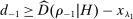 ,
,  and
and 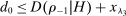 . The key observation is that we apply negative coefficients to demand following a deviation, and positive coefficients to equilibrium demand. This implies a lower bound for demand following a deviation, and an upper bound for equilibrium demand.
 if
if 
 are 0. This approach allows us to collect many good guesses using parallelized computations on relatively small samples, and then compute the solution associated with the union of these goods guesses.
 is very noticeable in Figure 1, the density at
  is not quite low enough at the aggregate level for upward deviations alone to have statistical power.
 .
.
 of demand
  is unbiased (and consistent provided the sample size of the data bidders do track becomes arbitrarily large), but our analysis underestimates its true standard error.
Appendix A: Proofs
Proof of Proposition 1.Let H be an adapted set of histories, and fix  . Recall that one auction happens at each time
  and that bidding outcomes are revealed in real time. For each time t, define

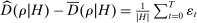 . Note further that, by the law of iterated expectations, for all public histories
  with
with  ,
,  . Hence,
  is a Martingale with respect to public histories
  . Since the absolute value of its increments
  is bounded above by
  , the number of bidders participating at time t with histories in H, the Azuma–Hoeffding inequality implies that for every
  ,
,

 , this implies that

Proof of Proposition 3.By assumption, constraint  is satisfied by the distribution of historical beliefs
  with probability greater than α. Whenever
  satisfies
  ,
,  is weakly larger than
  by construction. This implies that
  with probability greater than α.
Hence, if  , then with probability greater than α,
  , so that test
  rejects the null that
  with probability less than
  . Q.E.D.