Breaking Ties: Regression Discontinuity Design Meets Market Design
Abstract
Many schools in large urban districts have more applicants than seats. Centralized school assignment algorithms ration seats at over-subscribed schools using randomly assigned lottery numbers, non-lottery tie-breakers like test scores, or both. The New York City public high school match illustrates the latter, using test scores and other criteria to rank applicants at the city's screened schools, combined with lottery tie-breaking at the rest. We show how to identify causal effects of school attendance in such settings. Our approach generalizes regression discontinuity methods to allow for multiple treatments and multiple running variables, some of which are randomly assigned. The key to this generalization is a local propensity score that quantifies the school assignment probabilities induced by lottery and non-lottery tie-breakers. The utility of the local propensity score is demonstrated in an assessment of the predictive value of New York City's school report cards. Schools that earn the highest report card grade indeed improve SAT math scores and increase graduation rates, though by much less than OLS estimates suggest. Selection bias in OLS estimates of grade effects is egregious for screened schools.
1 Introduction
Large school districts increasingly use sophisticated centralized assignment mechanisms to match students to schools. In addition to producing fair and transparent admissions decisions, centralized assignment offers a unique resource for research on schools: the data these systems generate can be used to construct unbiased estimates of school value-added. This research dividend arises from the tie-breaking embedded in centralized assignment. Many school assignment schemes rely on the deferred acceptance (DA) algorithm, which takes as input information on applicant preferences and school priorities. In settings where seats are scarce, DA rations seats at over-subscribed schools using tie-breaking variables, thereby generating quasi-experimental variation in school assignment.
Many DA-implementing districts break ties with a uniformly distributed random variable, often described as a lottery number. Abdulkadiroğlu et al. (2017a) show that DA with lottery tie-breaking assigns students to schools as if in a stratified randomized trial. That is, conditional on preferences and priorities, the assignments generated by such systems are randomly assigned and therefore independent of potential outcomes. In practice, however, preferences and priorities, which we call applicant type, are too finely distributed for full nonparametric conditioning to be useful. We must therefore pool applicants of different types, while avoiding any omitted variables bias that might arise from the fact that type predicts outcomes.
The key to type pooling is the DA propensity score, defined as the probability of school assignment conditional on applicant type. In a mechanism with lottery tie-breaking, conditioning on the scalar DA propensity score is sufficient to make school assignment independent of potential outcomes. Moreover, the distribution of the scalar propensity score turns out to be much coarser than the distribution of types.1
This paper generalizes the propensity score to DA-based assignment mechanisms in which tie-breaking variables may include something other than randomly assigned lottery numbers. Selective exam schools, for instance, admit students with high test scores, and students with higher scores tend to have better achievement and graduation outcomes regardless of where they enroll. We refer to such scenarios as involving general tie-breaking.2 Matching markets with general tie-breaking raise challenges beyond those addressed in the Abdulkadiroğlu et al. (2017a) study of DA with lottery tie-breaking.
The most important complication raised by general tie-breaking arises from the fact that seat assignment is no longer independent of potential outcomes conditional on applicant type. This problem is intimately entwined with the identification challenge raised by regression discontinuity (RD) designs, which typically compare candidates for treatment on either side of a qualifying test score cutoff. In particular, non-lottery tie-breakers play the role of an RD running variable and are likewise a source of omitted variables bias. The setting of interest here, however, is more complex than the typical RD design: DA may involve many treatments, tie-breakers, and cutoffs.
A further barrier to causal inference comes from the fact that the propensity score in a general tie-breaking setting depends on the unknown distribution of non-lottery tie-breakers conditional on type. Consequently, the distribution of propensity scores under general tie-breaking may be no coarser than the underlying high-dimensional type distribution. When the score distribution is no coarser than the type distribution, score conditioning is pointless.
These problems are solved here by introducing a local DA propensity score that quantifies the probability of school assignment induced by a combination of non-lottery and lottery tie-breakers. This score is “local” in the sense that it is constructed using the fact that continuously distributed non-lottery tie-breakers are locally uniformly distributed. Combining this property with the (globally) known distribution of lottery tie-breakers yields a formula for the assignment probabilities induced by any DA match. Conditional on the local DA propensity score, school assignments are shown to be asymptotically randomly assigned. Moreover, like the DA propensity score for lottery tie-breaking, the local DA propensity score has a distribution far coarser than the underlying type distribution.
Our analytical approach extends Hahn, Todd, and Van der Klaauw (2001) and other pioneering nonparametric analyses of RD designs. We also build on the more recent local random assignment interpretation of nonparametric RD.3 The resulting theoretical framework allows us to quantify the probability of school assignment as a function of a few features of student type and tie-breakers, such as proximity to the admissions cutoffs determined by DA and the identity of key cutoffs for each applicant. By integrating nonparametric RD with Rosenbaum and Rubin (1983)'s propensity score theorem and large-market matching theory, our theoretical results provide a framework suitable for causal inference in a wide variety of applications.
The research value of the local DA propensity score is demonstrated through an analysis of New York City (NYC) high school report cards. This analysis aims to determine whether schools awarded “Grade A” on the district's school report cards are indeed high quality in the sense that they boost their students' achievement and improve other outcomes. Alternatively, the good performance of most Grade A students may reflect omitted variables bias. The distinction between causal effects and omitted variables bias is especially interesting in light of an ongoing debate over access to New York's academically selective schools, also called screened schools, which are especially likely to be graded A (see, e.g., Brody (2019) and Veiga (2018)). We identify the causal effects of Grade A school attendance by exploiting the NYC high school match. The NYC high school match employs a DA mechanism integrating non-lottery screened school tie-breaking with a common lottery tie-breaker at unscreened “lottery schools”. In fact, NYC screened high schools design their own tie-breakers based on middle school transcripts, test scores, interviews, and other factors.
The effects of Grade A school attendance are estimated using instrumental variables constructed from the school assignment offers generated by the NYC high school match. Specifically, our two-stage least squares (2SLS) estimators use assignment offers as instrumental variables for Grade A school attendance, while controlling for the local DA propensity score. The resulting estimates suggest that Grade A attendance boosts SAT math scores modestly and may increase high school graduation rates a little. But these Grade A effects are much smaller than the corresponding ordinary least squares (OLS) estimates.
We also compare 2SLS estimates of Grade A effects computed separately for NYC's screened and lottery schools. Perhaps surprisingly, this comparison shows the two sorts of schools to have similar (equally modest) causal effects. This finding therefore implies that OLS estimates showing a large Grade A screened school advantage are especially misleading, an important result in view of the ongoing debate over NYC school access and quality. Our estimates suggest that the public concern with screened school enrollment opportunities may be misplaced. On the methodological side, evidence of limited heterogeneity supports our assumption of constant treatment effects conditional on covariates.4
The next section shows how DA can be used to identify causal effects of school attendance. Section 3 illustrates key ideas through the example of a DA match with a single non-lottery tie-breaker. Section 4 derives a formula for the local DA propensity score in a matching market with general tie-breaking. This section also establishes a key identification result and derives a consistent estimator of the local propensity score. Section 5 uses these theoretical results to estimate causal effects of attending Grade A schools.5
2 Using Centralized Assignment to Eliminate Omitted Variables Bias
The NYC school report cards published from 2007 to 2013 graded high schools on the basis of student achievement, graduation rates, and other criteria. These grades were part of an accountability system meant to help parents choose high-quality schools. In practice, however, report card grades computed without extensive control for student characteristics reflect students' ability and family background as well as school quality. Systematic differences in student body composition are a powerful source of bias in school report cards. It is therefore worth asking whether a student who is randomly assigned to a Grade A high school indeed learns more and is more likely to graduate as a result.
We answer this question using instrumental variables derived from NYC's DA-based assignment of high school seats. The NYC high school match generates a single school assignment for each applicant as a function of applicants' preferences over schools, school-specific priorities, and a set of tie-breaking variables that distinguish between applicants who share preferences and priorities.6 Because they are a function of student characteristics like preferences and test scores, NYC assignments are not randomly assigned. We show, however, that conditional on the local DA propensity score, DA-generated assignment of seats at school s provides a credible instrument for enrollment at s. This result motivates a two-stage least squares (2SLS) procedure that instruments enrollment at any Grade A school with a dummy indicating DA-generated offers of a Grade A school seat.
Our identification strategy builds on the large-market “continuum” model of DA detailed in Abdulkadiroğlu et al. (2017a). The large-market model is extended here to allow for multiple and non-lottery tie-breakers. To that end, let  index schools, where
  represents an outside option. The set of applicants is the unit interval
  , where each applicant i is labeled by a number in the interval. The large-market model is large by virtue of this assumption. Seating is constrained by a capacity vector,
  , where
  is defined as the proportion of the unit interval that can be seated at school s. We assume
  , signifying a freely available outside option.
Applicant i's preferences over schools constitute a strict partial ordering,  , where
  means that i prefers school a to school b. Each applicant is also granted a priority at every school. For example, schools may prioritize applicants who live nearby or with currently enrolled siblings. Let
  denote applicant i's priority at school s, where
  means school s prioritizes i over j. We use
  to indicate that i is ineligible for school s. The vector
  records applicant i's priorities at each school. Applicant type is then defined as
  , that is, the combination of an applicant's preferences and priorities at all schools. Let
  denote the set of types, θ, that ranks s.
In addition to applicant type, DA matches applicants to seats as a function of a set of tie-breaking variables. Leaving DA mechanics for Section 4, at this point, it is enough to establish notation for DA inputs. Most importantly, our analysis of markets with general tie-breaking requires notation to keep track of tie-breakers. Let  index tie-breakers and let
  be the set of schools using tie-breaker v. We assume that each school uses a single tie-breaker. Scalar random variable
  denotes applicant i's tie-breaker v. Some of these are uniformly distributed lottery numbers. The profile of non-lottery
  used at schools ranked by applicant i is collected in the vector
  . Without loss of generality, we assume that ties are broken in favor of applicants with the smaller tie-breaker value. DA uses
  ,
,  , q, and the set of lottery tie-breakers for all i to assign applicants to schools.
We are interested in using the assignment variation resulting from DA to estimate the causal effect of  , a variable indicating student i's attendance at (or years of enrollment in) any Grade A school. Outcome variables, denoted
  , include SAT scores and high school graduation status. In a DA match like the one in NYC,
  is not randomly assigned, but rather reflects student preferences, school priorities, and tie-breaking variables, as well as decisions whether or not to enroll at school s when offered a seat there in the match. Selection bias arising from the process determining
  can be eliminated by an instrumental variables strategy that exploits the structure of matching markets.
 for the assignment of student i to a seat at school s. Because DA generates a single assignment for each student, a dummy for any Grade A assignment, denoted
  , is the sum of dummies indicating all assignments to individual Grade A schools.
  provides a natural instrument for
  . In particular, we estimate the effect of
  on
on  in the context of a linear constant-effects causal model that can be written as
 (1)
(1) (2)
(2) and
and  in these equations are functions of type and non-lottery tie-breakers, as well as a bandwidth,
  , that is integral to the local DA propensity score. In a constant-effects causal framework, observed outcomes are determined by
  , where
  is applicant i's potential outcome when
  is zero, modeled as
  .
. and
and  so that 2SLS estimates of β are consistent. Because (1) is seen as a model for potential outcomes rather than a regression equation, consistency requires that
  and
and  be uncorrelated. The relevant identification assumption can be written
 (3)
(3) , in a manner detailed below. Briefly, our main theoretical result establishes limiting local conditional mean independence of school assignments from applicant characteristics and potential outcomes, yielding (3). This result specifies
  and
and  to be easily-computed functions of the local propensity score and elements of
  .
.Abdulkadiroğlu et al. (2017a) derives the relevant DA propensity score for a scenario with lottery tie-breaking only. Lottery tie-breaking obviates the need for a bandwidth and control for components of  . Many applications of DA use non-lottery tie-breaking, however. The next section derives the propensity score for elaborate matches like that in NYC, which combines lottery tie-breaking with many school-specific non-lottery tie-breakers. The resulting estimation strategy integrates propensity score methods with both the nonparametric approach to RD (introduced by Hahn, Todd, and Van der Klaauw (2001)), and the local random assignment model of RD (discussed by Frolich (2007), Cattaneo, Frandsen, and Titiunik (2015), Cattaneo, Titiunik, and Vazquez-Bare (2017), and Frandsen (2017), among others). Our theoretical results can also be seen as generalizing nonparametric RD to allow for many treatments (in the form of schools), many running variables (in the form of tie-breakers), and many cutoffs.
3 Random Assignment from Non-Lottery Tie-Breaking in Serial Dictatorship
An analysis of a market with a single, shared non-lottery tie-breaker and no priorities illuminates key elements of our approach. DA in this case is called serial dictatorship. Like the local propensity score for DA in general, the serial dictatorship local score depends on only a handful of features, specifically, whether applicant i's tie-breaker is above, near, or below each of two key cutoffs. Conditional on this local propensity score, school assignment offers are randomly assigned in a limiting sense explained below.
Serial dictatorship is used in Boston, Chicago, and NYC to allocate seats at selective public exam schools.Order applicants by tie-breaker. Proceeding in order, assign each applicant to his or her most preferred school among those with seats remaining.
Because serial dictatorship relies on a single tie-breaker, notation for the set of non-lottery tie-breakers,  , can be replaced by a scalar,
  . As in Abdulkadiroğlu et al. (2017a), tie-breakers for individuals are modeled as stochastic, meaning they are drawn from a distribution for each applicant. For instance, when the tie-breaker is an exam score, the observed tie-breaker value is drawn from the distribution generated by retesting the applicant, just as a lottery number can be drawn repeatedly for each applicant. Although
  is not necessarily uniform, we assume that it is distributed with positive density over
  , with continuously differentiable cumulative distribution function,
  . These common support and smoothness assumptions notwithstanding, tie-breakers may be correlated with type, so that
  and
and  for applicants i and j are not necessarily identically distributed, though they are assumed to be independent of one another. The probability that type θ applicants have a tie-breaker below any value r is
  , where
  is
is  evaluated at r.
The serial dictatorship allocation is characterized by a set of tie-breaker cutoffs, denoted  for school s. For any school s that is filled to capacity,
  is given by the tie-breaker of the last (highest tie-breaker value) student assigned to s. Otherwise,
  , a non-binding cutoff reflecting excess capacity. Abdulkadiroğlu et al. (2017a) shows how to compute tie-breaker cutoffs in large-market models of the sort employed here.
Cutoffs are fudamental determinants of assignment rates, that is, of the probability of being seated at s. We say an applicant qualifies at s when they have a tie-breaker value that clears cutoff  . Under serial dictatorship, students are assigned to s if and only if they:
- qualify at s (since seats are assigned in tie-breaker order),
- fail to qualify at any school they prefer to s (since serial dictatorship assigns available seats at preferred schools first).
In large markets, moreover, cutoffs are constant, so the probability an individual applicant is seated at s is determined by the distribution of his or her tie-breaker alone.
3.1 The Serial Dictatorship Propensity Score
Which cutoffs matter for assignment probabilities? Under serial dictatorship, the assignment probability faced by an applicant of type θ at school s is determined by the cutoff at s and by cutoffs at schools preferred to s. By virtue of single tie-breaking, it is enough to know only one of the latter. In particular, an applicant who fails to clear the highest cutoff among those at schools preferred to s surely fails to do better than s. This leads us to define most informative disqualification (MID), a scalar parameter for each applicant type and school. MID tells us how the tie-breaker distribution among type θ applicants to s is truncated by disqualification at the schools type θ applicants prefer to s.
 (4)
(4) is then given by:
 (5)
(5) is zero when school s is ranked first, since
  is then empty. The second line in the definition of
  captures the fact that an applicant who ranks s second is seated there only when disqualified at the school they have ranked first, while applicants who rank s third are seated there when disqualified at their first and second choices, and so on. Qualification at these schools is determined by qualification at the school with the highest cutoff, that is, by
  . For example, applicants who fail to qualify at a school with a cutoff of 0.6 are disqualified at a school with cutoff 0.4.
 . This is the scenario sketched in the top panel of Figure 1, which illustrates the forces determining serial dictatorship assignment rates. Assignment rates when
  are given by the probability that


Assignment probabilities in serial dictatorship. Notes: This figure describes assignment probabilities for type θ applicants to school s. Probabilities are characterized as a function of τs, the cutoff at s, MIDθs, the most informative disqualification cutoff faced by type θ applicants to s, and the single tie-breaker distribution.
Proposition 1. (The Propensity Score in Serial Dictatorship)Suppose that seats in a large market are assigned by serial dictatorship. Assume that  is distributed with positive density over
  , with a continuously differentiable cumulative distribution function. Let
  denote the type-θ propensity score for assignment to s. For all schools s and type
  , we have

 , is given by the size of the group with
  between
  and
and  . This is

 , a scenario noted in Panel B of Figure 1. Thus, seats under serial dictatorship with lottery tie-breaking are randomly assigned as if in a randomized trial stratified by type, with treatment probability equal to
  .
.3.2 Serial Dictatorship Goes Local
With non-lottery tie-breaking, the serial dictatorship propensity score depends on the conditional distribution function,  evaluated at
  and
and  , rather than on cutoffs alone. This dependence leaves us with two econometric challenges. First,
  is unknown, so we can't compute the propensity score by repeatedly sampling from
  . Second,
  , is likely to depend on θ, so the score in Proposition 1 need not have coarser support than θ. This is in spite of the fact that many applicants with different values of θ share the same
  . Finally, although controlling for
  eliminates confounding from type, assignments are a function of tie-breakers as well as type. Confounding from non-lottery tie-breakers remains even after conditioning on
  .
.
These challenges are met here by focusing on assignment probabilities for applicants with tie-breaker realizations close to key cutoffs. Specifically, for each  , define an interval,
  , where parameter δ is a bandwidth analogous to that used for nonparametric RD estimation. The local propensity score treats the qualification status of applicants inside this interval as randomly assigned. This assumption is justified by the fact that, given continuous differentiability of tie-breaker distributions, non-lottery tie-breakers inside the bandwidth have a limiting uniform distribution as the bandwidth shrinks to zero.
The following proposition uses this fact to characterize the local serial dictatorship propensity score.
Proposition 2. (The Local Serial Dictatorship Propensity Score)Suppose seats in a large market are assigned by serial dictatorship and let  be any applicant characteristic other than type that is unchanged by school assignment.7 Finally, assume
  for all
  unless both cutoffs equal 1. Then,
  . Otherwise,


Proposition 2 describes a key conditional independence result: the limiting local probability of seat assignment in serial dictatorship takes on only three values and is unrelated to applicant characteristics. Note that the cases enumerated in the proposition (when  ) partition the tie-breaker line as sketched in the bottom panel of Figure 1. Applicants with tie-breaker values above the cutoff at s are disqualified at s and so cannot be seated there, while applicants with tie-breaker values below
  are qualified at a school they prefer to s and so will be seated elsewhere. Applicants with tie-breakers strictly between
  and
and  are surely assigned to s. Finally, type θ applicants with tie-breakers near either
  or the cutoff at s are seated with probability approximately equal to
  . Nearness in this case means inside the interval defined by bandwidth δ.
The driving force behind Proposition 2 is the assumption that the tie-breaker distribution is continuously differentiable. In a shrinking window, the tie-breaker density therefore approaches that of a uniform distribution, so the limiting qualification rate is  (see Abdulkadiroğlu et al. (2017b) or Bugni and Canay (2018) for proof of this claim). The assumption of a continuously differentiable tie-breaker distribution is analogous to the continuous running variable assumption invoked in Lee (2008) and to a local smoothness assumption in Dong (2018). Continuity of tie-breaker distributions implies that the conditional expectation functions of potential outcomes given running variables are continuous at cutoffs. The latter condition features in Hahn, Todd, and Van der Klaauw (2001) and much of the subsequent theoretical analysis of nonparametric identification in RD. We favor the stronger continuity assumption because the implied local random assignment provides a scaffolding for construction of assignment probabilities in more elaborate matching scenarios.8
4 The Local DA Propensity Score
Many school districts assign seats using a version of student-proposing DA, which can be described like this:
Each applicant proposes to his or her most preferred school. Each school ranks these proposals, first by priority, then by tie-breaker within priority groups, provisionally admitting the highest-ranked applicants in this order up to its capacity. Other applicants are rejected.
Each rejected applicant proposes to his or her next most preferred school. Each school ranks these new proposals together with applicants admitted provisionally in the previous round, first by priority and then by tie-breaker. From this pool, the school again provisionally admits those ranked highest up to capacity, rejecting the rest
The algorithm terminates when there are no new proposals (some applicants may remain unassigned).
Different schools may use different tie-breakers. For example, the NYC high school match includes a diverse set of screened schools. These schools admit applicants using school-specific tie-breakers that are derived from interviews, auditions, or GPA in earlier grades, as well as test scores. The NYC match also includes many unscreened schools, referred to here as lottery schools, that use a uniformly distributed lottery number as tie-breaker. Lottery numbers are distributed independently of type and potential outcomes, but non-lottery tie-breakers like entrance exam scores almost certainly depend on these variables.
4.1 Assumptions and Theorem
We assume the match of interest involves V distinct tie-breakers, adopting the convention that tie-breaker indices are ordered so that lottery tie-breakers come first. Specifically, let  index U lottery tie-breakers, where
  . Each lottery tie-breaker,
  for
for  , is uniformly distributed over
  . Non-lottery tie-breakers are indexed by
  . The set of tie-breakers is restricted as follows:
Assumption 1.
- (i) For any tie-breaker indexed by
 and applicants
  , tie-breakers
  and
and  are independent, though not necessarily identically distributed.
 - (ii) The joint distribution of non-lottery tie-breakers,
 for applicant i, is continuously differentiable with positive density over
  .
.
Assumption 1 implies that the tie-breaker distribution for any subset of applicants is continuously differentiable. This follows from Assumption 1 since the integral of continuously differentiable distributions is also continuously differentiable.
 be a function that returns the index of the tie-breaker used at school s. By definition,
  . To combine applicants' priority status and tie-breaking variables into a single number for each school, we define applicant position at school s as

Cutoffs are also generalized to incorporate priorities; these DA cutoffs are denoted  . For any school s that ends up filled to capacity,
  is given by
  . Otherwise, we set
  to indicate that s has slack (recall that K is the lowest possible priority for eligible applicants).
 (6)
(6) is constant. DA-determined school assignment rates are therefore determined by the distribution of stochastic tie-breakers evaluated at fixed school cutoffs. Condition (6) nests our characterization of seat assignment under serial dictatorship since we can set
  for all applicants and use a single tie-breaker to determine position. Statement (6) then says that
  and
and  for applicants with
  .
. and defined as
  , the integer part of the DA cutoff. Conditional on rejection by all preferred schools, applicants to s are assigned s with certainty if
  , that is, if they clear marginal priority. Applicants with
  have no chance of finding a seat at s. Applicants for whom
  are marginal: these applicants are seated at s when their tie-breaker values fall below tie-breaker cutoff
  . The tie-breaker cutoff can therefore be written as the decimal part of the DA cutoff:

 , so their
  if and only if
  .
. , as follows:


Elements of  for unscreened schools are a function only of the partition of types determined by marginal priority. For screened schools, however, the classification vector
  also encodes the proximity of applicant tie-breakers to cutoffs. Never-seated applicants to s cannot be seated there, either because they fail to clear marginal priority at s or because they are too far above the cutoff when s is screened. Always-seated applicants to s are assigned s for sure when they cannot do better, either because they clear marginal priority at s or because they are well below the cutoff at s when s is screened. Finally, conditionally-seated applicants to s are randomized marginal priority applicants. Randomization is by lottery number when s is a lottery school or by non-lottery tie-breaker within the bandwidth when s is screened.

 and
and  , where
  for each s.
  describes assignment probabilities as a function of type and cutoff proximity determined by bandwidth value δ. With this notation in hand, the local DA propensity score is given by the limit

As in Proposition 2, our formal characterization of  assumes tie-breaker cutoffs are distinct:
Assumption 2. for all
  unless
  .
.
 also requires an extension of most informative disqualification to a general tie-breaking regime and DA with priorities. To that end, the set of schools θ prefers to s is partitioned by by defining
  for each tie-breaker, v. We then have

 quantifies the extent to which qualification for seats in the set of schools that type θ applicants prefer to s and that use tie-breaker
  truncates the tie-breaker distribution among applicants contending for seats at s.
 for type θ applicants in the bandwidth around this cutoff.
 and
and  to compute disqualification rates at all schools preferred to s. We break this into two pieces: variation generated by screened schools and variation generated by lottery schools. As the bandwidth shrinks, the limiting disqualification probability at screened schools in
  converges to
 (7)
(7) is
is
 (8)
(8)To recap: the local DA score for type θ applicants is determined in part by the screened schools θ prefers to s. Relevant screened schools are those determining  , and at which applicants are close to tie-breaker cutoffs. The variable
  counts the number of tie-breakers involved in such close encounters. Applicants drawing screened school tie-breakers close to
  for some
  face qualification rates of 0.5 for each tie-breaker v. Since screened school disqualification is locally independent over tie-breakers, the term
  computes the probability of not being assigned a screened school preferred to s. Likewise, since the qualification rate at preferred lottery schools is
  , the term
  computes the probability of not being assigned a lottery school preferred to s.
The following theorem combines these in a formula for the local DA propensity score:
Theorem 1. (The Local DA Propensity Score With General Tie-breaking)Suppose seats in a large market are assigned by DA with tie-breakers indexed by v, and that Assumptions 1 and 2 hold. For all schools s, applicant types θ, tie-breaker classifications T, and values of w in the support of  (as defined in Proposition 2), we have

 , or (b)
  ,
,  . Otherwise,
 (9)
(9)Theorem 1, proved in the Appendix, starts with a scenario where applicants to s are either disqualified there or assigned to a preferred school for sure. In this case, we need not worry about whether s is a screened or lottery school. In other scenarios where applicants are surely qualified at s, the probability of assignment to s is determined entirely by disqualification rates at preferred screened schools and by truncation of lottery tie-breaker distributions at preferred lottery schools. These forces combine to produce the first line of (9). The conditional assignment probability at any lottery s, described on the second line of (9), is determined by the disqualification rate at preferred schools and the qualification rate at s, where the latter is given by  (to see this, note that
  includes the term
  in the product over lottery tie-breakers). Similarly, the conditional assignment probability at any screened s, on the third line of (9), is determined by the disqualification rate at preferred schools and the qualification rate at s, where the latter is given by 0.5.
The theorem covers the non-lottery tie-breaking serial dictatorship scenario sketched in the previous section. With a single non-lottery tie-breaker,  . When
  or
or  for some
  , the local propensity score at s is zero. Otherwise, suppose
  for all
  , so that
  . If
. If  , then the local propensity score is 1. If
  , then the local propensity score is 0.5. Suppose, instead, that
  for some
  , so that
  . In this case,
  because cutoffs are distinct (Assumption 2). If
  , then the local propensity score is 0.5. Appendix B in the Supplemental Material illustrates the theorem in other scenarios.
 denote the set of Grade A schools. Because DA generates a single offer, the local DA propensity score for assignment to any Grade A school, denoted
  , is
, is
 (10)
(10)
 . We then have the following corollary to Theorem 1:
Corollary 1. (Identification)Suppose Assumptions 1 and 2 hold and that Grade A causal effects are given by a constant, β, so that observed outcomes are determined by  . Assume that
  affects
  solely by changing
  , so that Theorem 1 holds for
  . Assume also that there exists some
  such that
  , where the conditional expectations are assumed to exist. Then β is uniquely determined by the joint distribution of
  .
.
This result is a consequence of the fact that, conditional on the local propensity score characterized in Theorem 1, Grade A assignment is independent of applicant characteristics. The corollary postulates that potential outcomes are unchanged by school assignment, an exclusion restriction which, in combination with Theorem 1, implies assignment is independent of  as well. Therefore, assuming the probability of Grade A assignment falls strictly between zero and 1 and that the resulting offer variation changes Grade A enrollment, a simple instrumental variables estimand gives the causal effect of Grade A attendance on outcome variable,
  .
.
4.2 Score Estimation
Theorem 1 characterizes the theoretical probability of school assignment in a large market with a continuum of applicants. In reality, of course, the number of applicants is finite and propensity scores must be estimated. We show here that, in an asymptotic sequence that increases market size with a shrinking bandwidth, a sample analog of the local DA score described by Theorem 1 converges to the corresponding local score for a finite market. Our empirical application establishes the relevance of this asymptotic result by showing that applicant characteristics are balanced by assignment status conditional on estimates of the local DA propensity score.
The asymptotic sequence for the estimated local DA score works as follows: randomly sample N applicants from a continuum economy with a fixed vector of school capacities,  , giving the proportion of N seats that can be seated at s. We observe realized tie-breaker values for each applicant, along with applicant type, but not the underlying distribution of non-lottery tie-breakers. The (finite) set of schools is unchanged along this sequence.
 and run DA with these applicants and schools. Let
  be the realized cutoff at school s. We consider the limiting behavior of an estimator computed using the estimated cutoffs,
  , the corresponding
  for an applicant of of type
  , and marginal priorities generated by this single realization (note that
  is an estimated quantity). Also, given a bandwidth
  , we compute
  for each i and s, collecting these in classification vector
  . These statistics then determine

 , is constructed by plugging these ingredients into the formula in Theorem 1. That is, if (a)
  , or (b)
  , then
  . Otherwise,
 (11)
(11)

 , consider the true local DA score for a finite market of size N. This is
 (12)
(12) is the expectation induced by the joint tie-breaker distribution for applicants in the finite market. This quantity is defined by fixing the distribution of types and the vector of proportional school capacities, as well as market size.
  is then the limit of the average of
  across infinitely many tie-breaker draws in ever-narrowing bandwidths for this finite market. Because tie-breaker distributions are assumed to have continuous density in the neighborhood of any cutoff, the finite-market local propensity score is well-defined for any positive δ.
For all  and classification vectors
  , we are interested in the gap between the estimator
  and the true local score
  as N grows and
  shrinks. We aim to show that
  converges to
  in our asymptotic sequence. This result uses a regularity condition:
Assumption 3. (Rich Support)In the population continuum market, for every school s and every priority ρ held by a positive mass of applicants who rank s, the proportion of applicants i with  who rank s first is also positive.
Convergence of  is formalized in the theorem below:
Theorem 2. (Consistency of the Estimated Local DA Propensity Score)In the asymptotic sequence described above, and maintaining Assumptions 1–3, the estimated local DA propensity score  is a consistent estimator of
  in the following sense: Take any sequence such that
  and
and  as
as  . For any type θ and tie-breaker classification T, consider applicants with
  and
and  . Then, for all schools s,

Theorem 2 is proved in Appendix C in the Supplemental Material. The proof shows that  converges to
  , and so
  converges to
  as well as to
  .
.
4.3 Treatment Effect Estimation

 (13)
(13) (14)
(14) and the set of parameters denoted
  and
and  provide saturated control for the local propensity score. As detailed in the next section, functions
  and
and  implement local linear control for screened school tie-breakers for the set of applicants to these schools with
  . Linking this with the empirical strategy sketched at the outset, equation (13) is a version of of equation (1) that sets

 defined similarly.
Our score-controlled instrumental variables estimator adapts a simple procedure discussed by Calonico et al. (2019). Specifically, using a mix of simulation evidence and theoretical reasoning, Calonico et al. (2019) argues that additive linear control for covariates in a local linear regression model requires fewer assumptions and is likely to have better finite sample behavior than more elaborate estimators (e.g., allowing covariate controls to change at cutoffs). The covariates of primary interest to us are dummies for values in the support of the Grade A local propensity score.10
Note that saturated regression-conditioning on the local propensity score eliminates applicants with estimated score values of zero or 1. This is apparent from an analogy with a fixed-effects panel model. In panel data with multiple annual observations on individuals, estimation with individual fixed effects is equivalent to estimation after subtracting person means from regressors. Here, the “fixed effects” are coefficients on dummies for each possible score value. When the score value is 0 or 1 for applicants of a given type, assignment status is constant and observations on applicants of this type drop out. We therefore say an applicant has Grade A risk when  . The sample with risk contains applicants contributing to parameter estimation in models with saturated score control.
Propensity score conditioning facilitates control for applicant type in the sample with risk. This is because local propensity score conditioning yields considerable dimension reduction relative to full-type conditioning, as we would hope. The 2014 NYC high school match, for example, involved 52,208 applicants of 47,153 distinct types (among those with baseline test scores and other covariates). Of these, 42,527 types listed at least one Grade A school on their application to the high school match. By contrast, the estimated local propensity score for Grade A school assignment takes on only 1,843 values.
5 A Brief Report on NYC Report Cards
5.1 Doing DA in the Big Apple
Since the 2003–2004 school year, the NYC Department of Education (DOE) has used DA to assign rising ninth graders to high schools. Many high schools in the match host multiple programs, each with their own admissions protocols. Applicants are matched to programs rather than schools. Each applicant for a ninth grade seat can rank up to twelve programs. All traditional public high schools participate in the match, but charter schools and NYC's specialized exam high schools have separate admissions procedures.11
The NYC match is structured like the general DA match described in Section 4: lottery programs use a common uniformly distributed lottery number, while screened programs use a variety of non-lottery tie-breaking variables. Screened tie-breakers are mostly distinct, with one for each school or program, though some screened programs share a tie-breaker. In any case, our theoretical framework accommodates all of NYC's many tie-breaking protocols.12
Our analysis uses Theorems 1 and 2 to compute propensity scores for programs rather than schools since programs are the unit of assignment. For our purposes, a lottery school is a school hosting any lottery program. Other schools are defined as screened.13
In 2007, the NYC DOE launched a school accountability system that graded schools from A to F. This mirrors similar accountability systems in Florida and other states. NYC's school grades were determined by achievement levels and, especially, achievement growth, as well as by survey- and attendance-based features of the school environment. Growth looked at credit accumulation, Regents test completion and pass rates; school performance measures were derived mostly from four- and six-year graduation rates. Some schools were ungraded. Figure 2 reproduces a school progress report from this era.14

A Sample NYC school report card.
The 2007 grading system was controversial. Proponents applauded the integration of multiple measures of school quality while opponents objected to the high-stakes consequences of low school grades, such as school closure or consolidation. Rockoff and Turner (2011) provides a partial validation of the grading system by showing that low grades seem to have sparked school improvement. In 2014, the NYC DOE replaced the 2007 scheme with school quality measures placing less weight on test scores and more weight on curriculum characteristics and subjective assessments of teaching quality. The relative merits of the old and new systems continue to be debated.
The results reported here use application data from the 2011–2012, 2012–2013, and 2013–2014 school years (students in these application cohorts enrolled in the following school years). Our sample includes first-time applicants seeking ninth grade seats, who submitted preferences over programs in the main round of the NYC high school match. We obtained data on school capacities and priorities, lottery numbers, and screened school tie-breakers, information that allows us to replicate the match. Details related to match replication appear in Appendix D in the Supplemental Material.15
Students at Grade A schools have higher average SAT scores and higher graduation rates than do students at other schools. Such differences feature in popular accounts of socioeconomic differences in school access (see, e.g., Harris and Fessenden (2017) and Disare (2017)). Grade A students are also more likely than students attending other schools to be deemed “college- and career-prepared” or “college-ready.”16 These and other school characteristics appear in Table I, which reports statistics separately by report card grade and admissions regime. Achievement gaps between students attending screened and lottery Grade A schools are especially large, likely reflecting selection bias induced by test- and GPA-based screening.
|
Grade A schools |
Grade B–F Schools |
Ungraded Schools |
|||
|---|---|---|---|---|---|
|
All |
Screened |
Lottery |
|||
|
(1) |
(2) |
(3) |
(4) |
(5) |
|
|
Panel A. Average Performance Levels |
|||||
|
SAT Math (200–800) |
531 |
606 |
481 |
464 |
440 |
|
SAT Reading (200–800) |
522 |
587 |
479 |
465 |
449 |
|
Graduation rate |
0.83 |
0.92 |
0.77 |
0.70 |
0.47 |
|
College- and career-prepared |
0.65 |
0.84 |
0.54 |
0.39 |
0.27 |
|
College-ready |
0.59 |
0.82 |
0.45 |
0.34 |
0.24 |
|
Panel B. School Characteristics |
|||||
|
Black |
0.20 |
0.12 |
0.25 |
0.32 |
0.39 |
|
Hispanic |
0.35 |
0.26 |
0.41 |
0.40 |
0.43 |
|
Special Education |
0.12 |
0.06 |
0.16 |
0.17 |
0.27 |
|
Free or Reduced Price Lunch |
0.68 |
0.55 |
0.76 |
0.77 |
0.75 |
|
In Manhattan |
0.27 |
0.49 |
0.12 |
0.16 |
0.28 |
|
Number of grade 9 students |
420 |
430 |
414 |
413 |
86 |
|
Number of grade 12 students |
374 |
413 |
348 |
351 |
53 |
|
High school size |
1596 |
1700 |
1527 |
1509 |
426 |
|
Inexperienced teachers |
0.11 |
0.10 |
0.12 |
0.11 |
0.28 |
|
Advanced degree teachers |
0.53 |
0.59 |
0.49 |
0.50 |
0.30 |
|
New school |
0.00 |
0.00 |
0.01 |
0.00 |
0.21 |
|
School-year observations |
355 |
119 |
236 |
694 |
715 |
- Note: This table reports student-weighted average performance levels and characteristics of NYC high schools. Panel A shows performance measures for cohorts enrolled in ninth grade in 2012–2013, 2013–2014, and 2014–2015. Panel B shows school characteristics for these years. A screened school is defined as any school without lottery programs. Inexperienced teachers have 3 or fewer years of experience; advanced degree teachers have a master's or higher degree. Specialized and charter high schools admit applicants in a separate match and are coded as screened and lottery schools, respectively.
Screened Grade A schools have a majority white and Asian student body, the only group of schools described in Table I to do so (the table reports shares Black and Hispanic). These schools are also over-represented in Manhattan, a borough that includes most of New York's wealthiest neighborhoods (though average family income is higher on Staten Island). Excepting ungraded (and mostly newer) schools, teacher experience is similar across school types, while screened Grade A schools have somewhat more teachers with advanced degrees.
The first column of Table II describes the roughly 180,000 ninth graders enrolled in the 2012–2013, 2013–2014, and 2014–2015 school years. These statistics can be compared with the statistics in column 2, which describe the approximately 47,000 students enrolled in a Grade A school (including students enrolled in the Grade A schools assigned outside the match). Grade A students have higher baseline scores than the general population of ninth graders and are less likely to be Black or Hispanic (Baseline scores are from tests taken in sixth grade and standardized to the population of test-takers). The 153,000 eighth graders who applied for ninth grade seats are described in column 3 of the table. Roughly 130,000 listed a Grade A school for which seats are assigned in the match on their application form and a little over a third of these were offered a Grade A seat.17 Match participants have baseline scores above the overall district mean. As can be seen by comparing columns 3 and 4 in Table II, however, the average characteristics of Grade A applicants are mostly similar to those of the entire applicant population.
|
Ninth Grade Students |
Applicants for Ninth Grade Seats |
|||||
|---|---|---|---|---|---|---|
|
All |
Enrolled in Grade A |
All |
Listed Grade A |
Enrolled in Grade A |
At Risk at Grade A |
|
|
(1) |
(2) |
(3) |
(4) |
(5) |
(6) |
|
|
Demographics |
||||||
|
Black |
30.7 |
19.5 |
29.1 |
29.3 |
22.4 |
22.1 |
|
Hispanic |
40.2 |
33.6 |
38.9 |
39.3 |
38.2 |
39.4 |
|
Female |
49.2 |
53.2 |
51.5 |
52.5 |
54.1 |
51.3 |
|
Special education |
19.0 |
5.6 |
7.6 |
7.3 |
6.4 |
5.9 |
|
English language learners |
7.5 |
4.3 |
6.0 |
5.7 |
5.1 |
4.8 |
|
Free lunch |
78.6 |
69.5 |
77.3 |
77.2 |
73.2 |
75.2 |
|
Baseline scores |
||||||
|
Math (standardized) |
0.056 |
0.547 |
0.207 |
0.233 |
0.348 |
0.362 |
|
English (standardized) |
0.022 |
0.484 |
0.168 |
0.196 |
0.301 |
0.297 |
|
Offer rates |
||||||
|
Grade A school |
85.0 |
29.4 |
34.6 |
91.3 |
47.5 |
|
|
Grade A screened school |
29.8 |
9.9 |
11.7 |
27.9 |
13.9 |
|
|
Grade A lottery school |
55.3 |
19.5 |
22.9 |
63.4 |
33.6 |
|
|
Listed Grade A first |
83.9 |
47.3 |
55.6 |
85.9 |
78.0 |
|
|
9th grade enrollment |
||||||
|
Grade A school |
29.5 |
100 |
31.1 |
35.8 |
100 |
48.1 |
|
Grade A screened school |
11.4 |
40.8 |
12.9 |
14.6 |
29.2 |
17.2 |
|
Grade A lottery school |
18.1 |
59.2 |
18.2 |
21.2 |
70.8 |
30.9 |
|
Students |
182,249 |
46,682 |
153,211 |
130,242 |
38,156 |
32,866 |
|
Schools |
603 |
175 |
571 |
568 |
159 |
159 |
|
School-year observations |
1,672 |
355 |
1,588 |
1,565 |
319 |
319 |
- Note: This table describes the population of NYC ninth graders and applicants to the high school match. Columns 1 and 2 show statistics for students enrolled in ninth grade in the 2012–2013, 2013–2014, and 2014–2015 school years (for those with non-missing demographic variables and baseline test score data). Columns 3–6 show statistics for ninth grade match participants in these cohorts. Grade A status for columns 4–6 is defined to include only schools that participate in the main NYC high school match, omitting specialized high schools and charters. The sample used for column 6 is limited to applicants with an estimated Grade A propensity score strictly between 0 and 1. Estimated scores are computed as described in the text. Baseline test scores are from sixth grade and demographic variables are from eighth grade.
The statistics in column 5 of Table II show that applicants enrolled in a Grade A school (among schools participating in the match) are less likely to be Black and have higher baseline scores than those in the total applicant pool. These gaps likely reflect systematic differences in offer rates by race at screened Grade A schools. Column 5 of Table II also shows that most of those attending a Grade A school were assigned there, and that most Grade A students ranked a Grade A school first. Grade A students are more than twice as likely to go to a lottery school than to a screened school. Interestingly, enthusiasm for Grade A schools is far from universal: just under half of all applicants in the match ranked a Grade A school first.
5.2 Balance and 2SLS Estimates

 is most informative disqualification at schools using the common lottery tie-breaker,
  . The local DA score described by equation (9) is then
 (15)
(15)Estimates of the local DA score based on (15) reveal that roughly 33,000 applicants have Grade A risk, that is, an estimated local DA score value strictly between 0 and 1. As can be seen in column 6 of Table II, applicants with Grade A risk have mean baseline scores and demographic characteristics much like those of the sample enrolled at a Grade A school (Grade A risk is estimated using the first bandwidth discussed below). The ratio of screened to lottery offers among those with Grade A risk is also similar to the corresponding ratio in the sample of enrolled students (compare 13.9/33.6 in the former group to 27.9/63.4 in the latter). Figure D.1 in the Supplemental Material plots the distribution of Grade A assignment probabilities for applicants with risk. The modal Grade A offer probability is 0.5, reflecting the fact that roughly 25% of those with Grade A risk rank a single Grade A school and that this school is screened.
The potential for local propensity score conditioning to eliminate omitted variables bias is evaluated using score-controlled differences in covariate means for applicants who do and do not receive Grade A assignments. We estimate score-controlled differences by Grade A assignment status using a model that includes a dummy indicating assignment to ungraded schools as well as a dummy for Grade A assignment, controlling for the propensity scores for both. This ensures that estimated Grade A effects compare schools with high and low grades, omitting the ungraded.18 Let  denote Grade A assignments as before, and let
  indicate assignments at ungraded schools. Assignment risk for each type of school is controlled using sets of dummies denoted
  and
and  , respectively, for score values indexed by x.
 , are those that are unchanged by school assignment and should therefore be mean-independent of
  in the absence of selection bias. The balance test results reported in Table III are estimates of parameter
  in regressions of
  on
on  of the form
 (16)
(16) (17)
(17) indexes screened programs,
  indicates whether applicant i applied to screened program s, and
  . The sample used to estimate (16) is limited to applicants with Grade A risk.
|
Applicants Listing Grade A Schools |
Applicants With Grade A Risk |
|||||
|---|---|---|---|---|---|---|
|
IK |
CCFT |
|||||
|
Non-offered mean |
Offer gap |
Non-offered mean |
Offer gap |
Non-offered mean |
Offer gap |
|
|
(1) |
(2) |
(3) |
(4) |
(5) |
(6) |
|
|
Panel A. Application Covariates |
||||||
|
Grade A listed first |
0.393 |
0.483 |
0.752 |
0.009 |
0.788 |
0.015 |
|
(0.002) |
(0.005) |
(0.006) |
||||
|
Grade A listed top 3 |
0.777 |
0.211 |
0.970 |
0.002 |
0.973 |
0.002 |
|
(0.002) |
(0.002) |
(0.003) |
||||
|
Screened Grade A listed first |
0.188 |
0.207 |
0.257 |
0.003 |
0.148 |
0.004 |
|
(0.003) |
(0.005) |
(0.005) |
||||
|
Screened Grade A listed top 3 |
0.372 |
0.137 |
0.421 |
0.004 |
0.281 |
−0.001 |
|
(0.003) |
(0.005) |
(0.006) |
||||
|
Panel B. Baseline Covariates |
||||||
|
Black |
0.339 |
−0.130 |
0.228 |
−0.002 |
0.253 |
0.001 |
|
(0.003) |
(0.006) |
(0.008) |
||||
|
Hispanic |
0.406 |
−0.055 |
0.397 |
−0.001 |
0.453 |
0.002 |
|
(0.003) |
(0.007) |
(0.009) |
||||
|
Female |
0.527 |
0.003 |
0.516 |
−0.002 |
0.506 |
−0.010 |
|
(0.003) |
(0.007) |
(0.009) |
||||
|
Special education |
0.078 |
−0.019 |
0.059 |
−0.003 |
0.076 |
−0.006 |
|
(0.001) |
(0.004) |
(0.005) |
||||
|
English language learners |
0.061 |
−0.014 |
0.047 |
0.003 |
0.061 |
−0.000 |
|
(0.001) |
(0.003) |
(0.005) |
||||
|
Free lunch |
0.807 |
−0.100 |
0.774 |
−0.008 |
0.795 |
−0.013 |
|
(0.003) |
(0.007) |
(0.008) |
||||
|
Baseline scores |
||||||
|
Math (standardized) |
0.109 |
0.379 |
0.301 |
0.006 |
0.114 |
−0.006 |
|
(0.005) |
(0.010) |
(0.012) |
||||
|
English (standardized) |
0.080 |
0.349 |
0.232 |
0.017 |
0.069 |
0.019 |
|
(0.006) |
(0.012) |
(0.014) |
||||
|
N |
130,242 |
32,866 |
21,964 |
|||
|
Number of program-year combinations |
1,025 |
1,001 |
||||
|
Average number of students in bandwidth |
131 |
38 |
||||
- Note: This table reports covariate means and differences in means by Grade A offer status, computed by regressing covariates on dummies indicating a Grade A school offer and an ungraded school offer. Column 2 shows raw gaps by Grade A offer status for match applicants listing a Grade A school. Regression estimates of offer gaps in columns 4 and 6 control for Grade A and ungraded school propensity scores and running variables, as described in the text. Bandwidths used for column 4 are as computed suggested by Imbens and Kalyanaraman (IK; 2012) with a uniform kernel; bandwidths used for column 6 are from the Stata implementation of Calonico et al. (CCFT; 2019). The sample is limited to applicants with non-missing demographic information and baseline test scores. Robust standard errors appear in parentheses.
Parameters in (16) and (17) vary by application cohort (three cohorts are stacked in the estimation sample). Bandwidths are estimated two ways, as suggested by Imbens and Kalyanaraman (2012) (IK) using a uniform kernel, and using methods and software described in Calonico et al. (2017) (CCFT). These bandwidths are computed separately for each program, for the set of applicants in the relevant marginal priority group.19
As can be seen in column 2 of Table III, which reports raw differences in means by Grade A assignment status for applicants listing a Grade A school, applicants offered a Grade A seat are much more likely than other applicants to have ranked a Grade A school highly. Those receiving Grade A assignments are also more likely to rank a screened Grade A school first or among their top three. Demographic characteristics differ sharply by Grade A offer status. Those offered a Grade A seat are less likely than other applicants to be Black, Hispanic, or free-lunch-eligible. Consistent with this, applicants offered a Grade A seat have markedly higher baselines scores, with gaps of 0.3–0.4 in favor of those offered Grade A. These raw differences notwithstanding, our theoretical results suggest that estimates of  in equation (16) should be close to zero.
This is borne out by the estimates reported in column 4 of of Table III, which shows small, mostly statistically insignificant differences in covariates by assignment status conditional on the local DA propensity score, when the score is estimated using Imbens and Kalyanaraman (2012) bandwidths. The estimated covariate gaps in column 6, computed using Calonico et al. (2017) bandwidths, are similar. These estimates establish the empirical relevance of both the large-market model of DA and the local DA propensity score formula derived from it.20
Causal effects of Grade A attendance are estimated by 2SLS using assignment dummies as instruments for years of exposure to schools of a particular type. As in the setup used to establish covariate balance, however, the 2SLS estimating equations include two endogenous variables,  for Grade A exposure and
  measuring exposure to an ungraded school. Exposure is measured as years enrolled for SAT outcomes; otherwise,
  and
and  are enrollment dummies. As in equation (16), local propensity score controls consist of saturated models for Grade A and ungraded propensity scores, with local linear control for screened tie-breakers as described by equation (17). These equations also control for baseline math and English scores, free lunch, special education, and English language learner dummies, and gender and race dummies (estimates without these controls are similar, though less precise).21
OLS estimates of Grade A effects, reported as a benchmark in the second column of Table IV, indicate that Grade A attendance is associated with higher SAT scores and graduation rates, as well as increased college and career readiness. The OLS estimates in Table IV are from models that omit propensity score controls, computed in a sample that includes all participants in the high school match without regard to Grade A assignment risk. OLS estimates of the SAT gains associated with Grade A enrollment are around 6–7 points. Estimated graduation gains are similarly modest at 2.4 points, but effects on college and career readiness are substantial, running 7–10 points on a base rate around 40.
|
All Applicants |
Applicants With Grade A Risk |
||||||
|---|---|---|---|---|---|---|---|
|
IK |
CCFT |
||||||
|
Non-enrolled mean |
OLS |
Non-offered mean |
2SLS |
Non-offered mean |
2SLS |
||
|
(1) |
(2) |
(3) |
(4) |
(5) |
(6) |
||
|
Panel A. First-Stage Estimates |
|||||||
|
Years enrolled |
0.528 |
1.80 |
0.453 |
1.85 |
|||
|
(SAT outcomes) |
(0.022) |
(0.028) |
|||||
|
Ever enrolled |
0.180 |
0.649 |
0.158 |
0.666 |
|||
|
(dummy outcomes) |
(0.006) |
(0.008) |
|||||
|
Panel B. Second-Stage Estimates |
|||||||
|
SAT Math |
474 |
7.44 |
517 |
1.96 |
489 |
2.42 |
|
|
(200–800) |
(103) |
(0.153) |
(109) |
(0.694) |
(98) |
(0.855) |
|
|
SAT Reading |
474 |
5.88 |
512 |
0.228 |
489 |
0.992 |
|
|
(200–800) |
(90) |
(0.139) |
(93) |
(0.639) |
(85) |
(0.780) |
|
|
N |
124,902 |
24,707 |
15,445 |
||||
|
Graduated |
0.739 |
0.024 |
0.825 |
0.029 |
0.790 |
0.042 |
|
|
(0.002) |
(0.010) |
(0.013) |
|||||
|
N |
183,526 |
31,976 |
21,253 |
||||
|
College- and career-prepared |
0.429 |
0.101 |
0.595 |
0.085 |
0.499 |
0.117 |
|
|
(0.003) |
(0.014) |
(0.019) |
|||||
|
College-ready |
0.374 |
0.070 |
0.550 |
0.051 |
0.446 |
0.048 |
|
|
(0.003) |
(0.013) |
(0.018) |
|||||
|
N |
121,416 |
20,664 |
13,421 |
||||
- Note: This table reports estimates of the effects of Grade A high school attendance on SAT scores, high school graduation, and college and career readiness. OLS estimates are from models that omit propensity score controls and include all students in the three match cohorts. 2SLS estimates are from models in which enrollment in both Grade A and ungraded schools are treated as endogenous, estimated in the sample with Grade A assignment risk. Estimates in column 4 use bandwidths calculated as suggested by Imbens and Kalyanaraman (IK; 2012) with a uniform kernel. Estimates in column 6 use the Stata implementation of Calonico et al. (CCFT; 2019). Attendance is measured as years enrolled for SAT outcomes, and as a dummy for ever enrolled for graduation and college outcomes. All models include controls for baseline math and English scores, free lunch status, SPED and ELL status, gender, and race/ethnicity indicators. Robust standard errors appear in parentheses below estimated Grade A effects; standard deviations are reported in parentheses below non-offered means.
The first-stage effects of Grade A assignment on Grade A enrollment, reported in columns 4 and 6 of Panel A in Table IV, show that Grade A offers boost Grade A enrollment by about 1.8 years between the application and SAT test-taking dates (roughly 3/4 of NYC high schoolers take the SAT; scores from tests taken before ninth grade are dropped). Grade A assignment boosts the likelihood of any Grade A enrollment by about 65–67 percentage points. This can be compared with Grade A enrollment rates of 16–18 percent among those not assigned a Grade A seat in the match.22
In contrast to the OLS estimates in column 2, the 2SLS estimates shown in columns 4 and 6 of Table IV suggest that most of the SAT gains associated with Grade A attendance reflect selection bias. Computed with either bandwidth, 2SLS estimates of SAT math gains are around 2 points, though still significantly different from zero. 2SLS estimates of SAT reading effects are even smaller and not significantly different from zero, though estimated with similar precision. At the same time, the 2SLS estimate for graduation status shows a statistically significant gain of 3–4 percentage points, exceeding the corresponding OLS estimate. The estimated standard error of 0.010 associated with the graduation estimate in column 4 seems especially noteworthy, as this suggests that our research design has the power to uncover even modest improvements in high school completion rates.23
The strongest Grade A effects appear in estimates of effects on college and career preparedness and college readiness. This may in part reflect the fact that Grade A schools are especially likely to offer advanced courses, the availability of which contributes to the college- and career-related composite outcome variables (Appendix D in the Supplemental Material details the construction of these variables). 2SLS estimates of effects on these outcomes are mostly close to the corresponding OLS estimates (three out of four are smaller). Here, too, switching bandwidth matters little for magnitudes. Throughout Table IV, however, 2SLS estimates computed with an IK bandwidth are more precise than those computed using CCFT.
5.3 Screened versus Lottery Grade a Effects
In New York, education policy discussions often focus on access to academically selective screened schools such as Townsend Harris in Queens, a school consistently ranked among the top American high schools by U.S. News and World Report. Public interest in screened schools motivates an analysis that distinguishes screened from lottery Grade A effects. The possibility of different effects within the Grade A sector is also relevant to the exclusion restriction underpinning a causal interpretation of 2SLS estimates. In our causal model of Grade A effects, the exclusion restriction fails when the offer of a Grade A seat moves applicants between schools of different quality within the Grade A sector. We therefore explore multi-sector models that distinguish causal effects of attendance at different sorts of Grade A schools, focusing on differences by admissions regime, since this is widely believed to matter for school quality.
The multi-sector estimates reported in Table V are from models that include separate endogenous variables for screened and lottery Grade A schools, along with a third endogenous variable for the ungraded sector. Instruments in this just-identified setup are two dummies indicating each sort of Grade A offer, as well as a dummy indicating the offer of a seat at an ungraded school. 2SLS models include separate saturated local propensity score controls for screened Grade A offer risk, unscreened Grade A offer risk, and ungraded offer risk. These multi-sector estimates are computed in a sample limited to applicants at risk of assignment to either a screened or lottery Grade A school. In view of the relative precision of estimates using IK bandwidth, multi-sector estimates using CCFT bandwidths are omitted.
|
OLS |
2SLS |
||||
|---|---|---|---|---|---|
|
Screened Grade A |
Lottery Grade A |
Screened Grade A |
Lottery Grade A |
||
|
(1) |
(2) |
(3) |
(4) |
||
|
SAT Math |
17.0 |
1.96 |
2.07 |
1.84 |
|
|
(200–800) |
(0.227) |
(0.167) |
(1.17) |
(0.736) |
|
|
p-value |
0.848 |
||||
|
SAT Reading |
13.8 |
1.33 |
1.04 |
−0.091 |
|
|
(200–800) |
(0.208) |
(0.152) |
(1.07) |
(0.675) |
|
|
p-value |
0.301 |
||||
|
N |
124,902 |
26,844 |
|||
|
Graduated |
0.033 |
0.019 |
0.031 |
0.023 |
|
|
(0.002) |
(0.002) |
(0.013) |
(0.010) |
||
|
p-value |
0.546 |
||||
|
N |
183,526 |
34,429 |
|||
|
College- and career-prepared |
0.140 |
0.082 |
0.075 |
0.090 |
|
|
(0.004) |
(0.003) |
(0.020) |
(0.015) |
||
|
p-value |
0.478 |
||||
|
College-ready |
0.140 |
0.039 |
0.085 |
0.045 |
|
|
(0.004) |
(0.003) |
(0.020) |
(0.014) |
||
|
p-value |
0.057 |
||||
|
N |
121,416 |
22,205 |
|||
- Note: This table reports OLS and 2SLS estimates of models that allow for distinct screened and lottery Grade A attedance effects. OLS estimates are from models omitting propensity score controls, estimated in a sample that includes all students in the three match cohorts. 2SLS estimates are from models that treat Grade A lottery, Grade A screened, and ungraded school attendance variables as endogenous, estimated in a sample limited to applicants with either screened or lottery Grade A assignment risk. Screened program bandwidths are calculated as suggested by Imbens and Kalyanaraman (IK; 2012) with a uniform kernel. All models include baseline covariate controls, described in the notes to Table IV. Reported p-values are for tests that the screened and lottery Grade A effects in columns 3 and 4 are equal. Robust standard errors appear in parentheses.
OLS estimates again provide an interesting benchmark. As can be seen in the first two columns of Table V, screened Grade A students appear to reap a large SAT advantage even after controlling for baseline achievement and other covariates. In particular, OLS estimates of Grade A effects for schools in the screened sector are on the order of 14–17 points. At the same time, Grade A lottery schools appear to generate achievement gains under 2 points. Yet, the corresponding 2SLS estimates, reported in columns 3 and 4 of the table, suggest the achievement gains yielded by enrollment in both sorts of Grade A schools are equally modest. The 2SLS estimates here run around 2 points for math scores, with smaller estimates for reading.
The remaining 2SLS estimates in the table likewise show similar screened-school and lottery-school effects. With one marginal exception, p-values in the table reveal estimates for the two sectors to be statistically indistinguishable. As in Table IV, the 2SLS estimates in Table V suggest that screened and lottery Grade A schools boost graduation rates by about 3 points. Effects on college and career preparedness are larger for lottery schools than for screened, but this ordering is reversed for effects on college readiness. On the whole, Table V leads us to conclude that OLS estimates showing a large screened Grade A advantage are driven by selection bias.
6 Summary and Next Steps
Centralized student assignment opens new opportunities for the measurement of school quality. The research potential of matching markets is enhanced here by marrying the conditional random assignment generated by lottery tie-breaking with RD-style variation at screened schools. The key to this intermingled empirical framework is a local propensity score that controls for differential assignment rates in DA matches with general tie-breakers. This new tool allows us to exploit all sources of quasi-experimental variation arising from any mechanism in the DA class.
Our propensity-score-based analysis of NYC school report cards suggests Grade A schools boost SAT math scores and high school graduation rates by a few points. OLS estimates, by contrast, show considerably larger effects of Grade A attendance on test scores. Grade A screened schools enroll some of the city's highest achievers, but this is not a causal effect: large OLS estimates of achievement gains from attendance at these schools appear to be an artifact of selection bias. Concerns about access to such schools (expressed, for example, in Harris and Fessenden (2017)) may therefore be overblown. On the other hand, Grade A attendance increases measures of college and career preparedness. These results may reflect the greater availability of advanced courses in Grade A schools, a feature that should be replicable at other schools.
In principle, Grade A assignment may move applicants between schools within the Grade A sector as well as boosting overall Grade A enrollment. Offer-induced movement between screened and lottery Grade A schools violate the exclusion restriction that underpins our 2SLS results if schools within the Grade A sector vary in quality. We therefore explore the question of whether screened and lottery Grade A schools have the same effect. Perhaps surprisingly, our analysis supports the idea that screened and lottery Grade A schools have similar causal effects.
Our provisional agenda for further research prioritizes investigation of econometric implementation strategies for DA-founded research designs. This work is likely to build on the asymptotic framework in Bugni and Canay (2018) and the study of RD designs with multiple tie-breakers in Papay, Willett, and Murnane (2011), Zajonc (2012), Wong, Steiner, and Cook (2013b), and Cattaneo, Titiunik, and Vazquez-Bare (2020). It may be possible to extend the reasoning behind doubly robust nonparametric estimators, such as discussed by Rothe and Firpo (2019) and Rothe (2020), to our setting.
Statistical inference in Section 5 relies on conventional large-sample reasoning of the sort widely applied in empirical RD applications. As a non-asymptotic alternative, it seems natural to consider permutation or randomization inference along the lines suggested by Cattaneo, Frandsen, and Titiunik (2015), Cattaneo, Titiunik, and Vazquez-Bare (2017) and Canay and Kamat (2017). Related avenues worth exploring include the optimal inference and estimation strategies introduced by Armstrong and Kolesár (2018) and Imbens and Wager (2019). In closely related work, Narita (2021) derives propensity scores for markets employing a wide range of non-DA algorithmic assignment schemes. Finally, we look forward to exploring the implications of heterogeneous treatment effects for identification strategies of the sort considered here.
 , is independent of potential outcomes conditional on covariates,
  , treatment status is also independent of potential outcomes conditional on the propensity score, that is, conditional on
  . In work building on Abdulkadiroğlu et al. (2017a), the DA propensity score is used to study schools (Bergman (2018)), management training (Abebe et al. (2019)), and entrepreneurship training (Pérez Vincent and Ubfal (2019)).
 , where
  is the value of
  observed when
  . We say
  is unchanged by school assignment when
  for all
  . Examples include demographic characteristics and potential outcomes that satisfy an exclusion restriction.
 by computing
  for each tie-breaker v. This transformation produces a positive cutoff at s when only one applicant is seated at s and a cutoff of 1 when all applicants who rank s are seated there.
 is unweighted and can therefore be said to use a uniform kernel. We also explored bandwidths designed to produce balance as in Cattaneo, Vazquez-Bare, and Titiunik (2016). These results proved to be sensitive to implementation details such as the p-value used to establish balance.
 . Since
  is a dummy, the regression of omitted control variables on it is given by the difference in conditional control variable means computed with
  switched on and off.
 on the left-hand side of (16) with outcome variable
  , equations (16) and (17) describe the reduced form for 2SLS estimates of causal Grade A effects. All parameters (including coefficients on score controls) are estimated in the sample with Grade A risk. Among applicants whose risk of Grade A assignment is determined solely by non-lottery tie-breakers, the estimation sample is therefore limited to be those near a screened-school cutoff. In a study using DA with lottery tie-breaking to estimate charter school effects, Abdulkadiroğlu et al. (2017a) compared additive score-controlled 2SLS estimates with semiparametric instrumental variables estimates based on Abadie (2003). The former are considerably more precise than the latter.
Appendix A: Proofs
A.1 Proof of Theorem 1
 denote the cumulative distribution function (CDF) of
  evaluated at r and define
 (18)
(18)Recall that the joint distribution of tie-breakers for applicant i is assumed to be continuously differentiable with positive density (Assumption 1). This assumption implies that the conditional distribution of tie-breaker v,  , is continuously differentiable, with
  at any
  . Here, the conditioning event e is any event of the form
  ,
,  , and
, and  .
.
Take any large market with the general tie-breaking structure in Section 4. For each  and each tie-breaker
  , let
, let  be short-hand notation for “
 ,
,  ,
,  , and
, and  .” Similarly,
  is short-hand notation for “
 ,
,  , and
, and  .”
.”
 be the assignment probability for an applicant with
  ,
,  , and characteristics
  . Our proofs use a lemma that describes this assignment probability. To state the lemma, for
  , let
, let

 . Finally, let

Lemma 1.For any fixed  such that
  , we have

Proof of Lemma 1.We start by verifying the first line in  . Applicants who do not rank s have
  . Among those who rank s, those of
  have
have  ,
,  . If
. If  , then
  . Even if
  , as long as
  , student i never clears the cutoff at school s so
  .
.
Next, take as given that it is not the case that  . Applicants with
  for all
  and
and  or c may be assigned
  , where
  . Since the (aggregate) distribution of tie-breaking variables for type θ students is
  , conditional on
  , the proportion of type θ applicants not assigned any
  where
where  is
is  since each
  is the probability of not being assigned to any
  . To see why
  is the probability of not being assigned to any
  , note that if
  , then
  for all
  so that applicants are never assigned to any
  . Otherwise, that is, if
  , then applicants are assigned to s if and only if their values of tie-breaker v clear the cutoff of the school that produces
  , where applicants have
  . This event happens with probability

 is the probability of not being assigned to any
  .
.Given this fact, to see the second line, note that every applicant of type  who is not assigned a higher choice is assigned s for sure because
  or
or  . Therefore, we have

Finally, consider applicants with  . The fraction of those who are not assigned a higher choice is
  , as explained above. Also, for tie-breaker
  , the tie-breaker values of these applicants are larger (worse) than
  . If
. If  , then no such applicant is assigned s. If
  , then the fraction of applicants who are assigned s conditional on
  is given by


 , then
 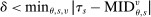 implies
  . This in turn implies

 , then
  implies
  . By the definition of
  ,
,  . Therefore, there is no applicant with
  and
and  .
.Hence, conditional on  and not being assigned a choice preferred to s, the probability of being assigned s is given by
  . Therefore, for students with
  , we have
  . Q.E.D.
Lemma 2.For all s, θ, and sufficiently small  , we have
 (19)
(19)

Proof of Lemma 2.The first line follows from Lemma 1 and the fact that  imply
imply  for sufficiently small
  .
.
For the remaining lines, note first that conditional on  , we have
  and so
  holds for small enough δ.
  therefore is the probability of not being assigned to a school preferred to s in the last three cases.
The second line then follows by the fact that  implies
  for small enough
  . The third line follows from the fact that for small enough
  ,
,

 . The last line follows directly follows from Lemma 1. Q.E.D.
Lemma 2 is used to derive Theorem 1 by characterizing  and showing that this limit coincides with
  as defined in the text.
In the first case in Lemma 2,  is constant at zero, and so
  in this case.
 for the remaining cases, note that by the differentiability of
  (recall the continuous differentiability of
  ) (Assumption 1), L'Hôpital's rule implies


 if
if  or
or  otherwise since whether
  does not depend on δ. Therefore,

 .
. if (a)
  or (b)
  for some
  . Otherwise,

 , completing the proof of Theorem 1.
A.2 Proof of Corollary 1

 . By the symmetry of conditional independence (Dawid (1979)), and because
  , this implies

 such that the first-stage effect
  . Since we assume the first-stage effect is nonzero, the conclusion follows.