Banks, Liquidity Management, and Monetary Policy
Abstract
We develop a tractable model of banks' liquidity management with an over-the-counter interbank market to study the credit channel of monetary policy. Deposits circulate randomly across banks and must be settled with reserves. We show how monetary policy affects the banking system by altering the trade-off between profiting from lending and incurring greater liquidity risk. We present two applications of the theory, one involving the connection between the implementation of monetary policy and the pass-through to lending rates, and another considering a quantitative decomposition behind the collapse in bank lending during the 2008 financial crisis. Our analysis underscores the importance of liquidity frictions and the functioning of interbank markets for the conduct of monetary policy.
1 Introduction
The transmission and implementation of monetary policy operates through the banking system. In practice, central banks set a target for the interbank market rate and implement that target via open market operations and standing facilities. The ultimate goal is to affect the amount of credit, and thus overall economic activity. It is therefore of paramount importance to understand how monetary policy affects the interbank market and, in turn, how the interbank market affects the real economy.
The leading macroeconomic framework is used for monetary policy analysis, the New Keynesian model, abstracts from the implementation and transmission of monetary policy through the interbank market. In the New Monetarist framework, interactions between money and credit are explicit, but frictions in the interbank market and its impact on bank credit have received little attention.1 Moreover, for the most part, the focus of analysis has been on a sole policy instrument, either a nominal interest rate or the nominal quantity of money. Following the 2008 financial crisis, however, disruptions in interbank markets have been met with a broad set of policy responses designed to inject liquidity into the financial system and mitigate contractions in credit. These events call for a model that can be used to analyze the effects of frictions in the interbank market and the transmission of monetary policy through the banking system.
This paper provides a tractable general equilibrium model with a banking system that articulates a notion of the credit channel of monetary policy. At the heart of the theory lies a liquidity management problem that emerges from frictions in the interbank market. Liquidity management concerns the trade-off between holding high-yield illiquid loans and low-yield liquid assets. By influencing this trade-off, monetary policy affects the supply of credit and gives rise to a credit channel. In support of this transmission channel, we document an empirical relationship between measures of disturbances in the interbank market and liquidity premia. We put this framework to work in two quantitative applications that showcase the importance of examining the transmission of monetary policy through the banking system.
In the theory, banks are competitive. Their portfolio is composed of deposits, loans, government bonds, and reserves. When a bank grants a loan and simultaneously issues deposits, it gains intermediation profits. However, deposits circulate in an unpredictable way, and thus banks face deposit withdrawal shocks. When a deposit is transferred out of a bank, another bank absorbs that liability. As occurs in practice, that transfer is settled with reserves.2 If a deposit withdrawal is too large, the bank will end short of reserves. The bank can sell bonds in exchange for reserves, but this may not be enough. At that point, the bank must incur the expense of borrowing reserves, either from the discount window at a penalty rate or from the interbank market. The interbank market is over-the-counter (OTC). The probability of finding a counterpart in the interbank market depends on the scarcity of reserves: when few banks have reserve surpluses, the interbank market rate is high, and hence a shortage is expensive. Thus, the efficiency and tightness of the interbank market affect the degree of liquidity risk. By holding a large buffer of liquid assets composed of bonds and reserves, a bank reduces its exposure to liquidity risk at the expense of intermediation profits. Tilting this trade-off, monetary policy affects the supply of bank credit by affecting liquidity premia.
From a methodological standpoint, a contribution of this paper is to integrate an OTC interbank market into a dynamic general equilibrium model of the banking system. The interbank market here is modeled after Afonso and Lagos (2015), who study the federal funds market in a repeated OTC setting and deliver predictions for the intraday volume of interbank market loans and the distribution of interbank rates. That model takes the distribution of reserve balances as a primitive. Here, the distribution of balances is endogenous, as it results from banks' portfolio management, which is in turn influenced by monetary policy. We show that, despite the nonlinear nature of the liquidity frictions, the bank's problem features aggregation, and thus the economy behaves as if there were a representative bank. The model's analytical tractability makes the analysis transparent and amenable to various applications, both theoretical and quantitative.
Analyzing the transmission of monetary policy through the banking system reveals several insights. In contrast to models in which reserve requirements exogenously determine the demand for reserves, monetary policy here affects the risk-return trade-off between holding reserves vis-à-vis loans. The central bank alters this trade-off through open market operations, both conventional and unconventional, and by setting interest rates on reserves and discount window lending. We show that, although the composition between government bonds and reserves is indeterminate for an individual bank—implying that total holdings of liquid assets are the correct measure of the precautionary liquidity demand—the composition matters at the macro level. We show that a policy that swaps bonds for reserves has aggregate effects on liquidity premia by altering the interbank market tightness. Moreover, by absorbing illiquid assets into the central bank's balance sheet, unconventional open market operations have even more potent effects. At the limit, when the interbank market shuts down entirely, only unconventional open market operations remain effective.
A central insight of the paper is that the implementation of monetary policy matters for macroeconomic outcomes. We first study how the pass-through from the interest on reserves to credit is potentially nonmonotonic and depends critically on the interaction with capital requirements. When the interest on reserves is low, deposits are in effect more costly and capital requirements do not bind. As the interest on reserves increases, banks expand deposits, reserves, and potentially credit. Once capital requirements bind, further increases in the interest on reserves necessarily contract lending. The analysis reveals that reserves can be complements to or substitutes for bank lending, depending on whether capital requirement constraints bind. We then examine how the interest on reserves and the central bank's balance sheet constitute independent policy instruments. Crucially, we show how configurations that achieve the same target for the interbank market rate generate a different lending rate and pass-through. In particular, configurations with a larger balance sheet induce a larger credit supply and a higher pass-through from the interbank market rate to the lending rate. Taken together, these findings imply that the questions on how to set a target for the policy rate and how to implement it, must be analyzed together.
A final contribution is to employ the framework to quantitatively examine the credit crunch during the U.S. financial crisis after 2008. In particular, we examine the role of aggravated liquidity conditions, as evidenced by the severe collapse in the interbank market and the increase in discount window borrowing. We devise a procedure to reverse engineer the shocks required to match the data and then feed the model with counterfactuals. Our findings suggest that disruptions to the matching efficiency of the interbank market and to the volatility of funding played a substantial role around the time of the Lehman Brothers bankruptcy. By 2010, loan demand became the dominant factor. Turning to policy, we study the contribution of conventional and unconventional open market operations to mitigating the credit crunch. We find that conventional operations had a negligible effect, while unconventional ones had a sizable impact. The quantitative analysis suggests that the move toward unconventional open market operations during the crisis was critical for the attenuation of the credit crunch.
Related Literature
Our paper relates to several branches of the literature in monetary economics, banking, and macroeconomics. One branch studies monetary policy implementation through banks' reserve management in partial equilibrium real models. Building on the seminal work of Poole (1968), several studies have analyzed recent proposed changes in monetary policy frameworks (Ennis and Weinberg (2007); Keister, Martin, and McAndrews (2008); Keister and McAndrews (2009); Ennis and Keister (2008); Martin, McAndrews, Palida, and Skeie (2013); Bech and Keister (2017)). At the center of our analysis on monetary policy, implementation is a downward sloping relation between liquidity and the interbank market rate, a feature that is common with these studies. In our model, however, it is derived in the context of an OTC interbank market, which enables us to study the interaction between monetary policy and disruptions in the interbank markets.3 Our central contribution to this literature is to examine monetary policy implementation through the lens of a dynamic general equilibrium monetary model. Analyzing interbank market rates, credit, and prices in a unified framework underscores how the choice of the target interest rate and how to implement that rate are inherently linked.
The paper also builds on the banking literature. Important examples include Diamond (1984); Diamond and Dybvig (1983); Boyd and Prescott (1986); Allen and Gale (1998); Holmstrom and Tirole (1998); and Gu, Mattesini, Monnet, and Wright (2013). For the most part, these theories have evolved separately from macroeconomics. Gertler and Karadi (2011) and Curdia and Woodford (2009) incorporated a banking sector into quantitative New Keynesian models. Following these studies, a growing literature has examined how shocks to bank equity or leverage constraints disrupt financial intermediation.4 A distinct approach is taken by Corbae and D'Erasmo (2013, 2018), who provide a model with heterogeneous banks and analyze the role of bank concentration and how it interacts with capital requirements. The present paper emphasizes interbank market frictions and the transmission of monetary policy through the liquidity premium.
The OTC nature of the interbank market builds on monetary search theory. Seminal contributions in this literature are Kiyotaki and Wright (1989) and Lagos and Wright (2005). The interbank market here is a version of the OTC model developed by Afonso and Lagos (2015).5 Related studies also include Freeman (1996) and Smith (2002), who study environments where inside money is used as a medium of exchange, as a result of spatial frictions. Williamson (2012) study an environment in which assets of different maturities have different properties as mediums of exchange. Relative to this earlier work, we have little to say about the foundations that bring about a banking architecture. Here, the focus is on the effects of trading frictions in the interbank market and the transmission of monetary policy through the credit channel.
Finally, a burgeoning literature explores other issues related to monetary policy transmission and implementation through banks' liquidity management: Piazzesi and Schneider (2018) study the link between the payments system and securities markets with a focus on asset pricing and price-level determination; Piazzesi, Rogers, and Schneider (2019) incorporates nominal rigidities; De Fiore, Hoerova, and Uhlig (2018) study the role of collateral assets for liquidity management and unconventional monetary policy; Chen, Ren, and Zha (2017) analyze the implications for shadow banking in China; Arce, Nuño, Thaler, and Thomas (2019) evaluate floors versus corridor regimes with New Keynesian ingredients; Bigio and Sannikov (2019) study the implications for individual insurance and productive efficiency; Bianchi, Bigio, and Engel (2020) provide a theory linking exchange rate fluctuations to banks' liquidity management.
Outline
The paper is organized as follows. Section 2 presents the model, and Section 3 provides theoretical results. Section 4 presents evidence on the correlation between interbank market spreads and the liquidity premium. Section 5 presents the calibration of the model and the applications. Section 6 concludes. All proofs are in the Appendix or in the Online Supplementary Material (Bianchi and Bigio (2022)).
2 The Model
We present a dynamic general equilibrium model of the banking system featuring an OTC interbank market. The presentation of the model begins with the liquidity management problem of an individual bank, followed by the description of the interbank market. We then introduce the non-financial block of the model, describing households and firms, and analyze the policies of the central bank, which we refer to as the Fed. After characterizing the problems of all agents, we define the general equilibrium and analyze the transmission of monetary policy.
2.1 Banks: Preferences and Budgets
Preferences
 are given by
 (1)
(1) is the time discount factor, and
  is the utility function over the consumption good with
  .
.Timing
Time is discrete, indexed by t, and of infinite horizon. Each period is divided into two stages: a lending (l) and a balancing (b) stage. In the lending stage, banks make portfolio decisions. In the balancing stage, banks experience random idiosyncratic withdrawals of deposits. A deposit withdrawn from one bank is transferred to another bank. That transaction must be settled with reserves. If banks lack reserves to settle that transaction, they can sell government bonds, borrow reserves from other banks or from the Fed at a penalty rate. We describe next the two stages—a summary of the timeline of events is found in Figure 11 in the Online Appendix E.
Lending Stage
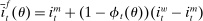
Banks enter the lending stage with a portfolio of assets/liabilities and collect/make associated interest payments. Among assets, banks hold loans,  , and liquid assets in the form of reserves,
  , or government bonds,
  . On the liability side, banks issue demand deposits,
  , discount window loans,
  , and net interbank loans,
  (which is positive if the bank has borrowed funds and negative if the bank has lent funds). All assets are nominal (denominated in units of reserves).6 Reserves are the numeraire and
  is the price level.
During the lending stage, banks choose real dividends,  , and a portfolio. The portfolio is a choice
  , which corresponds to holdings of loans, reserves, government bonds, and deposits, respectively. We use
  to denote a portfolio variable chosen in the lending stage and
  to denote the end-of-period portfolio variable in the balancing stage (and the beginning-of-period portfolio variable for
  ). Aggregate holdings are denoted in uppercase letters, for example,
  represents the aggregate loan supply.
 (2)
(2) ,
,  , and
, and  , denote the nominal returns on loans, government bonds, and deposits, respectively. The policy rates
  and
and  are interest on reserves and discount window loans set by the Fed. These rates satisfy
  ; otherwise, there is a pure arbitrage to the detriment of the Fed. The rate
  represents the fed funds rate, the average rate at which banks borrow in the interbank market, a market described below. All interest rates indexed with t are accrued between period
  and t. Finally,
  denotes taxes that are set to be proportional to bank equity.
 (3)
(3)The problem of the bank in the lending stage is to choose the portfolio and dividend payments, subject to the budget constraint (2) and the capital requirement (3).
Balancing Stage
 . At the start of the balancing stage, banks experience an idiosyncratic withdrawal shock
  . The shock generates a random inflow/withdrawal of deposits
  ; hence, the end-of-balancing-stage deposits are given by
 (4)
(4) is positive, the bank receives deposit inflows from other banks. When
  is negative, the bank loses deposits to other banks. The withdrawal shock has a cumulative distribution
  common to all banks with support
  , where
  . The distribution is continuous and satisfies
  for all t, implying that deposits are reshuffled but preserved within banks.
The randomness of ω captures the unpredictability and complexity of the payments system. The circulation of deposits is a fundamental feature of the payments system, because it enables banks to facilitate transactions between third parties: When a bank issues a loan, a borrower is credited with deposits. As the borrower makes payments to third parties, deposits are transferred to other banks. The outflow of a deposit from one bank is an inflow to another. Because the receptor bank absorbs a liability, an asset also must be transferred to settle the transaction.7 As it occurs in practice, reserve balances at the Fed are the settlement instrument.
 (5)
(5) (6)
(6) , it borrows reserves in an OTC interbank market or from the discount window. If it ends in surplus, a bank lends in the interbank market or holds reserves at the Fed. The reserves with which the bank ends the period—which must satisfy equation (5)—are therefore given by
 (7)
(7)Interbank Market
Withdrawal shocks generate a distribution of reserve surpluses and deficits across banks. When the interbank market opens, banks with a surplus want to lend, and banks with a deficit want to borrow. Because of the matching frictions, banks on either side of the market may be unable to lend/borrow all of their balances. If a bank in deficit cannot obtain enough funds in the interbank market, it must borrow the remainder from the discount window. If a bank in surplus is unable to lend all of its surplus, it deposits the balance at the Fed and earns interest on reserves. In equilibrium, because interbank rates lie between the interest rates on reserves and discount loans, banks will seek to trade in the interbank market before trading with the Fed. All loans are repaid before the next lending stage.
The interbank market is an OTC search market. We follow closely the basic formulation in Afonso and Lagos (2015) but render analytic solutions following Bianchi and Bigio (2017) that allow us to embed this friction into the dynamic model. The interbank market operates sequentially through N trading rounds. At the beginning of the trading session, each bank gives an order to a continuum of traders. If  (
( ), the bank gives an order to lend (borrow). Each trader must close an infinitesimal position, as in Atkeson, Eisfeldt, and Weill (2015). This “large family” assumption simplifies the solution of the bargaining problem by making the marginal value of the interbank loan depend only on the sign of the balance, and not on the scale. Absent this assumption, it becomes necessary to keep track of the identity of matching banks in their bargaining problems—the resulting problem of determining the distribution of matches among numerous combinations would be intractable.
The probability of a match at a given round is the outcome of a matching function that depends on the aggregate amount of surplus and deficit positions that remain open at each round. When traders meet, they bargain over the rate and split the surplus according to Nash bargaining. Key for the determination of the interbank market rate at any given round, are the rates and probabilities of finding a match in future rounds.

 denotes the aggregate surplus and
  denotes the aggregate deficit.9 If we consider a Leontief matching function with efficiency parameter λ and take the limit of N rounds to infinity (keeping the overall number of matches per balancing stage constant), we arrive at the following proposition that characterizes the split between interbank market and discount window loans,
  , as a function of θ.
Proposition 1.Given θ, the amount of interbank market loans and discount window loans for a bank with surplus  is
is
 (8)
(8) . Analytic expressions for
  are presented in Appendix A.
Banks short of reserves patch a fraction  of their deficit in the interbank market and the fraction
  in the discount window. Similarly, a bank with surplus lends a fraction
  in the interbank market and keeps the remaining balance,
  , at the Fed. These fractions are endogenous objects that depend on market tightness. If many banks are in deficit (surplus), the probability that a deficit bank finds a match is low (high). Market clearing in the interbank market requires
  . We say that the interbank market is active if
  and inactive otherwise.
Proposition 1 also characterizes the mean interbank market rate,  , as a function of the market tightness. The Fed funds rate is a weighted average of the corridor rates
  and
and  . The weight, given by
  , is an endogenous bargaining power, as in Afonso and Lagos (2015). If many banks are in deficit, the Fed funds rate is closer to
  because this lowers the outside option and the bargaining power of banks in deficit. Conversely, the Fed funds rate is closer to
  if more banks are in surplus.10
As shown in Appendix A, the functional forms for  and
and  depend on two structural parameters: the matching efficiency, λ, and the bargaining power, η. In particular, for given θ, a higher efficiency leads to higher fractions of matches
  , and a higher η increases the effective bargaining power of banks in deficit, lowering the Fed funds rate.
A single function, which we call liquidity yield function, encodes the payoffs from having surplus or deficit of reserves and reflects the activity in the interbank market.
Definition 2.The liquidity yield function is
 (9)
(9) , the bank earns an average yield
  per unit of surplus and when
  , the bank pays an average yield
  per unit of deficit. The fact that
  creates a kink in χ and generates a positive wedge between the marginal cost of reserve deficits and the marginal benefit of surpluses.11
The liquidity yield function will be used below to characterize the dynamic bank problem. We use  to denote the real liquidity yield function in terms of the portfolio where
  is the gross inflation rate. We also define
  to be the gross returns on asset
  .
.
Discussion of Model Features
Some model features that merit discussion are designed to capture institutional features of the banking system. A first feature is that banks are endowed with risk-averse preferences. These preferences are necessary to generate slow-moving bank equity, as observed in practice, and can be rationalized by costs of equity issuances.
A second feature has to do with the nature of settlements in the balancing stage. When banks receive deposit outflows, they must settle with the bank absorbing the deposits using reserves. This feature is in line with actual institution arrangement and can be microfounded by appealing to informational frictions (Cavalcanti, Erosa, and Temzelides; Lester, Postlewaite, and Wright (2012)). Upon facing withdrawal shocks, banks can trade government bonds in exchange for reserves, but loans are illiquid. The lack of a liquid market for loans can be explained by a moral hazard problem. On the other hand, the assumption of a Walrasian exchange for government bonds is for simplicity, but it captures that this is a deep market that operates with relatively fewer frictions.12 In addition, the interbank market is modeled as an OTC market. This feature is the empirically relevant one, as established by Ashcraft and Duffie (2007), and in line with the bilateral and unsecured nature of this market.
Finally, we note that positive reserve requirements, are not essential for the theory. What is key for the emergence of liquidity premia is that there is a lower bound on reserve holdings.13
2.2 Nonfinancial Sector
The nonfinancial block is presented in detail in the Online Appendix F. This block is composed of households that supply labor and save in deposits, currency, and government bonds. Firms produce the final consumption good using labor and are subject to a working capital constraints. This block delivers endogenous demand schedules for working capital loans, and household's deposits, government bonds, and currency. These household schedules emerge from asset-in-advance constraints, as in Lucas and Stokey (1983). We purposefully work with quasi-linear preferences, as in Lagos and Wright (2005), so that these schedules are not forward-looking. The schedules for the asset-demand system of the non-financial block are summarized in the proposition below.
Proposition 3.Given the nonfinancial sector block presented in Appendix F, we have that: (i) The firm loan demand is  and output is
  with
with  ;
;
(ii) The household deposits, currency, and government bond demand schedules have the form

 for all
  and where
  is the corresponding rate of return to the household.
The household schedules are iso-elastic as long as returns are lower than the inverse of household discount factor  .14 The parameters
  and
and  are, respectively, elasticity and scale coefficients, which depend on structural parameters regarding technology and household preferences; see Table 4 in Appendix F for the conversion from the structural to the reduced form parameters in these schedules. The parameter
  represent an asset satiation point.
A convenient property is that once we solve for the equilibrium real rates—by equating the asset supply and demand schedules derived from banks and the reduced form schedules obtained from the nonfinancial sector—we can obtain output, employment, and household consumption. For the rest of the paper, we do not make further references to the nonfinancial block and work directly with the iso-elastic portion of these schedules—there always exists a  that guarantees that this is the case.
2.3 Monetary and Fiscal Authority
The Fed's policy tools are the discount window rate, the interest on reserves and open market operations (OMO), both conventional and unconventional. On the asset side, the Fed holds discount window loans,  , private loans,
  , and government bonds,
  . Government bonds are issued by the fiscal authority, which we denote by
  . The supply of Fed liabilities
  can be held as currency by households or as bank reserves (i.e.,
  ).
).
 (10)
(10) , and taxes on banks, T, to balance the budget constraint.
 (11)
(11) are set as a residual, in the spirit of passive fiscal policy.15
2.4 Competitive Equilibrium
The competitive equilibrium is defined as follows.16
Definition 4.Given an initial distribution  and a deterministic sequence of government policies
  , a competitive equilibrium is a deterministic path for aggregates
  , a stochastic sequence of bank policies
  , a deterministic sequence of interest rates
  , a deterministic sequence for the price level
  , and a deterministic sequence of matching probabilities
  , such that
- (i) bank policies solve the banks' optimization problems, and
 are given by Proposition 1;
 - (ii) the government's budget constraint (10) is satisfied and the tax on banks follow (11);
- (iii) households and firms are on their supply/demand schedules, as given by Proposition 3;
- (iv) markets for deposits, loans, reserves, and government bonds clear;
- (v) the matching probabilities
 and the Fed funds rate
  are consistent with the market tightness,
  , induced by the aggregate surplus and deficit
  and
and  , as given by Proposition 1.
We refer to a stationary equilibrium as a competitive equilibrium in which all real aggregates are constant and the value of all nominal variables grow at a constant rate. A steady-state equilibrium is a stationary competitive equilibrium in which the price level is constant.
3 Theoretical Analysis
We first examine the bank's portfolio problem and show that it can be reduced to only two choices, one about leverage and the other one about liquidity. We then provide an aggregation result by which aggregate equity is the only state variable. Finally, we examine the liquidity premia and the monetary policy transmission.
3.1 Recursive Bank Problems
Denote by  and
and  the bank value functions during the lending and balancing stages, respectively. To keep track of aggregate states, which follow a deterministic path, we index the policy and value functions by t. To ease notation, we omit the individual superscript j and suppress the time subscripts inside the Bellman equations.
At the beginning of each lending stage, the individual states are  . Recall that choices in the lending stage are consumption, c, and portfolio variables
  . These portfolio variables together with the idiosyncratic shock, ω, become the initial states in the balancing stage. The continuation value is the expected value of the balancing stage
  under the probability distribution of ω.
We have the following bank problem in the lending stage.
Problem 5. (Lending-Stage Bank Problem)
 (12)
(12)
In turn, the balancing-stage problem is the following.
Problem 6. (Balancing-Stage Bank Problem)
 (13)
(13) (Evolution of loans)
 (Evolution of deposits)
 (Evolution of reserves)
 (Reserve surplus)
 (Interbank market)
 , banks in deficit choose to sell all government bonds. In equilibrium, as long as the amount of government bonds held by banks in deficit does not exceed the surplus of reserves, we have that
  and banks in surplus are indifferent between selling their reserve surplus for bonds. We assume this case holds for the rest of the paper.17
 (14)
(14) ). The following proposition presents the characterization.
Proposition 7. (Homogeneity and Portfolio Separation)The bank's problem has the following features:
- (i) Problems 5 and 6 can be combined into a single Bellman equation with equity as the only individual state variable, and the holdings of government bonds and reserves can be consolidated into a single liquid asset
 ,
,
 (15)
(15)
- (ii) The optimal portfolio in (15) is given by the solution to
 (16)
(16) - (iii) The optimal bank dividend–equity ratio
 is
and
is
and (17)
(17) .
. - (iv) Portfolios scale with equity. We have that
 from (15) can be recovered from the optimal portfolio weights
  obtained in (16) via the relationship
  . The individual holdings of reserves and government bonds satisfy
 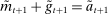 .
.
There are four items in Proposition 7. Item (i) shows that we can synthesize the value functions in (12) and (13) into a single Bellman equation with real equity as a single state variable. The liquidity yield function, χ, shows up in this Bellman equation summarizing parsimoniously the liquidity frictions. Equation (15) is, in effect, a portfolio savings problem. The bank starts with equity, e, can lever by issuing deposits  , pays dividends, and makes portfolio investments. The choice of assets can be split into loans,
  , and liquid assets, ã—the composition of liquid assets between reserves and government bonds is indeterminate. The continuation value of the bank depends on next period equity
  , which in turn depends on the realized portfolio return. The proposition establishes that, although there is a distribution of bank equity, all banks are replicas of a representative bank: item (ii) indicates that banks choose the same portfolio weights; item (iii) shows that all banks feature the same dividend rate; and item (iv) shows that banks' portfolio investments are linear in equity.
A key takeaway of the proposition is that the model aggregates. While aggregation is known to hold under linear budget constraints and homothetic preferences, a contribution here is to show that aggregation also holds despite a kink in the return function. This showcases how to integrate search frictions into a standard dynamic model with a representative agent.
 (18)
(18) . This equation says that next-period aggregate equity is given by the current aggregate equity net of dividend payments times the aggregate portfolio return. Implicit in (18) is that (i) the returns on interbank market loans cancel out on aggregate; (ii) Fed profits and the interest earned on government bonds by banks are compensated with taxes.
Another takeaway from Proposition 7 is that at the individual level, the composition between reserves and government bonds is indeterminate. Key to this result is that there is a Walrasian market between reserves and government bonds that allows banks to freely reverse any portfolio mix between reserves and government bonds once they face a withdrawal shock. This is different for loans, which stay with the bank and, therefore, the portfolio mix matters.
 (19)
(19) (20)
(20) from the market-clearing condition for government bonds,
 (21)
(21) to obtain the demand for reserves. Equation (20) then shows that for a given weight on liquid assets ā, the market tightness increases with a higher value of
  . The important lesson is that, even though reserves and government bonds are perfect substitutes at the individual bank level, the composition of liquid assets matters at a macroeconomic level.
Discussion on Aggregation Property
Thanks to this aggregation property, the model provides a sharp characterization of the bank liquidity management problem and renders a transparent analysis of monetary policy transmission. Moreover, from a computational point of view, a notable advantage is that the model is straightforward to compute, as aggregate equity is the single state variable. On the other hand, a limitation is that the model cannot speak to features such as heterogeneous responses to monetary policy, size-dependent policies, or shocks that give rise to changes in concentration, which emerge in models with an endogenous size distribution (see Corbae and D'Erasmo (2018)).
3.2 Liquidity Premia
 , total liquid assets ā, and deposits
  to maximize the certainty equivalent of the bank's return on equity:

Proposition 8. (Liquidity Premia)Let  be a solution to the portfolio problem in Proposition 7. Then we have the following equilibrium liquidity premia (LP) on loans, government bonds, and deposits:
 (Loan LP)
 (Gov. Bond LP)
 (Deposit LP)
 is the Lagrange multiplier on the leverage constraint and
  . Furthermore,
  . The last two inequalities become equalities if
  .
.
Proposition 8 displays the LP of each asset relative to reserves.18 Consider first Loan LP. Loans command a higher direct return than reserves because reserves also yield a return in the interbank market. The premium is a risk-adjusted interbank market return: if the bank ends in surplus, a marginal reserve is lent out at an average of  while if the bank ends in deficit, the marginal reserve has an additional value of
  . We say that banks are satiated if the premium is zero.
The Gov. Bond LP is also positive but lower than the premium on loans.19 In a deficit state, a bank that holds a government bond sells it and saves the spread  . The bank therefore obtains
  the next period, which is the same as the return of reserves in a deficit state. To guarantee positive reserve and government bond holdings, we must have that the return on a surplus state must also be equalized. Because reserves yield
  in a surplus state, we have that the return on bonds must satisfy
  . This positive premium reflects how payments clear with reserves but not with government bonds.20
Finally, Deposit LP can be of either sign. The deposit LP has three terms: The first term captures the expected change in the surplus, considering the reserve requirement—the effect is proportional to the LP of loans because withdrawals are mean zero, and is therefore positive. The second term is a liquidity-risk premium, which captures that an increase in deposits raises liquidity risk. The risk premium is present even if banks are risk neutral because the concavity in χ produces endogenous risk-aversion.
Role of OTC Frictions
The analysis of liquidity premia clarifies the fundamental role of OTC frictions for the transmission of monetary policy. As we take the efficiency parameter  , we recover a Walrasian interbank market.21 In a Walrasian market, if the banking system has an overall excess of reserves, we have
  , while if the banking system has an overall deficit of reserves, we have
  . Meanwhile, if aggregate excess reserves are exactly zero, the Fed funds rate is indeterminate. This implies that the costs of deficits equals the benefits of a surplus,
  and changes in withdrawal risks would have no effects. In addition, OMO would be neutral unless aggregate excess reserves change sign, for example, in a Walrasian market with
  , there no effects of OMO because aggregate excess reserves are always positive in this case.
Figure 1 presents  ,
,  and the Fed funds rate as a function of the log inverse of market tightness θ, for the frictional OTC market (left panel) and the Walrasian market (right panel). In the case of the OTC market, we can see how as liquidity increases and we move along the x-axis, the Fed funds rate falls closer to the floor of the corridor. The figure illustrates how depending on the target for the interbank market rate, the central bank can adjust the amount of liquidity to aim at a desired target.

OTC versus Walrasian markets.
The classic Poole model also generates a smooth downward curve for the interbank market rate as a function of the real supply of government liquidity, as in Figure 1(a). However, it does so by assuming that the interbank market, modeled as a Walrasian market, closes before withdrawal shocks are realized. Like Afonso and Lagos (2015), our model can thus be seen as a microfoundation of such a downward-sloping relationship.22 Notably, the model predicts that withdrawal risk can have very different implications depending on the interbank market's functioning. Another notable difference is that the Poole framework is, in effect, a partial equilibrium model and, therefore, does not allow for a joint analysis of prices, credit, and macroeconomic aggregates. When we present the model's applications in the next section, we will show how embedding this OTC interbank market in a general equilibrium model gives rise to novel policy implications regarding monetary policy transmission. Namely, we will show that whether the central bank hits the target by shifting the balance sheet or by changing corridor rates has macroeconomic effects.
3.3 Policy Analysis
This section analyzes the effects of monetary policy. The main insight is that Fed policies can alter the liquidity premium and induce real effects, a formalization of the credit channel. Let us first discuss the price-level determination.
Price-Level Determination
 (22)
(22) , and a set of real rates, the portfolio demand for total real liquid assets is determined. The price level must be such that, at equilibrium real rates, the real supply of liquid assets equals the real liquidity demand. Once we substitute the clearing condition for government bonds, (21) and use
  , we obtain a quantity equation but now expressed in a more familiar way, in terms of monetary balances:
 (23)
(23)We note that the price level remains determined, even if banks are satiated with reserves. In this regard, our paper relates to Ennis (2018), who analyzes the link between money and prices in a perfect-foresight model with a static banking system. He shows that when capital requirements are slack, a policy of paying interest on reserves equal to the market return of the risk-free asset leads to an indeterminacy result, but when the capital requirement constraint binds, the real demand for reserves is determined, and hence the price level. One difference in our setup is that the presence of equity constraints in our framework implies that the price level is determined even absent binding capital requirements. In addition, here, the price level is determined through a quantity theory equation involving both government bonds and reserves.
Classical Monetary Properties
The model features classic long-run neutrality: an increase in the scale of  leads to a proportional increase in the price level without any changes in real allocations. On the other hand, changes in the permanent growth rate of the Fed's balance sheet do have real effects, unless all nominal policy rates are adjusted by inflation to keep real rates constant—and when the demand for real currency balances is perfectly inelastic. Both results are proven in the Online Appendix F.
OMO
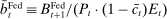
Policies that produce real effects operate through the liquidity premium. We define conventional (unconventional) OMO as a swap between reserves and government bonds (loans). The next proposition characterizes the effects of an OMO by which the Fed exchanges reserves for loans and government bonds in the initial period and reverses the operation the following period.
Proposition 9. (Real Effects of OMO)Consider an original policy sequence with a Fed balance sheet  and an OMO at
  reversed at
  . That is, consider an alternative policy sequence that differs from the original one only in that
  ,
,  , and
, and  , for
, for  and
and  and
and  . We have the following two cases:
(i) Functioning interbank market: If  , then the OMO has effects on prices and aggregate asset allocations if and only if banks are not satiated with reserves at
  under the original allocation.
(ii) Interbank market shutdown: If  , and the operation is conventional (
 ) the OMO induces the same sequence of prices and real asset allocations; If the operation is unconventional (
 ), then the OMO has effects on prices and aggregate asset allocations if and only if banks are not satiated with reserves at
  under the original allocation.
The proposition establishes that, when banks are satiated with reserves, open market operations are irrelevant, as in Wallace (1981). In effect, when banks are satiated, all assets are perfect substitutes. As a result, for every unit of loans (government bonds) that the Fed purchases, banks reduce loan holdings (government bonds) by one unit and increase reserves by the same amount.24 In effect, there are no changes in the real returns. Moreover, there are no changes in the price level.25 Away from satiation, however, the operations alter the liquidity premium and induce a change in the total amount of loans. When the Fed swaps government bonds or loans for reserves, this increases the relative abundance of reserves and reduces the costs from being short of reserves for an individual bank. As a result, for a given level of bank equity, this contributes to reduce the liquidity premium. Ultimately, this increases the supply of bank lending.
Moreover, the swap of government bonds or loans for reserves leads to an increase in the price level, but not one-for-one. Notice that for a given price level, a conventional OMO keeps constant the total amount of liquid assets. At the same time, since the composition is tilted toward reserves, market tightness θ falls (see equation (20)), leading to a lower demand for total liquid assets. It then follows from (22) that the price level increases but less than proportional to the increase in  .
.
Finally, an important result is that standard operations are irrelevant if the interbank market is shut down ( ). When the interbank market is shut down, the benefits of holding liquid assets are independent of the abundance of reserves on the aggregate because reserves cannot be lent to other banks. In particular, we have
  ,
,  . As a result, a swap of reserves for government bonds simply changes the composition of liquid assets without any real effects. This result shows that, in an extreme event of an interbank market shutdown, the Fed should conduct unconventional OMO if it aims to reduce the liquidity premium and stimulate credit.
Bounds on the Lending Rate and the Friedman Rule
This section describes the set of rates that can be induced by the Fed in a stationary equilibrium and connects with a banking version of the Friedman rule. We refer to the Friedman rule as a monetary policy where the Fed lends at the discount window without penalty, that is, when the discount window rate equals the rate on reserves.
Definition 10. (Friedman Rule)Monetary policy is consistent with a Friedman rule if  .
.
Under this rule,  . Hence, banks are satiated, not through large holdings of liquid assets but through free borrowing from the discount window.26 As a result, there are no liquidity premia. This rule is in the same vein as the common version of the Friedman rule, under which the nominal interest rate on government bonds is zero, and there is no opportunity cost of holding currency. Likewise, in this banking version, there is no cost of being short of reserves. Moreover, with strictly positive liquid assets, there is also no opportunity cost of holding reserves, since
  .
.
Notice that, as defined here, there are many values of  consistent with this Friedman rule, and as we will show, there is a different loan rate associated with each value of
  .27 We denote by
  the stationary loan rate that prevails if the monetary authority follows a Friedman rule associated with a fixed stationary interest on reserves
  . The following proposition characterizes this stationary loan rate, focusing on the case with
  and
and  .
.
Proposition 11. (Stationary Loan Rate Under Friedman Rule)Assume that  and
and  . Consider the following parameter condition:
 (24)
(24) be the unique solution to


Slack Capital Requirements: If (24) holds, then capital requirements are slack and
 (25)
(25) , then
  (with
(with  binding strictly if
  ). In all cases, the deposit rate equals
  .
.Binding Capital Requirements: If (24) does not hold, capital requirements are binding and
 (26)
(26) . Moreover, if
  , then
  (with
(with  strictly binding if
  ).
).To characterize the stationary lending rate, Proposition 11 exploits the fact that in any stationary equilibrium, the return on bank equity equals  . There are two cases to consider depending on whether capital requirements bind, as determined by (24). Consider first the case of slack capital requirements. In this case, we know that the deposit rate must equal the loan rate. We also have that if
  , banks are at a corner of liquid assets and
  . Instead, if
  , banks hold liquid assets in equilibrium, in which case
  . Notice that because in general equilibrium the after-tax return of liquid assets is zero, a loan rate
  guarantees stationarity. When the capital requirement constraint binds, the characterization is similar except that there is a spread between the loan rate and the deposit rate. As a result, we have that
  becomes equal to
  for lower values of
  compared to the case with slack capital requirements.28
Observe that  can be raised to any arbitrary level simply by raising
  . Intuitively, there is no upper bound on the lending rate because the Fed has the ability to crowd out loans by paying a higher interest rate on reserves (financed with bank taxes). On the flip side, by lowering the rate on reserves, the Fed lowers the lending rate, but only to the point where reserves are no longer held in equilibrium. Once banks are at a corner with zero reserves, further declines in
  have no effects.
Proposition 11 applies to stationary equilibria induced by the Friedman rule. Next, we discuss how the characterization of  allows us to obtain bounds on the lending rate that can be induced by policies away from the Friedman rule.
Corollary 12.Consider any stationary policy sequence such that  and
and  and let
  . Then the stationary lending rate satisfies
  .
.
The corollary says that, if we consider any policy such that 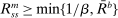 , then the lending rate induced by the Friedman rule constitutes a lower bound. The qualification
  is important, as it ensures that banks hold positive liquid assets in equilibrium. The idea is that considering equilibrium with strictly positive liquid assets, a policy that raises the liquidity premium necessarily raises the lending rate above the one that would prevail under the Friedman rule.29
The Friedman rule is not only useful for understanding the set of rates that can be induced by policies but also for characterizing efficiency. The following proposition establishes the Friedman rule is sufficient to achieve efficiency when capital requirements do not bind.30
Proposition 13.Assume that (24) holds, and that households have the same discount factor as banks  . Then the stationary equilibrium is efficient if the Fed follows a Friedman rule policy where
  .
.
Discussion on Normative Issues
The results here regard positive analysis. Having established that a version of the Friedman rule achieves efficiency, it is important to discuss what frictions outside the model could motivate a deviation from the Friedman rule. First, because of macroprudential concerns, the Fed may want to reduce the amount of bank credit and use monetary policy for such an objective, as advocated by Stein (2012). Another concern relates to the costs of eliminating liquidity premia. For example, eliminating the LP may require the Fed to hold a large balance sheet, exposing it to credit risk or interest-rate risk, features outside of this model. Finally, there is a moral hazard consideration when lending reserves freely (see Cavalcanti, Erosa, and Temzelides (1999), Hoerova and Monnet (2016)). We leave for future work the assessment of the tradeoffs that emerge in the face of these considerations. However, we believe our model provides a useful setup to study these normative aspects. Section 5.2 shows indeed how the Fed can use different instruments to balance multiple policy objectives.
4 Empirical Evidence
Over the last decade, a large empirical literature has developed conveying evidence that liquidity frictions play an important role in financial markets. The goal of this section is twofold. First, we provide new evidence that specifically point toward the importance of the interbank market. Second, we discuss other available empirical evidence that supports our key mechanism.
A central prediction of the theory is that frictions in the interbank markets are translated, at the macro level, into a premium for liquid assets. To examine whether this relationship is present in the data, one needs measures both of the frictions in the interbank market and asset liquidity premia.
Regarding the measure of liquidity premia, we use two measures constructed in Nagel (2016): the spreads between the generalized collateral repo rate (GC) and the certificate deposit (CD) with respect to the 3 month T-bill rate.31 It is worth noting that the liquidity premium is large, reaching 4% around 2008, indicating that banks are willing to forgo large returns to hold assets that can be easily sold.
Regarding the measurement of interbank market frictions, the relevant variable in our model is the spread  . To the extent that the matching probabilities are not observable, the spread is also unobserved. As a proxy, we use the dispersion in interbank market rates, also proposed in recent work by Altavilla, Carboni, Lenza, and Uhlig (2019).32 Indeed, our model predicts that high withdrawal risk and matching efficiency in the interbank market produce greater dispersion in interbank rates. More precisely, we first use the daily distribution of the Fed fund rates provided by the New York Fed and compute the daily spread between the maximum and the minimum interbank market rates observed.33 We then construct a monthly time series by averaging the daily observations. We denote this variable as FF range.
Equipped with these measures, we proceed to test the relationship between the two variables. To be clear, our goal is not to establish causality but to argue that these variables are positively correlated, as suggested by the model. Panels (a) and (b) of Figure 2 present the scatter points of the GC and CD against the FF range series, respectively, and panel (c) presents the monthly series for the GC and CD spreads and the FF range, from June 2000 and December 2011. Table I reports results from an ordinary least squares regression. The positive correlation between the FF range and the two measures of liquidity premia is striking. Columns (1) and (4) present the results for the baseline univariate regressions. Columns (2) and (5) show that the sign of the regression coefficients are unchanged after the average Fed funds rate is included, an indication that dispersion in rates captures information not contained in the policy target. Similarly, the correlation remains even when we include the VIX index, which suggests that dispersion in rates is picking up uncertainty inherent to the interbank market. The standard deviation of FF range series is 60bps, so the average impact on liquidity premia are 16bps and 36bps on the GC and CD spreads, respectively. This average impact may seem small. However, the FF range series is highly skewed (Hamilton (1996)). The FF Range series is above 200bps in 5% of the sample, and these events produce an impact of 50bps and 120bps on the GC and CD spreads, respectively. Online Appendix L presents additional robustness exercises.

Liquidity premia and Fed funds range. Note this one: Each point in the scatter plots in panels (a) and (b) represent a monthly observation. Panel (c) presents the associated time series. Online Appendix K.1 provides details of the data series.
|
(1) |
(2) |
(3) |
(4) |
(5) |
(6) |
|
|---|---|---|---|---|---|---|
|
GC Spread |
GC Spread |
GC Spread |
CD Spread |
CD Spread |
CD Spread |
|
|
FF Range |
0.208 |
0.175 |
0.159 |
0.672 |
0.721 |
0.587 |
|
(12.57) |
(11.08) |
(9.75) |
(10.17) |
(10.32) |
(8.95) |
|
|
FF Rate |
0.0291 |
0.0374 |
−0.0428 |
0.0232 |
||
|
(5.95) |
(6.87) |
(−1.98) |
(1.06) |
|||
|
VIX |
0.0857 |
0.687 |
||||
|
(3.10) |
(6.17) |
|||||
|
Constant |
0.0395 |
−0.00523 |
−0.272 |
0.0330 |
0.0988 |
−2.038 |
|
(2.53) |
(−0.33) |
(−3.11) |
(0.53) |
(1.41) |
(−5.79) |
|
|
Observations |
138 |
138 |
138 |
138 |
138 |
138 |
- Note: t statistics in parentheses.
These results on the importance of interbank market frictions should not come as a surprise in light of other available evidence.34 The scale of the interbank market is large: banks in the United States clear about 3.3 trillion USD transactions daily. At a narrative level, the August 2019 Senior Financial Officer Survey reports that the primary reason why banks currently hold reserves is to meet deposit outflows. In fact, 72% of the respondents regard as very important holding reserves to meet deposit outflows (compared with 10% who regard as very important to earn the interest on reserves).35 In the next section, we calibrate our model and show how interbank market frictions matter for the monetary transmission.
5 Applications
We now provide two applications of our model to address key questions at the intersection of monetary policy and banking. We use a version of the model calibrated to the United States banking system, as we explain next.
5.1 Calibration
We calibrate the steady state of the model using data from 2006 as a reference period. In Section 5.3, we then extend the calibration analysis to the crisis and post-crisis period. Online Appendix K.1 provides the details of data measurements and sources.
Model Period
We define the time period to be a month and use annualized rates to describe the calibration. The choice of a month is guided by several factors. On the one hand, the Federal funds market operates daily, and reserve requirements have been traditionally computed based on a two-week window average over end-of-day balances. On the other hand, bank portfolio decisions and loan sales typically take longer than two weeks to materialize.36 In addition, shocks and overall positions in the interbank market are likely to be persistent, whereas they are not in the model. Capturing these institutional details would require a more complex model with multiple balancing stages and additional state variables to keep track of lagged reserve requirements. We view a monthly model as a parsimonious compromise between the daily nature of the Federal funds market, the bi-weekly nature of regulation, and the lower frequency of bank portfolio adjustments. The choice of a monthly model is also practical. Once we turn to the application in Section 5.3, most data are available monthly.
Additional Features
We extend the environment with two additional features to enrich the quantitative applications. These features only modify the portfolio problem (16) without altering any other condition in the model. First, we allow for Epstein–Zin preferences. Assuming a unit intertemporal elasticity of substitution (IES), this implies that the dividend rate simplifies to  . Second, we introduce credit risk. In particular, we assume that the return of loans is given by
  , where δ follows a log-normal distribution with standard deviation
  and zero mean. The shock δ is distributed identically across banks and is independent of ω. By the law of large numbers, the average return across banks is
  ; hence the law of motion for aggregate equity remains the same. We introduce this second feature because it allows us to devise a procedure to match key moments in the data and to provide an exact decomposition of the decline in credit in Section 5.3. The volatility that we need to replicate the asset portfolio is small. In scale, it is about 6% of the liquidity premium.
Distribution of Withdrawal Shocks
For the distribution of withdrawal shocks, Φ, we assume that  is distributed log-normal with standard deviation
  and zero mean. A log-normal distribution approximates well the empirical distribution of excess reserves.
External Calibration
We set  externally. We list their values in Table II. We set the risk aversion to 10, a standard calibration of Epstein–Zin preferences used in asset pricing models (e.g., Bansal and Yaron (2004)). With a unit IES, stationarity of aggregate bank equity implies
  . Given the targeted portfolios and returns explained below, we obtain a discount factor
  .37
.37
|
Value |
Reference |
|
|---|---|---|
|
External Parameters |
||
|
Discount factor |
β = 0.981 |
Stationarity |
|
Risk aversion |
γ = 10 |
|
|
Interest on reserves |
im = 0 |
Observed |
|
Discount window rate |
iw = 11% |
Measured Stigma |
|
Steady-state inflation |
π = 2% |
Inflation Target |
|
Fed holdings of loans |
BFED = 0 |
Observed |
|
Government bonds |
GFA − GFed = 0.489 |
Observed |
|
Reserve requirement |
ρ = 0 |
Observed |
|
Elasticities |
ϵb = −ϵd = −ϵg = −35 |
Literature |
|
Deduced Parameters |
||
|
Matching friction |
λ = 7.9 |
W/(W + F)=0.035% |
|
Volatility of withdrawals |
σω = 0.12 |
W/(D + E)=0.0011% |
|
Bargaining powers |
η = 0.15 |
|
|
Credit Risk |
σδ = 6% × LP |
|
|
Capital requirement |
κ = 8.8 |
Bank Leverage |
|
Loan demand intercept |
Θb = 10.9 |
Loan LP = 50bps |
|
Deposit supply intercept |
Θd = 9.4 |
Rd = 2% |
|
Bond demand intercept |
Θg = 0.275 |
Gh/G = 0.56 |

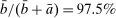
Regarding regulatory policies, we set  . While regulatory reserve requirements were about 10% in the reference period, the use of sweep accounts has implied that the most relevant constraint is that reserves cannot go negative. For that reason, we calibrate the effective requirement to zero.38
In line with the pre-crisis landscape,  and
and  are set to zero as baseline values, but we then vary these values as we analyze policies. The relevant value for the discount window rate incorporates the well-documented stigma associated with discount loans. We deduce the stigma by considering the difference between the highest interbank market rate observed and the statutory discount window rate. This approach is reasonable because the fact that many banks borrow at interbank rates above the discount rate implies there are nonpecuniary costs associated with the discount window. Accordingly, we construct a time series for the maximum observed interbank market rate and average out the differences with respect to the statutory discount window rates. The procedure yields a stigma of 5% amounting to a de facto discount window rate of 11%.39
We set the consolidated government bonds to be consistent with the holdings of government bonds by banks and households. In particular, based on Call Report data, we have that holdings of government bonds represent about 10% of banks' assets, whereas households hold about  of total holdings (Krishnamurthy and Vissing-Jørgensen (2012)). Using these two observations, we obtain
  . Normalizing the real steady-state equity to one and using the target leverage ratio discussed below, we obtain a value of 0.489. The growth rate of money balances is set to be consistent with a steady-state annual inflation of 2% per year.
Finally, we set loan demand elasticity with respect to the annualized loan rate to 2.5, which is in the range of empirical studies (see, e.g., Gilchrist, Yankov, and Zakrajsek (2009)), and use the same value for the elasticity of the supply of deposits and the household's government bonds demand.40 Neither elasticities matter for the stationary equilibrium, they only matter for transitional dynamics.
Deduced Parameters
The remaining set of parameters is  . This set is obtained by targeting a set of moments from the data. The data that we employ are the size of interbank loans relative to deposits
  ; the discount window loans relative to deposits
  ; an average Federal funds rate
  ; a measure of the loans liquidity premium LP; and portfolio holdings for loans, government bonds, and reserves
  ; and a deposit rate
  . Our procedure allows us to sequentially determine each of these parameters.
A summary of the procedure to obtain these parameters is as follows; details are relegated to Online Appendix K.3. We use  to refer to parameter or variable x deduced from the equilibrium conditions. If a variable enters without that symbol, it is measured directly from the data.
 , deduced from observed activity in the interbank market relative to discount window loans. We first infer the probability that a reserve deficit position is matched in the interbank market, using
  . When the model's implied market tightness is
  , we obtain

 . The condition
  is verified in a later step.
 from the definition (19). Then we use
  to deduce
  as the implicit solution to

 using
using

 defined in Appendix A and a measurement of the market tightness
  consistent with the previous steps.41
The fourth step is to obtain a value for credit risk,  , which we infer by rationalizing the bank portfolios given the returns of assets and liabilities, and the liquidity yield function χ. Given all the objects we have so far, we can compute directly
  and
and  .42 The return on loans is deduced using the equilibrium condition
  , where LP is observed in the data as constructed by Del Negro, Eggertsson, Ferrero, and Kiyotaki (2017).
 , and a leverage requirement κ, such that the bank optimization problem delivers the observed portfolios in the data

 is over δ and ω.43
Finally, given total credit supply in the model, the value for  is chosen to guarantee that
  is the equilibrium return using
  . We proceed analogously for
  using the target for the deposit rate and the amount of deposits, and for
  using the amount of government bonds owned by households and the equilibrium rate on government bonds.
5.2 Implementation of Monetary Policy and Pass-Through
In the first application, we examine the implementation of monetary policy and the pass-through from policy rates to lending rates. We address the following questions: What are the effects of varying the interest on reserves (IOR) on bank credit? What are the different policy configurations that can implement a target for the Federal funds rate? What are the implications of these different configurations for the lending rate and pass-through of interest rates?
IOR and Capital Requirements
We first examine the effects of changes in the IOR. In the United States, interest on reserves was introduced in October 2008. Since then, it has generated many policy discussions along different fronts, specifically on whether it contracts or expands bank lending.44 The following analysis shows that the effects on bank lending may be nonmonotonic. In particular, whether credit increases or decreases with the IOR depends on whether capital requirements bind.
We study how the stationary equilibrium changes as we vary the steady-state IOR, while keeping all other policies and model parameters constant. Figure 3 presents the results.45 In panel (a), we display the steady-state lending rate as a function of the IOR. The figure shows a nonmonotone pass-through. For low IOR, increases in the IOR lead to a slight decline in the lending rate and stimulate credit. For high IOR, increases in the IOR lead to a sharp increase in the lending rate and depress credit. In panel (b), we also display the portfolio weights as we change the IOR. As the figure shows, the change in the sign of the pass-through from the IOR to the lending rate occurs at exactly the point in which the deposit portfolio share becomes constant and the capital requirement begins to bind.

Stationary equilibrium lending rate and portfolios as a function of IOR. Note: The vertical dashed line denotes the value of the IOR at which point the capital requirement binds. We use the benchmark calibration, except that we set κ = 31, implying that the capital requirement holds with equality but it does not bind for im = 0. We also use a perfectly elastic supply of deposits to mute the effects on the interest rate on deposits.
 be the bank's risk-adjusted expectation, this premium can be written as
 (27)
(27) has a direct one-for-one effect on
  , given portfolio weights
  . Notice also that capital requirements bind when the IOR is high. This is because in effect, a high IOR makes it less costly to issue deposits. When capital requirements bind,
  and leverage is therefore invariant to the IOR, but ā increases with
  . The increase in the liquidity ratio lowers the liquidity premium but only partially offsets the direct effect of the increase in
  . This means that when capital requirements bind, reserves and loans are substitutes and an increase in the IOR is necessarily contractionary.
When the IOR is low, by contrast, capital requirements are nonbinding. Capital requirements do not bind for low IOR because a low IOR increases the costs of insuring against deposit withdrawals, hence making deposits in effect more costly. Starting from a point where capital requirements do not bind, an increase in the IOR increases the incentives to issue deposits. The increase in the IOR also stimulates banks to hold more liquidity, but if the deposit increase is greater, the increase in the IOR will stimulate lending, as occurs in Figure 3. This showcases that, when capital requirements do not bind, reserves are potentially complements to lending. Proposition 14 below formalizes the nonmonotonicity that appears in Figure 3. Namely, the proposition shows that when capital requirements bind, the effect of an increase in the IOR is necessarily contractionary under any parameter configuration. When capital requirements do not bind, the effect of the lending rate is generically ambiguous.
Proposition 14.Consider the set of stationary equilibria. If capital requirements bind, then  and
and  when banks are satiated with reserves. If capital requirements do not bind and the deposit supply is perfectly elastic at
  , the pass-through is ambiguous.
These results highlight how the interaction between capital requirements and liquidity frictions plays a key role for the transmission of monetary policy. We next explore how the corridor rates and the balance sheet can be jointly managed to achieve monetary policy objectives.46
Fed Balance Sheet and Policy Pass-Through
A central feature of the model is that, away from satiation, the interest on reserves and the size of the balance sheet of the monetary authority are independent instruments. Namely, the monetary authority can target a given interbank rate (FFR) via different configurations of the IOR and the balance sheet. We argue next that how the FFR is actually implemented matters for the level of the lending rate and for the pass-through.
We consider stationary equilibrium, in which we fix a corridor spread,  , and then construct menus of
  that implement a given target for the FFR.47 We label this menu the “iso-Fed funds curve.” Panel (a) of Figure 4 displays the iso-fed funds rate curve for two different Fed funds targets; each point in the straight-red curve is consistent with a target of 2.5%, whereas the dashed-blue is consistent with a target of 2.75%. We display
  in the x-axis and
  is in the y-axis. Since bank equity is normalized to 1, at steady state,
  should be interpreted as Fed holdings of loans relative to bank equity.48

Interest on reserves and balance sheet as independent instruments. Note: The figure is constructed with the parameters obtained from the baseline calibration.
 (28)
(28) has a direct one-for-one effect on
  . This effect is coupled with an indirect effect that partly mitigates the direct effect: the increase in the IOR generates more abundant reserves, leading to a lower θ and hence a lower ϕ. In other words, as reserves become more abundant, the FFR moves to the floor of the corridor, but because the floor increases, the FFR also increases. In terms of the iso-Fed funds curve, an increase in
  is warranted to keep the FFR at a target. Indeed, a higher
  generates a decline in θ, as the monetary authority absorbs a larger fraction of the illiquid assets. It is also interesting to note that as
  increases, the iso-Fed funds curve eventually becomes horizontal. This reflects that in a satiation regime, the size of the Fed's balance sheet has no effect on the liquidity premium, and the iso-Fed funds is flat at
  .
. and
and  to keep the FFR constant—the lending rate falls (and credit expands). The logic can be explained through a reformulation of the Loan LP:
 (29)
(29) . Equation (29) highlights that the reduction in liquidity premia can offset the increase in the IOR, and hence configurations with a higher IOR and balance sheet may stimulate lending.
In Panels (c) and (d), we turn to analyze pass-through. Specifically, we change the IOR to achieve a 25bps increase in the FFR and show how the lending rate and the FFR vary depending on the level of the Fed balance sheet. In the figure, we measure the pass-through as the changes in the lending rate and the FFR relative to the increase in the IOR. As the figure shows, both the pass-through for the FFR and the lending rate are increasing in the size of the balance sheet. Moreover, as the balance sheet reaches a level close to satiation, the pass-through becomes close to one, as anticipated in Proposition 14.
Discussion on Monetary Policy Frameworks
The analysis presented is useful to frame ongoing discussions of the reform of monetary policy frameworks in the United States and Europe.49 A key theme is whether to continue operating in a system in which the interbank market rate trades close to the interest on reserves or to return to the pre-2008 corridor system, in which it traded closer to the middle of the corridor (see, e.g., Potter (2017), Logan (2019)). A related question is what is the appropriate size of central banks' balance sheet. Importantly, these discussions have taken place in the context of a change in the regulatory landscape, including increases in capital requirements and liquidity ratios. Given the recent disruptions in financial markets—first in September 2019, with the repo market freeze, and then with the COVID-19 crisis—the design of operating frameworks will likely remain in the policy agenda in the coming years.
These discussions, however, cannot be framed in the context of the New Keynesian model. In this model, once a policy target is set, there is a unique balance sheet consistent with that target, and the pass-through from policy to credit rates is always one. In our model, the same interbank target can result from multiple configurations of balance sheet size and interest on reserves. For example, we can obtain the same interbank rate with lower interest on reserves and a lean balance sheet (in a corridor system) or with higher interest on reserves and a large balance sheet (nearer to satiation in a floor system). This prediction of the model is shared with many studies of monetary policy implementation in the Poole tradition, such as Keister, Martin, and McAndrews (2008). A novelty of our analysis is that these configurations have different implications for bank credit. A floor system produces lower lending rates, increases bank credit, and results in a higher policy pass-through than a corridor system that implements the same interbank target. Furthermore, both systems interact differently with capital requirements: higher interest on reserves can expand credit in a corridor system with lax capital requirement, although it always contracts credit near satiation.
To date, the policy discussion around the Fed's operating framework has largely treated the questions of how to set the target interbank market rate and how to separately implement that rate. The result here shows that these two questions are inherently linked: The choice of how to implement the interbank market rate has macroeconomic effects and, therefore, affects the appropriate target for the policy rate.
5.3 Inspecting the Decline in Lending During the Great Recession
We now examine the sources of the credit crunch that occurred during the 2008 financial crisis. Motivated by the severe collapse of the interbank market and the rise in discount window facilities, we ask: What was the contribution of liquidity factors to the lending decline? What was the contribution of unconventional open market operations in helping to mitigate the credit crunch?
Additional Institutional Features
In order to map the model to the data in the period of study, it is important to take into account two additional institutional features of the interbank market. First, many participants in the Fed funds market (i.e., “nondepository institutions”) did not have access to interest on reserves at the Federal Reserve. As has been well observed, this feature has a created a “leak” in the floor system (i.e., the Fed funds rate was below the IOR) once the Fed started paying interest on reserves in October 2008.50 Considering that the Fed funds rate is actually an average of all interbank market rates, this data pattern reveals that trades have been dominated by nondepository institutions lending below the IOR. Basic arbitrage, however, indicates that the remaining trades between banks still trade above the IOR. In order to have a data analogue to the FFR in the model, we therefore need to reconstruct an FFR series that excludes transactions with nonbanks. A second related feature is that government bonds provide collateral for many trades within the repo market where depository and nondepository institutions participate. As a result, the rate on government bonds has often traded below the interest on reserves. While we abstract from these practical features in our baseline model, mapping the model to the data for some of the post-crisis period requires taking these features into account. In Online Appendix K.2, we present an extension of the model with nondepository institutions and a collateral value for government bonds and show how the calibration can be adjusted to incorporate these features.
Measurement Procedure
We present an estimation procedure to infer the sequence of the underlying structural parameters. The estimation procedure is in the spirit of the business cycle accounting methodology in Chari, Kehoe, and McGrattan (2007), but here we seek to account for the source of the credit decline. We take 2006.1–2014.12 as a sample period. The procedure follows the basic approach we used for the calibration of the steady state in Section 5.1, which we now repeat by feeding in the data inputs for each point in time. In addition, we need to incorporate three factors concerning dynamics. First, we account for the fact that equity may be away from steady state and that equity growth is not necessarily zero. To capture these dynamics, we feed in the path of real bank equity growth obtained from the data, then compute a residual between the observed equity growth and the one predicted by the model, which we denote by  .51 Second, we feed the path for the nominal quantity of reserves, as well as the other changes in the Fed balance sheet resulting from conventional and unconventional open market operations.52 Third, inflation may also be away from the steady-state value. To determine the real demand for assets, one-period ahead inflation expectations are needed. (Notice that thanks to a unitary IES, the dividend rate is a constant fraction of equity, and future bank values do not affect the real demand for assets.) In the data, we observe only the nominal rates and the ex post real rates. Since inflation expectations were anchored around the target, we assume a constant expectation of inflation equal to 2% in the simulations.53 Importantly, this does not mean that the model mechanically produces a constant inflation rate. The price level in the model is still determined endogenously based on (22).
Deduced Shocks
In Figure 5, we report the key deduced shocks that fit the data. The series for these shocks are stable until the financial crisis: around Lehman, we see both a sharp decline in the matching efficiency and an abnormally high volatility of withdrawals. These shocks gradually return to their pre-crisis levels, with matching technology coming back at a slower pace compared to volatility. On the other hand, credit demand rises in the run-up to the crisis, and begins to fall in mid 2009, experiencing a substantial decline that continues for years. Credit risk also begins at a low level and experiences an upward trend, with spikes around Lehman. The evolution of η points to a rise in the bargaining power of borrowers: this possibly captures changes in the outside options which the simple bargaining problem does not capture explicitly (see Afonso and Lagos (2015)). In the accounting procedure, the deduced equity losses are moderate during the pre-Lehman phase, and spike around that period.

Deduced shocks. Note: This figure presents the shocks that generate the simulations in the model that replicate the data counterparts as described in the text.
Price Level
It is important to highlight that we are matching exactly the path of the price level. In fact, we are matching the banks' portfolios in the data for real reserves while we also feed the nominal amount of reserves to the model. Considering that the amount of nominal reserves increased by more 50 times in the data and that the price level was fairly constant, this implies an increase in the nominal holdings of reserves of around 50 times.54 Overall, holdings of liquid assets had a much more modest increase. Thus, the model rationalizes the fairly constant price level partly through an increase in the real demand for liquid assets and partly through an increase in the share of liquid assets held as reserves.55
Lending Decline Decomposition
Equipped with the estimated shocks, we can feed in different combinations of shocks and recompute the model. In particular, we proceed to shutdown a subset of shocks at a time. Because our baseline parameters exactly match the data by construction, the difference in a given simulation relative to the baseline is a measure of the partial contribution of each shock to the observed time series. The counterfactuals are generated as follows. We take the estimated parameters for 2006.1 as the starting point.56 For each date, we input the bank equity and the deduced parameter values. We then ask, What would be the equilibrium outcome if a particular subset of shocks did not occur (i.e., if the value of the parameter for that subset were the same as the 2006.1 value)?57
Figure 6 reports the results. We present four variables: credit (panel a), the liquidity premium (panel b), discount window loans (panel c), and interbank market (panel d). We consider three counterfactual scenarios: (i) no liquidity shocks (i.e., no shocks to σ or λ), (ii) no credit demand shocks (no change to  ), and (iii) no equity losses and no credit risk (
 and no change in
  ).
).

Counterfactuals. Note: This figure presents the simulations of the model for the following four scenarios: (i) baseline simulations with all shocks that replicate the data; (ii) simulations without interbank market shocks; (iii) simulations without credit demand shocks; (iv) simulations without equity losses and credit risk.
The importance of allowing for interbank market shocks can be seen from panels (c) and (d). Absent the matching shock, one would have observed an increase in trade in interbank market loans around the Lehman episode. Similarly, the model would predict very little activity in the discount window absent the volatility shock. Panel (a) shows that these interbank market shocks indeed played a role in reducing credit. In the peak of the crisis, credit would have been about 5% higher without liquidity shocks. After 2011, the effects of interbank market frictions become very small, consistent with the reduction in liquidity premia and in response to the Fed policies that alleviated liquidity risk.
Loan demand plays a modest role in explaining the decline in credit in the early stages of the crisis. However, after 2010, it becomes the dominant factor in explaining a persistent reduction in the level of bank credit. Finally, the combination of credit risk and equity losses has a relatively moderate impact around the crisis, and its importance is reduced gradually through 2011–2012.
From Conventional to Unconventional OMO
Next, we investigate the quantitative role of unconventional open market operations. We ask two questions: First, what would have been the decline in total credit absent loan/MBS purchases by the Fed?58 Second, we ask what would have been the decline had the Fed conducted purchases of government bonds instead of MBS?
Figure 7 shows that around mid-2010 the drop in lending would have been 1.8% larger if the Fed had not engaged in unconventional OMO. This result showcases that open market operations were important to mitigate the collapse in total credit, notwithstanding the crowding out effect—notice that the amount of loans purchased by the Fed reaches about 10% of the stock. It is also interesting to note that, while the size of the operation continues to increase after 2010, the overall effect is smaller. In fact, the interventions contribute to expanding credit by reducing the liquidity risk of banks. Once the interbank market shocks return to more normal conditions, these operations have a modest impact.59

Role of unconventional open market operations. Note: Panel (a) presents the declines in credit for the benchmark simulations if the Fed had not carried out unconventional open market operations (i) and if the Fed had used conventional open market operations instead of unconventional ones. Panel (b) presents the data counterpart for Bfed.
Figure 7 also shows that, if the Fed had purchased government bonds instead of loans, the decline in total credit would have been about the same as if the Fed had not conducted open market operations at all. In other words, it was key that the Fed engaged in unconventional open market operations to mitigate the decline in credit. Essentially, through unconventional open market operations, the Fed absorbs more illiquid assets in its balance sheet, which is especially stimulating when interbank market frictions are severe. On the other hand, conventional open market operations exchange assets of similar degrees of liquidity and have more modest effects.
Taking Stock
An important quantitative lesson from the analysis is that liquidity shocks can indeed be important determinants of credit supply. In our model, these shocks manifest as more severe matching frictions between banks and larger volatility in deposit withdrawals. These shocks do not have to be interpreted literally: In practice, they can be associated with an increase in counterparty risk, resulting, for example, from imperfect information on risk exposure. It is also important to note that, while we treat these shocks as independent, they could have a common source. For example, the liquidity shocks that we uncover in the estimation could have been triggered by equity losses. Our analysis reveals that, while equity losses per se may have had a modest impact on lending during the crisis, there were potentially major indirect effects through the amplification of liquidity frictions. Similarly, the large decline in credit demand is suggestive of a deeper phenomenon by which an initial contraction in the level of credit eventually translates into a decline in the loan demand. More research is needed to shed light on these interactions. A key takeaway for policy is the importance of unconventional open market operations for tackling instability in the interbank market. Failure to address such instability may lead liquidity frictions to spread to the rest of the financial system and ultimately to the real economy.
6 Conclusion
Historically, the topics of money and banking have been studied and taught together. Despite this historical connection, modern monetary models developed, to a large extent, independently from banking. The financial crises of the last decades in the United States, Europe, and Japan, however, have revealed the need for a unified framework.
This paper presents a new tractable framework for studying money and banking within a unified setup. Frictions in the interbank market give rise to a bank liquidity management problem and a credit channel of monetary policy. In the model, banks engage in maturity transformation, which exposes them to liquidity risk. To insure against unexpected deposit withdrawals, banks hold reserves as a precautionary buffer. Banks that face large withdrawals deplete their reserves and resort to a frictional OTC interbank market and discount window borrowing. Monetary policy has the power to alter the liquidity premium and, in that way, to affect real economic activity.
We consider two applications of the model. In one application, we use the model to study monetary policy pass-through and the implementation of monetary policy. In the second one, we study the contribution of liquidity factors to the decline in credit in the 2008 financial crisis. There are other possible applications, ranging from historical episodes like the Friedman and Schwartz (2008) hypothesis of the liquidity contraction of the Great Depression to modern policy questions regarding interactions between monetary policy and financial regulation.
 reserves. This guarantees that the bank that receives the deposit is compensated for the interest on the absorbed deposits.
 . Similarly, the net benefit of a surplus is given by the difference between the interbank market rate and the interest on reserves.
 while the real rate on government bonds is determined endogenously in equilibrium, as we will explain below.
 . The initial composition of liquid assets determine which case prevails in equilibrium.
 in this condition excludes the zero-measure point
  where
where  is not defined.
 and banks are at a corner with
  . In that case, households hold all government bonds.
 , or by supplying reserves such that all banks end in surplus after any shock,
  . In either of these cases, there is no role for the interbank market and thus
  .
.
 , then
  . The spread between
  and
and  is such that the total return on bank equity is
  , despite the return on loans being less than
  .
.
 such that banks find it strictly optimal to hold zero liquid assets, an increase in
  may induce a greater spread between
  and
and  , in which case
  must fall to guarantee stationarity. In this case, the Fed can induce a lower rate by raising
  .
.
 . Notice that we do not need to specify the elasticity of currency to solve for all the allocations and loan returns. This is because of quasi-linearity; namely, household preferences are linear in the good that does not require cash or deposits to be consumed.

 , and deduce
  and
and  .
.
 to focus on purchases of assets that are clearly less liquid than reserves. We expect the same qualitative results if we consider instead Fed purchases of government bonds for the case of an active interbank market.
 is equal to the observed equity growth relative to the trend.
 , the values for
  consistent with the market clearing for loans and market tightness in the interbank market. We do this fall for every period in the simulating sample. Notice that if we use the original parameters estimated, we recover the observed data series.
 .
.
Appendix A: Expressions for  in Proposition 1
The proof of Proposition 1 is found in the companion paper, Bianchi and Bigio (2017). Here, we reproduce formulas presented that paper. The companion paper describes the market structure and assumptions that deliver these functional forms. The formulas are the following.

 (30)
(30)
 . In Definition 2, we define the average benefit (costs) of being long (short) of reserves. Using the expressions above, we immediately obtain the slopes of the liquidity yield function, given by
 (31)
(31)Appendix B: Law of Motion for Aggregate Equity and Transfers
Disaggregate and Consolidate Government Budget Constraints
We present here the budget constraint of the monetary and fiscal authority separately and show how their consolidation leads to (10).
 (32)
(32) minus the currency holdings
  of households, to buy new loans
  , and to buy government bonds
  . The sources of funds are the issue of reserves
  , the income flow generated by the discount window,
  , the value of the current portfolio of loans and government bonds,
  and
and  , taxes on banks
  and internal transfers from the Fed to the fiscal authority,
  .
. (33)
(33) (34)
(34) (35)
(35) are new issuances of government bonds and
  are transfers to households, which we derive in Section B of this Appendix.
 from the budget constraint into (34) to obtain a consolidated government budget constraint:
 (36)
(36) , is the issuance of government bonds net of Fed holdings.
Law of Motion of Real Aggregate Bank Equity
 , on the individual equity (14) to obtain
 (37)
(37)
 where necessary, leads to

 (38)
(38)

 (39)
(39) (40)
(40) . We also use the definition where
  . This is the law of motion for aggregate equity that appears in the body of the text, equation (18).
Household Transfers


Appendix C: Proof of Proposition 7
C.1 Proof of Item (i)
Steps in the Proof
The proof of item (i) is carried out in four steps. Along the proof, we prove results in greater generality than in the body of the text. The sequence of steps are the following.
Step 1
 with a single state variable, e, such that
  where e is defined in terms of end-of-balancing stage variables:

Step 2
 is given by


 .
.Step 3
The third step is to characterize the equilibrium in the government bonds market during the balancing stage. Two special cases of that characterization are considered in the paper. If banks hold government bonds at the lending stage, and there is a surplus of reserves after the government bond market opens at the balancing stage, then we can show that  . The other case occurs when
  , and in that case, we show that banks cannot hold government bonds during the lending stage—only households hold them.
Step 4
 , future equity can be written in terms of end-of-lending stage variables:

 in equilibrium. If the condition is not satisfied, equity can be written recursively, but the function
  is slightly modified in the law of motion of e.
We proceed with the formal steps of the proof by establishing the following propositions.
Proposition C.1.For any t, there exists a function  that yields the value of the bank's problem at the lending stage. In particular,
  for
for

 that depends on bank equity, regardless of the composition of the banks' balance sheet. Once we obtain this result, we solve the problem at the balancing stage and obtain a recursive expression for
  . We need to define the balance of reserves that each bank starts with during the balancing stage, considering the value of Treasury bills at the lending stage, prior to the trade of government bonds at the balancing stage.60 This balance is defined as

 without reference to the transactions that occur during the balancing stage.
Proposition C.2.For any t, the value at the balancing stage satisfies  where
where

 (41)
(41) in
in  is the solution to
  in
in  . As a result, we can express
  recursively,
 (42)
(42) (43)
(43)Proposition C.2 uses that the value function during the balancing stage equals  and shows that
  can be written in terms of
  and the value of the auxiliary problem in
  . The auxiliary problem is the optimal choice of
  in the balancing stage that maximizes future equity. Since the objective at the balancing stage is to maximize the value at the lending stage, but we showed that the value at the lending stage can be written only in terms of equity, the solution to the auxiliary problem is the solution to the problem at the balancing stage. Next, Proposition C.3 characterizes
  . The optimal choice of
  depends on the liquidity premium of the government bond.
Proposition C.3.The solution to  in Proposition C.2 is given by the following:
Region 1. If  , then

Region 2. If  , then

Region 3. If  ,
,

Region 4. If  ,
,

Region 5. If  ,
,

 . Next, we use the policy functions obtained in Proposition C.3 to find the possible range of equilibrium bond rates. It is useful to define the threshold shock that produces a deficit considering the sales of government bonds,
  , as
, as  . Clearing in the government bond market during the balancing stage requires the following equation to hold:
 (44)
(44) (45)
(45)
Corollary C.1.In any equilibrium,  . Furthermore, if
  then,
then,  .
.
The proof follows directly from Proposition C.3: If  we are in Region 1 in Proposition C.3, but since the supply of government bonds is finite, this case cannot occur in equilibrium and satisfy (44) at the same time. If
  , we are in Region 2 in Proposition C.3. Thus, it must be that
  during the lending stage. We are left with the characterization of the market equilibrium when
  .
.
 for the cases where
  . The prevailing equilibrium return of government bonds depends on whether there is a large enough surplus of bonds relative to the aggregate reserve-balance deficit in the interbank market. To simplify the calculations in the characterization without loss of generality, we use the portfolio of the representative bank. Item (iv) of Proposition 7 indeed verifies that the model has a representative bank. We define the excess demand function for bonds:
 (46)
(46) (47)
(47)
Lemma C.1.Γ is decreasing and convex in  with limits:
  and
and  .
.
We obtain the following characterization.
Proposition C.4.The equilibrium rates are given by the following:
- Case 1: If
 , then
  ,
,  , and
, and

- Case 2: If
 , then
  ,
,  , and
, and

- Case 3: If
 and
and  , then
  ,
,  , and
, and

- Case 4: If
 and
and  , then
  ,
,  , and
, and

Proposition C.4 establishes four possible scenarios for the equilibrium spread between bonds and reserves, depending on the aggregate holdings of bonds, reserves, and deposits. The first two cases (Cases 1 and 2) are characterized by an excess supply of government bonds in that all the trade in the interbank market must occur in the bond market beforehand. By contrast, in Cases 3 and 4 the government bond supply cannot absorb all of the excess of government bonds. Case 4 corresponds to a regime with reserve satiation, in which no bank ends in deficit—a case we also discuss in the body of the paper.
The next proposition establishes two key results: that banks are indifferent between their holdings of government bonds and reserves and that the value function has a single state variable.
Proposition C.5.If  , the law of motion of bank net worth can be written as

 . As a result, we can express
  recursively,
 (48)
(48) (49)
(49) , then
  in the definition of the function
  is replaced by some
  . If
. If  , then
  is replaced by
  .
.
The proof of this proposition is immediate after we replace  in Proposition C.3 into Proposition C.2, for the case
  . When
  , then
  is replaced by a linear function with slope
  .
.
Problems 5 and 6 can be combined into a single Bellman equation as presented in (44). This concludes the proof of Item (i) in Proposition 7. As stated in the body of the paper, we focus on the Cases (3) and (4) where the supply of government bonds is not large enough to eliminate all the deficit positions.
Naturally, given an aggregate portfolio,  , the equilibrium must fall in one of the four possible cases. Of course, if
  , it corresponds to Case 2. If
  , then
  everywhere, and thus
  . If
. If  , then
  for any value of
  such that
  , and after that point
  falls to
  . This suggests that, as long as the supply of government bonds is not too large, bonds will not deplete a surplus of reserves.
Next, we present two sufficient conditions that guarantee that  , the cases presented in the paper.
Corollary C.2.If  , then the bond premium falls in Cases (3) or (4) of Proposition C.4.
A special case which we consider in the paper is when  .
.
Corollary C.3.Assume that  , then
  without loss of generality.
 the value function depends on the sign of
  . Banks with deficits sell all their government bonds. Their reserve deficit after selling government bonds is given by

 end with a surplus of


Proposition C.6.Let  , then market tightness of the interbank market can be expressed in terms of lending stage variables as follows:

C.2 Proofs of Lemma C.1 and Propositions C.1–C.5
Proof of Lemma C.1.Observe that

 . Then


Proof of Proposition C.1.We have to show that the recursive problem of banks during the lending stage,  , has a value that can be summarized by
  where e is a single state variable. To show this, we define the after-tax real value of equity at the start of a lending stage:

 (50)
(50) is constrained by the capital requirement and the budget constraint is independent of the composition of real equity. Hence, the value
  must depend on e but not on its composition. Therefore, we can define
  . Q.E.D.
Proof of Proposition C.2.Define e as in the body of the paper. Consider the value at the lending stage,  . The value function is increasing in e, since it increases the budget constraint. Since U is strictly increasing, the policy functions that solve the problem at the balancing stage, must also maximize
  . Thus, the choice at the balancing stage must be given by


 (51)
(51) (52)
(52)
Proof of Proposition C.3.The objective is piecewise linear and concave. The constraint set is linear. Standard arguments in linear programming show that piecewise linear programs can be written as linear programs. Hence we have the following conditions for the choice of  . The derivative of the objective function with respect to
  is given by
 (53)
(53) (54)
(54) for any market tightness. Hence, we obtain


 , the optimal policy of an agent with surplus
  . The solution depends on the value
  as follows:
Case 1. Assume  . Then the objective in
  is increasing everywhere in
  . Thus, the maximizer of
  is
is  for any
  .
.
Case 2. Assume  . Then the objective in
  is decreasing everywhere in
  . Thus, the maximizer of
  is
is  for any
  . In this case,
  .
.
Case 3. Assume  . If a bank starts with
  , the objective in
  is increasing in
  . Because
  , as long as the bank remains in surplus, it is better off selling government bonds in exchange for reserves. At the point where
  , the objective is constant—the bank becomes a deficit bank after that point. Thus, after entering a deficit, the bank is indifferent between buying government bonds and widening its deficit. Thus, banks with an initial surplus end with
  . Since one particular solution is
  , the value of the objective for a bank with an initial surplus is
  .
.
Now consider a bank in deficit. If the bank buys bonds, it widens the deficit. The marginal return of a bond is  and the cost of a unit deficit of reserves is
  , hence the bank is indifferent. Thus, for any bank that starts in deficit,
  any
any  is a solution—the bank necessarily ends in deficit. One particular solution is
  , and thus the value for banks in deficit is
  . Combining these observations,

Case 4. Consider now the case where  for some
  . In this case, the objective in
  is decreasing in
  as long as a bank has a deficit, but increasing as long as a bank has a surplus. Since a bank with
  cannot cover its deficit, it will set
  to avoid an increase in its deficit, that is,
  . Conversely, a bank in surplus will sell all of its surplus
  , but will not purchase government bonds beyond that point. If we replace this condition into objective in
  , we obtain

Case 5. Assume  . In this case, the objective in Z is decreasing in
  as long as the bank is in deficit. Consider a bank that starts in deficit. Then any choice of
  increases its deficit, and thus reduces future equity. Thus, banks that start in deficit always remain in deficit and must set
  . Thus,
  . By contrast, the objective is constant as long as
  . Hence, banks that begin with a surplus are indifferent between selling any amount in
  . One particular solution is
  , which yields a value
  . Summing up, we have

 , and thus sells all of its initial balance
  . This concludes the proof of Proposition C.3. Q.E.D.
Values of objective in Z as functions of g′ (Case 3:  ). Note: The figure considers two values for the reserve balance
  . The red and blue lines correspond to the objective of banks that start with
  (deficit) and
  (surplus), respectively. Dashed lines represent values outside the constraint set (g′ < 0). The figure shows how banks must get rid of their excess reserves. Banks in deficit are indifferent between increasing their deficits or not.

Values of objective in Z as functions of g′ (Case 4:  for some
  ). Values of objective in Z as functions of g′ (Case 3:
  ). Note: The figure considers two values for the reserve balance
  . The red and blue lines correspond to the objective of banks that start with
  (deficit) and
  (surplus), respectively. Dashed lines represent values outside the constraint set (g′ < 0). The figure shows how banks with an initial surplus get rid of their excess balances. Banks in deficit do not increase their deficits.

Values of objective in Z as functions of g′ (Case 5:  ). Note: The figure considers two values for the reserve balance
  . The red and blue lines correspond to the objective of banks that start with
  (deficit) and
  (surplus), respectively. Dashed lines represent values outside the constraint set (g′ < 0). The figure shows how banks in deficit set g′ = 0, implying that they sell all their initial holdings of government bonds. Banks in surplus are indifferent between reducing their surpluses, as long as they do not enter into deficit.
Proof of Corollary C.2.We now consider the market-clearing condition in the market for government bonds. The goal is to find conditions on the quantities of reserves and government bonds—inherited from the lending stage—such that, given the returns on government bonds, reserves and the interbank market deliver market-clearing conditions in the government bond market. We break the analysis into the five cases in Proposition C.3.
Case 1. Assume that  . By Proposition C.3, we have that
  for all banks. However, since the stock of government bonds is finite, clearing in the government bond market, (44), cannot hold. Thus, Case 1 is ruled out in equilibrium always.
Case 2. Assume that  . By Proposition C.3, we have that
  for all banks. In this case, this price can only clear the government bond market, (44), if
  .
.
Case 3. Assume that  . We can rewrite (44) as

 for
for  or, equivalently for
  . Thus, we can replace the optimal policy into (44),

 for
for  ,
,

 . Thus, if
  then
then  . Furthermore, since we know that
  for banks with
  , but that banks in deficit end in deficit, there is no surplus left in the interbank market.
Case 4. Assume that  for some
  . Then, following the same steps, as in the previous region, but now setting
 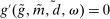 for banks with
  , we obtain

 . Furthermore, since we know that
  for banks with
  , then there is no surplus available in the Fed funds market.
Case 5. Assume that  . We now have that
  for
for  . Thus, if we substitute this result in (44), we obtain

 for banks in surplus, we have that

 . Furthermore, if the condition holds with equality, it must be that
  for banks with
  , and hence, there is no surplus available in the Fed funds market. However, if the condition is strict, then there must be a positive mass of banks with surplus (the supply of government bonds by deficit banks
  does not exceed the holdings of reserves of banks in surplus
 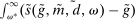 . Consider the special cases where
  , no bank has an initial deficit. Thus, all banks must end with a surplus, and this means we are in Case 5, since this is the only case where this is possible. Q.E.D.
C.3 Proof of Corollaries C.2 and C.3
Proof of Corollary C.2.Assume that there is an aggregate deficit of reserves. Then assume by contradiction that
 (55)
(55)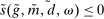 . Hence, we have a contradiction. This rules out Case 1. Now assume that the condition holds with equality. The only possibility is that
  and
and  . This case rules out 2 since
  and F is not degenerate. Hence, the only two scenarios are Cases (3) or (4). Q.E.D.
Proof of Corollary C.3.The result is immediate after we set  in the statement of Corollary C.2. Q.E.D.
C.4 Proof of Items (ii)–(iv)
Auxiliary Lemmas
The proofs of items (ii)–(iv) of Proposition 7 make use of the following two lemmas.
Lemma C.2.The function  is homogeneous of degree 1 in
  .
.
Proof.We need to show  for any
  . By definition,
 (56)
(56) and
and  are functions of
  and independent of m and d. We can factor the constant k from the right-hand side of (56) and obtain

 given by

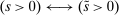 ,
,  and
and  . Thus,

The next lemma establishes that an increase in the (gross) nominal policy rates by a constant scales  by that constant. We use this lemma in the policy analysis results when we discuss the neutrality of inflation.
Lemma C.3.Let  be given by two policy rates,
  , given
  . Consider alternative rates
  such that they satisfy
  and
and  for some k. Then the
  associated with
  for the same
  satisfy
  .
.
Proof.Observe that  in Definition 2 is a function scaled by the width of the corridor system
  . Then

 in Proposition 1. Q.E.D.
Proofs of items (ii)–(iv) of Proposition 7.This section presents a proof of items (ii)–(iv) in Proposition 7. Item (ii) establishes that the single state representation of the value function satisfies homogeneity. We follow the guess-and-verify approach. We guess that the value function satisfies  , where
  is a time-varying scaling factor. From item (i), the bank's problem is summarized by

 , we have that
  can also be written as
 (57)
(57) .
.If the conjecture for the value function is correct, then the value function satisfies


 in (57), we obtain
 (58)
(58)
 ,
,  ,
,  , and
, and  , as in the statement of Proposition 7. By Lemma C.2, we can factor constants
  from
from  and express it as

 in the value function to obtain
 (59)
(59)
 from both sides of (59), which verifies that the objective is scaled by
  . Thus, we verify that
  .
.Next, we derive the policies that attain  and the value of
  . If the conjecture is correct, using the definition of
  , ā, and
  , we obtain
 (60)
(60)
 must be consistent with the solution of
  if the conjecture is correct. Define real return on equity as follows:


 be the certainty equivalent of the bank's optimal portfolio problem, that is,

 and
and  . Assume
  is optimal. If
  , the solution that attains
  must maximize
  if
if  is positive. If
  , the solution that attains
  must minimize
  if
if  is negative. We guess and verify that, indeed, when
  , the term
  is positive and
  is negative when
  . Under this guess, if
  then
then  . Thus, by maximizing
  , we are effectively maximizing the right-hand side of
  . Instead, when
  , then we have that
  . Thus, by maximizing
  , we are minimizing
  , which multiplied by a negative number,
  , maximizes the right-hand side of
  .
.Hence, the Bellman equation becomes

 inherits the sign of
  .
.To prove item (iii), we take the first-order conditions with respect to  , and raising both sides to the
  power, we obtain

 (61)
(61) . Under the conjectured sign of
  , the term
  is always positive. Substituting this expression for dividends, we obtain a functional equation for the value function


 inherits the sign of
  . Thus, we can use
  directly in the value function. Furthermore,
  satisfies the following difference equation:
 (62)
(62)This concludes the proof of items (i)–(iv), for all cases except  . We work out that case next.
Log-Case. Take  . We guess and verify that


 , we have from (61) that
  . In addition,

Appendix D: Proof of Proposition 8
In this section, we suppress time subscripts and study the liquidity premia that emerge from the portfolio problem (16). The calculations here provide the proof for Proposition 8. We derive the premia in the case where government bonds are not large enough to eliminate the surplus of reserves, as in the paper. A more general statement follows simply by substituting  for the corresponding coefficients given in Proposition C.5—everything else remains the same.
 into the objective in (16), to obtain

 be the threshold shock that makes
  . Partition the expectation inside the objective into two terms:

Derivatives of the Liquidity Cost Function


Derivation of the Loan Liquidity Premium
 is interior, we take the derivative with respect to
  to obtain

 , the second line in the expression vanishes. The expectations operator in
  excludes the point
  —since this is a zero probability event, we simply exclude the point where the derivative is not included in the notation. We rearrange terms to express the condition as


 and marginal utility is positive, the loan premium is positive. Finally, since we know that
  , we have that
  . This condition implies that
  .
.Derivation of the Bond Liquidity Premium
In the proof of Proposition 7, item (i), Proposition C.4 shows that when  , we have that
  . If the equality is strict, we also showed that
  . Observe again that since
  , we have that
  . The inequalities are strict if and only if the Fed eliminates the spread in its corridor rates,
  , or if banks are satiated with reserves
  .
.
Derivation of the External Financing Premium and the Deposit Liquidity Premium
 (63)
(63)


 stands for a deposit risk premium:


 marginal utility is decreasing, the risk-weighted expectations operator carries a premium over a fair bet: