Household Leverage and the Recession
Abstract
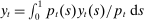
We evaluate and partially challenge the household leverage view of the Great Recession. In the data, employment and consumption declined more in U.S. states where household debt declined more. We study a model of a monetary union composed of many regions in which liquidity constraints shape the response of employment and consumption to changes in debt. We estimate the model with Bayesian methods combining state and aggregate data. Changes in household credit explain 40% of the differential rise and fall of employment across states, but a small fraction of the aggregate employment decline in 2007–2010. Nevertheless, since household deleveraging was gradual, credit shocks greatly slowed the recovery.
1 Introduction
A salient feature of the Great Recession is that U.S. regions with the largest declines in household debt had the largest declines in employment and consumption. Figure 1 illustrates this pattern, originally documented in a series of papers by Mian and Sufi.1 One interpretation of this evidence that has received a lot of attention is the household leverage view of the recession. According to this view, declines in household debt forced households to reduce consumption and, because of price rigidities and trade frictions, caused a reduction in employment.

State debt, employment, and spending.
Our goal in this paper is to quantitatively evaluate the household leverage view of the recession. We ask: how important were shocks to household credit in generating fluctuations in employment and consumption across regions and in the aggregate? The evidence in Figure 1 does not directly answer this question for at least two reasons. First, a variety of shocks, in addition to credit shocks, affect the economy. Second, the response of employment or consumption in an individual state to credit shocks may be very different than the response in the aggregate. Extrapolating from the cross-sectional to the aggregate elasticity requires a careful consideration of trade patterns and monetary policy.
We therefore use a model to isolate the effects of credit shocks and answer our question. We study a tractable model of a monetary union composed of many regions that trade. Households face liquidity constraints that restrict their ability to use the equity in their homes to finance consumption. These constraints generate a time-varying spread between the equilibrium interest rate and the households' rate of time preference. In our baseline model, we assume that credit shocks affect loan-to-value constraints which limit the amount of housing equity that households can extract. In an extension, we obtain similar results by assuming instead that household debt fluctuates in response to credit supply shocks. In addition to credit shocks, households are subject to additional disturbances to productivity and preferences.
We estimate the model using Bayesian full-information methods and data on employment, consumption, wages, house prices, and household debt at the regional and aggregate levels. An important challenge that arises in our estimation is that the policy interest rate was at the zero lower bound (ZLB) during part of our sample. We account for the non-linearities arising from this bound by using a piecewise linear solution method.2 Even with this approximation, a direct application of full-information methods is infeasible in our setting given the large number of regional and aggregate state variables. We therefore develop a methodology that allows us to combine regional and aggregate data to evaluate the likelihood function.
A popular approach to modeling household debt is to assume heterogeneity in agents' rate of time preference, as in Iacoviello (2005) and a large literature that follows.3 These models feature a single financial asset, which impatient households use to borrow from patient households. A tightening of credit limits reduces the amount that impatient households borrow and translates into a dollar-for-dollar drop in their consumption, but, in the absence of changes in the equilibrium interest rate, leaves patient households unaffected. Such models thus predict that consumption in an individual region changes dollar-for-dollar with changes in household debt, regardless of how many agents are impatient, as long as the region is sufficiently small so it does not affect the economy-wide interest rate. One-asset models therefore imply counterfactually large comovements between consumption and credit across regions, at odds with the evidence in Figure 1.4
Motivated by this observation, we pursue an alternative approach. We assume that households are subject to idiosyncratic shocks to their liquidity needs which make it optimal to simultaneously hold liquid assets and borrow. A household can therefore respond to a tightening of credit by drawing on its liquid assets instead of cutting consumption. The extent to which it can do so depends on the volatility of idiosyncratic shocks. If these shocks are volatile, the household maintains its liquid asset position, thus reducing consumption sharply after a credit tightening. If, in contrast, the volatility of idiosyncratic shocks is low, households find it optimal to dip into their liquid assets to insulate consumption from credit shocks. Our model thus flexibly nests both one-asset models in which a region-specific tightening of credit leads to a large drop in consumption, as well as the frictionless model in which credit shocks have no effect on consumption. We view this framework as our main theoretical contribution: it is flexible enough to capture complex credit dynamics but simple enough to be estimated on a full panel of regional economic data.
We next explain why households in our model value liquidity. The typical approach to modeling the notion that housing equity is illiquid is to assume that agents must pay a fixed cost to refinance their mortgage, as in the work of Kaplan, Mitman, and Violante (2020) and Boar, Gorea, and Midrigan (2020). Since most homeowners who do not refinance are constrained,5 they save in a liquid asset in order to smooth consumption. By contrast, considerations of computational tractability lead us to follow an alternative approach inspired by Lucas (1990). Agents in our model can costlessly rebalance their portfolios between periods, but they must do so prior to the realization of an idiosyncratic preference shock. We achieve tractability by assuming a family construct to eliminate the distributional consequences of asset market incompleteness.6 These assumptions allow us to parsimoniously model an interest-elastic supply of liquid assets of the type that would arise in richer but less tractable models of mortgage refinancing. In particular, the larger the interest rate is relative to the rate of time preference, the more households save in their liquid accounts to smooth the impact of idiosyncratic shocks. Our notion of liquidity therefore closely resembles that in the work of Shi (2015), Rocheteau, Weill, and Wong (2018), and Kiyotaki and Moore (2019) in which liquidity is valued because of idiosyncratic investment opportunities or preference shocks.
Consider now the macroeconomic implications of a credit shock. At the economy-wide level, a tightening of credit leads to a reduction in the natural interest rate. The drop in the natural rate depends on the volatility of idiosyncratic preference shocks: more volatile shocks reduce the elasticity of liquid assets and imply a larger fall in the natural rate. If prices are sticky and monetary policy is unable to track the natural rate, the credit shock leads to a decline in employment. The response to economy-wide credit shocks is therefore highly non-linear depending on how long the ZLB is expected to constrain monetary policy. At the regional level, a tightening of credit acts like a sudden stop by forcing an increase in the net foreign asset position, as in Gourinchas, Philippon, and Vayanos (2016), but the extent of the increase in net foreign assets depends, once again, on the volatility of idiosyncratic shocks. Hence, the same parameter governing the elasticity of liquid assets determines both the economy-wide and regional implications of a tightening of credit, a feature that we exploit in estimation.
We estimate three structural parameters that play a key role in shaping the economy's response to a credit shock: the degrees of wage and price stickiness, and the degree of idiosyncratic uncertainty. We also estimate the persistence and volatility of the regional and aggregate shock processes. To make full-information estimation feasible, we exploit the structure of the model and express regional variables as deviations from the corresponding aggregates. Up to a first-order approximation, these deviations evolve independent of monetary policy. This structure allows us to separate the likelihood function into independent state-level and aggregate components. Intuitively, our estimation exploits the differential rise and fall of individual states' spending, employment, debt, wages, and house prices, in addition to the aggregate comovement of these series, to identify the structural parameters.
We use the model to generate counterfactual series for employment and consumption by turning off all shocks other than credit shocks. We find that credit shocks alone account for 40% to 50% of the relative movements in state-level employment and consumption during the 2002 to 2010 period. Our findings are thus consistent with those of Mian and Sufi (2011, 2014).
We next discuss the model's economy-wide implications. We distinguish between two periods: the onset of the Great Recession from 2007 to 2010, and the recovery period up to the end of 2012. Given the non-linear nature of the responses at the ZLB, we provide bounds on the impact of credit shocks. The lower bound assumes no ZLB. The upper bound assumes that the ZLB binds and that the Fed does not pursue forward guidance. Under both bounds, we find that household credit shocks have a relatively small impact on employment between 2007 and 2010. In the data, employment fell by 7% during this period. In contrast, the lower and upper bounds on the contribution of credit shocks to the decline in employment are 0.5% and 1.7%, respectively. Thus, even under the stark assumption that the Fed did not react to credit shocks at all, household deleveraging explains at most a quarter of the drop in employment during the acute phase of the crisis. This result is a consequence of the gradual nature of household deleveraging which leads to a gradual decline in the natural rate and reflects the findings of Kaplan, Mitman, and Violante (2020) who showed that the duration of mortgages greatly matters for the effects of shocks to household credit.7
The results are different when we consider the period 2007 to 2012. Since household debt fell more over this longer period, so did the natural rate, and the model predicts a more important role for credit shocks. In the data, employment was 6.2% lower by the end of 2012 compared to 2007. Under the two bounds, employment declined by 1.3% and 4.8%, respectively. The model therefore predicts that credit shocks greatly delayed the recovery.8 As we show in the Supplemental Material (Jones, Midrigan, and Philippon (2022)), our results are robust to a number of perturbations, including adding a construction sector, allowing for fiscal policy, lowering the duration of mortgage contracts, explicitly modeling mortgage default, credit supply shocks, and heterogeneity in state responses to credit shocks.
Our goal in this paper is to quantify the role of credit shocks in accounting for regional and aggregate employment during the Great Recession. To keep our analysis as transparent as possible, we focus on the household leverage view of the Great Recession and do not explicitly model the other forces that arguably played an important role, such as bank and firm-level financing constraints, changes in uncertainty, demographics, increase in markups, and risk premia. These factors are instead captured by our rich set of exogenous shocks. A limitation of our approach is that household credit may interact with a number of these forces in important ways.9
Our analysis also focuses on a representative agent economy, which, in general equilibrium, precludes us from capturing housing wealth effects on consumption. Introducing housing wealth effects, which Kaplan, Mitman, and Violante (2020) argued were responsible for a large fraction of the expenditure drop during the Great Recession, requires explicitly modeling household heterogeneity and the resulting correlation between wealth effects and marginal propensities to consume across households. To keep our analysis tractable, we abstract from such heterogeneity and thus implicitly capture these forces using changes in the household's rate of time preference.
Our paper is related to Eggertsson and Krugman (2012) and Guerrieri and Lorenzoni (2017) who also studied the responses of an economy to a household credit crunch. While they studied a closed economy, our model is that of a monetary union composed of a large number of regions. Moreover, our focus is on estimating the model using state and aggregate data. Since we found that one-asset models cannot account for the comovement between state-level consumption and household debt, we explicitly introduce liquidity constraints which make it optimal for households to simultaneously borrow and save in the liquid asset, an ingredient which we argue is critical to match the regional data.
Our use of regional data in estimation is related to Beraja, Hurst, and Ospina (2019) who applied a limited-information approach to estimate the degree of wage stickiness using state-level data, and then used those estimates as a prior in a full-information estimation with aggregate data. In contrast, our methodology simultaneously uses regional and aggregate data in a full-information approach, despite the large number of state variables and non-linearities caused by the ZLB. Our emphasis on cross-sectional evidence is also shared by the work of Nakamura and Steinsson (2014). Finally, our work is related to the literature on financial intermediation, originating with Bernanke and Gertler (1989), Kiyotaki and Moore (1997), Bernanke, Gertler, and Gilchrist (1999), and more recently, Mendoza (2010), Gertler and Karadi (2011), Gilchrist and Zakrajšek (2012).10
2 Model
We first describe the model economy. The economy consists of a continuum of ex ante identical islands of unit mass that belong to a monetary union and trade among themselves. Consumers derive utility from a final good, leisure, and housing. The final good is assembled using as inputs traded and non-traded goods. We assume that producers of intermediate goods are monopolistically competitive. Prices and wages are subject to Calvo adjustment frictions. Labor is immobile across islands and the housing stock on each island is in fixed supply.
We explicitly model the distinction between liquid and illiquid assets on households' balance sheets. In contrast to Kaplan and Violante (2014) and much of the segmented asset markets literature which assumes fixed costs of portfolio rebalancing, we formulate an alternative approach following Lucas (1990). We assume that consumers allocate their wealth between liquid and illiquid assets prior to the realization of an idiosyncratic preference shock. The more volatile this shock is, the stronger the precautionary savings motive in liquid assets, and the larger the response of consumption to credit shocks. Following Lucas (1990), we assume that consumers belong to families that share idiosyncratic risks.
Households face shocks to their ability to tap home equity, which we refer to as credit shocks. We also allow for shocks to the households' rate of time preference, disutility from work, preference for housing, and productivity. Each shock has an island-specific and aggregate component. We also assume aggregate shocks to the interest rate rule and to the aggregate inflation equation. These additional shocks capture other channels that can explain movements in macroeconomic aggregates.
2.1 Households
Securities
Households borrow using mortgages, which are long-term perpetuities with coupon payments that decay geometrically at a rate determined by a parameter γ. A seller of such a security issues one unit at a price  in period t and repays 1 unit of the good in period
  , γ units in
  ,
,  in
in  , and so on in perpetuity.11 The household borrows from perfectly competitive financial intermediaries.
 it must make in period t. Letting
  denote the amount of newly issued mortgages in period t, the date
  coupon payments are

 denote the economy-wide price of one claim to such a perpetuity, the value of a household's mortgage liabilities is
  , reflecting the amount the household owes in coupon payments in period t and the market value of its outstanding debt. On the asset side, we assume that households save in a one-period nominal security at a rate
  .12
.12Preferences

 denotes the consumption of a member i of household
  ,
,  denotes the total amount of housing owned by that household, and
  denotes the labor it supplies. The shifters
  and
and  determine the preference for housing and the disutility from work, while
  is the household's one-period-ahead discount factor. Each of these preference shifters has an island-specific and an aggregate component, all of which follow AR(1) processes with independent Gaussian innovations.
 is specific to each consumer i and denotes an idiosyncratic taste shifter, which is an i.i.d. random variable drawn from a Pareto distribution

 determines the amount of uncertainty about v. A lower α implies more uncertainty. Below, we drop the dependence on ι for notational simplicity.
Budget and Credit Constraints
 denote the total amount of funds the household transfers to its members. We assume that
  is chosen prior to the realization of the idiosyncratic preference shock
  . Since individual members are ex ante identical and of mass 1,
  also represents the amount of funds received by any individual member. We assume a liquidity constraint which limits each member's consumption by the amount of funds it has when entering the goods market:
 (1)
(1) is the price of the final good on island s. The budget constraint is
 (2)
(2) is the price of housing,
  is the wage rate the household faces,
  are the coupon payments on outstanding mortgage debt,
  are the liquid assets it enters the period with, and
  collects the profits households earn from their ownership of intermediate goods firms, transfers from the government aimed at correcting the steady-state markup distortion, as well as the transfers stemming from the risk-sharing arrangement. We assume that households on island s exclusively own firms on that island.
 (3)
(3) evolves as the product of an island-specific and an aggregate component, both of which follow an AR(1) process. This formulation allows us to capture the slow movement of debt in the data in which only a fraction of households obtain new mortgages in any given period, and so face the current credit conditions and house prices in determining mortgage limits.
We introduce housing preference shocks to capture movements in house prices that are otherwise difficult to rationalize.13 Because housing is separable in the utility function and the housing stock is in fixed supply, movements in house prices only affect equilibrium allocations via their impact on the households' ability to borrow.14 Specifically, a housing preference shock that increases house prices loosens the borrowing constraint (3) and leads to an increase in consumption.
Savings

 .
.Our model is reminiscent of cash-in-advance models, though there are several important differences. First, we assume that the household can access its date t labor income  immediately. Second, we allow agents to save in interest-bearing assets at the conclusion of their shopping period. The only distortion we introduce is that arising from the household's inability to smooth the marginal utility of consumption across its members within a period.
Timing
Figure 2 summarizes our timing assumptions. The household's portfolio composition is described by liquid assets  , housing
  , and mortgage debt
  . All shocks except
  are realized at the beginning of the period. The household then chooses labor
  , housing
  , borrowing
  , and transfers
  . The idiosyncratic preference shocks
  are then realized and individual members choose consumption
  . All unspent funds
  are then saved in the liquid asset.

Timing of the model.
2.2 Optimal Savings Choice
 denote the multiplier on the household's budget constraint (2) and
  denote the multiplier on the liquidity constraint (1). The choice of
  satisfies
 (4)
(4) is valued at
  , the shadow value of wealth. Since unspent funds can be saved at the conclusion of the shopping period, they are valued at
 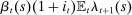 . The last term captures the liquidity services provided by
  , namely the average multiplier on the liquidity constraint of individual members.
 (5)
(5) (6)
(6)

 , they can be expressed as
 (7)
(7)To understand this expression, note that when  is high, the household is relatively impatient. Idiosyncratic taste shocks generate a precautionary savings motive, in addition to the intertemporal substitution motive. When uncertainty about taste shocks is high (α is low), the precautionary motive dominates so savings are relatively insensitive to the wedge
  . In contrast, when the uncertainty about taste shocks is low (α is high), the precautionary motive is weak and savings are sensitive to
  . As
. As  , the supply of liquid assets is infinitely elastic.
The assumption that taste shocks are Pareto distributed, or that idiosyncratic uncertainty takes the form of preference, as opposed to income or expense shocks, is not critical to our arguments. In the Supplemental Material, we consider alternative types of shocks. Although these alternatives are not as tractable as our baseline formulation, their qualitative implications are similar.
2.3 Optimal Debt and Housing Choice

 is
is
 (8)
(8) is the multiplier on the borrowing constraint (3). The first-order condition for housing is
 (9)
(9)2.4 Technology
We next discuss the assumptions on technology we make.
Final Goods Producers
 units of the final good using
  units of non-tradable goods produced locally and
  units of imported goods. Imported and non-tradable goods are combined using a CES aggregator with elasticity of substitution σ,


 is the price of imports from island s. Letting
  denote the price of non-tradable goods, the final goods price on an island is


Intermediate Goods Producers
 that is common to both the tradable and non-tradable sectors:

 each period. A firm that resets its price maximizes the present discounted flow of profits weighted by the probability that the price it chooses at t will still be in effect at any particular date. The government levies a production subsidy
  which eliminates the steady-state markup distortion and is financed with lump-sum taxes.
Wage Setting
Households are organized in unions that supply differentiated varieties of labor with elasticity of substitution ψ. Unions reset their wages with probability  each period. We assume that the government offsets the steady-state wage markup distortion using a subsidy
  financed with lump-sum transfers.
2.5 Monetary Policy
 be total output in this economy,
  be the aggregate price level, and
  denote the rate of inflation. Aggregating the prices of individual producers in all islands implies, up to a first-order approximation,

 is the average wage in the economy,
  is an AR(1) disturbance to individual firms' desired markups, common to all islands,
  is the steady-state discount factor and
  is the steady-state rate of inflation.15
 is the steady-state nominal interest rate,
  is an i.i.d. monetary policy shock,
  determines the persistence, and
  ,
,  , and
, and  determine the extent to which monetary policy responds to deviations of inflation from the target
  , the output gap
  , and the growth rate of the output gap, respectively. The output gap is the ratio of output to its flexible-price level. When the ZLB binds,
  .
.The Fed may set an interest rate of zero not only when the ZLB binds, but also when it follows its forward guidance. In particular, we assume that, in periods in which the ZLB binds, the Fed can commit to keeping  at zero for longer than the duration prescribed by the Taylor rule. We thus implicitly assume that the Fed can manipulate expectations of how the path of interest rates evolves when the economy hits the ZLB, as in Eggertsson and Woodford (2003) and Werning (2011). In our estimation, we use survey data from the New York Federal Reserve to discipline the expected duration of the zero interest rate regime between 2009 and 2015.
2.6 Asset Market


We next discuss the role of liquidity constraints in determining the steady-state equilibrium interest rate. Recall that the household's liquid savings are given by (7). In steady state, the wedge between the discount rate and the interest rate is equal to  , where
  is the discount rate and
  is the real interest rate. The upward-sloping curves in Figure 3 illustrate the households' optimal savings choices as a function of the real interest rate. The two panels of the figure correspond to two scenarios, one with a relatively high idiosyncratic uncertainty (low α), and another with a relatively low uncertainty (high α).

Equilibrium real interest rate in steady state.
To derive the demand for assets, we note that the borrowing limit binds at all times. This is because taste shocks are unbounded, which implies that the multiplier on the liquidity constraint  is positive for a positive mass of household members. A comparison of (4) and (8), together with the no-arbitrage condition
  , implies that the multiplier on the borrowing constraint
  is also positive. Intuitively, since the household anticipates that a fraction of its members will end up liquidity-constrained, and since the expected return on the mortgage is equal to the liquid interest rate, it borrows as much as possible. The result that all households are constrained, though stark, is consistent with Boar, Gorea, and Midrigan (2020) who found that four-fifths of homeowners are debt-constrained.16
 (10)
(10) , discounted by a weighted average of the rate of time preference ρ and the interest rate r, with a weight that depends on how much the household can borrow. As long as
  , an increase in the loan-to-value ratio
  reduces the effective discount rate, raising house prices.
The downward-sloping curve in Figure 3 superimposes the demand for mortgages (10) and illustrates how the equilibrium interest rate is determined in steady state. A tightening of the debt limit mechanically reduces the demand for debt, thus reducing the equilibrium interest rate. The extent to which the equilibrium interest rate falls depends on the degree of idiosyncratic uncertainty. As the two panels of the figure show, the larger the uncertainty, the less elastic the supply of liquid assets, and therefore the larger the reduction in the equilibrium interest rate.
2.7 The Workings of the Model
We next provide some intuition for how the model works. The key parameters in the model are those that determine the degree of idiosyncratic uncertainty, α, and those governing the degree of price and wage stickiness,  and
and  . We illustrate the role of each of these sets of parameters by perturbing them and describing the impulse responses to shocks to the credit limit
  .
.
Impulse Response to a State-Level Credit Shock
Figure 4 reports impulse responses to a state-level credit shock. To build intuition, we first report, in the left column, the responses under flexible prices. Panel A of the figure shows that the shock leads to a gradual decline in debt because of the long-term nature of mortgages. Households cannot borrow as much as they used to, and they respond in three ways. They reduce their liquid asset holdings, which limits their ability to smooth idiosyncratic shocks. They also reduce consumption and increase labor supply. Prices and wages fall, employment rises, and the island runs a current account surplus.

Impulse response to state-level credit shock.
The middle column of Figure 4 illustrates how price rigidities affect the response of an island to a credit shock. We refer to this parameterization as the “Baseline” because it relies on the parameters from our estimation below. Wage and price rigidities reverse the response of employment. Price stickiness limits the increase in exports so the increase in the current account takes place via a compression of domestic demand. The fall in employment reduces income and consumption further. Wage rigidities act as a tax on labor supply, while price rigidities increase firms' markups, and both effects reduce employment.17
The last column of Figure 4 illustrates how liquidity constraints and liquidity demand affect the response of an island to a credit shock. We reduce the volatility of idiosyncratic shocks by increasing the parameter α. With less need to smooth large liquidity risks, households are more willing to reduce their liquid asset holdings in response to a tightening of their borrowing limit. As a result, consumption barely falls and the impact on employment and wages is small. These effects are captured in equation (7) which shows that liquid asset holdings are more sensitive to the wedge between the discount rate and the interest rate when α is high. The discount rate  increases in response to the credit tightening, while the interest rate is constant since the island is atomistic. When idiosyncratic uncertainty is low, it is relatively costless to reduce liquid asset holdings. Both sides of the household's balance sheet thus contract, with little impact on other variables. In this case, credit is a veil with little impact on macroeconomic aggregates. In contrast, when idiosyncratic uncertainty is high, reducing liquid assets is costly. Households therefore find it optimal to respond to the credit tightening by cutting consumption.
A tightening of debt constraints thus distorts allocations in two ways: it prevents households from smoothing the marginal utility of consumption both across members and across time. Households face a tradeoff: they can respond to a tightening of credit by either reducing overall consumption, distorting the intertemporal allocations, or by reducing liquid assets, distorting the intrafamily allocations. The more dispersed idiosyncratic shocks are, the more the household reduces overall consumption to limit variation in the marginal utility of consumption across its members.
Impulse Response to an Aggregate Credit Shock
 is approximately inversely proportional to nominal consumption spending,
  . Up to a first-order approximation, the Euler equation that determines the growth rate of
  is given by

 (11)
(11) , thus reducing the natural rate.
The first column of Figure 5 shows the response to an aggregate credit shock in an economy with flexible prices. The shock reduces the interest rate (Panel A), and has a negligible effect on employment (Panel D). Employment falls slightly because a tightening of credit magnifies consumption-leisure distortions, as in cash-in-advance economies where the impact of these distortions is small (Cooley and Hansen, 1989).

Impulse response to an aggregate credit shock.
We next turn to our baseline parameterization with sticky prices. As is well understood, the extent to which changes in the natural rate affect macroeconomic aggregates depends on the stance of monetary policy. We illustrate this point in the second column of Figure 5 by contrasting the responses to the same credit shock under two scenarios: one in which we impose the ZLB and another one in which we do not. Clearly, the ZLB magnifies the reduction in employment because it prevents the monetary authority from accommodating the decline in the natural rate.
As with the island-level responses, the volatility of idiosyncratic shocks is critical in determining how the economy reacts to a credit shock. As the last column of Figure 5 shows, if idiosyncratic uncertainty is low, interest rates and employment fall little. In this case, liquid asset holdings are sensitive to interest rates, so a small reduction in the equilibrium rate is required to clear the asset market. The natural rate of interest thus falls little, leading to a negligible impact on macroeconomic outcomes.
This exercise shows that the parameters that shape the responses of island-level variables to credit shocks also determine the aggregate-level responses. These parameters govern the slopes of two curves: that of the Phillips curve that relates inflation to changes in marginal costs and that of the savings curve which relates liquid asset holdings to the gap between the discount rate and the interest rate. Since these are both functions of the primitive parameters, they are identical in the aggregate and at the state level. In contrast, the equilibrium responses of, say, employment to credit shocks are determined by factors such as a state's openness to trade and the stance of monetary policy and one cannot extrapolate state-level elasticities to draw conclusions about the aggregate. Indeed, if monetary policy perfectly tracked the natural rate, it would eliminate aggregate employment fluctuations, yet would be unable to respond to disturbances on an individual island. We can therefore use state-level data to identify the parameters that determine the slopes of these curves, but need to use the structure of the model to identify the aggregate impact of credit shocks.
Our modeling of how households allocate their wealth between housing, liquid assets, and mortgage debt is purposefully simple and designed to capture aggregate comovements, not the behavior of individual households. Just as the Calvo pricing protocol is a crude description of how individual firms price, our family construct is a crude description of how households save. Fully micro-founding household portfolio choices would require a rich three-state model of the housing market similar to that studied by Kaplan, Mitman, and Violante (2020) and Boar, Gorea, and Midrigan (2020). Such a model would entail significant micro-level non-convexities that would make full-information estimation infeasible. Since our goal is to use state-level data to isolate the impact of monetary policy in stabilizing the response of real variables to credit shocks, our conjecture is that our simplification provides a useful approximation, analogous to the Calvo pricing approach in modeling the dynamics of inflation.
2.8 Solution Method
To use Bayesian techniques in estimation, we need an efficient solution method. We thus use a piecewise linear approximation method developed by Eggertsson and Woodford (2003), Guerrieri and Iacoviello (2015), and Jones (2017) to deal with the ZLB. We next describe the method, which we adapt for our application combining state-level and aggregate variables.

 is a vector that collects state-level variables,
  are the state-level shocks,
  are the aggregate variables,
  are the aggregate shocks, and the bold matrices are functions of the parameters of the model.
The economy may be in one of two regimes. Let  denote periods when the ZLB does not bind, and
  periods when it does. Because each individual island is atomistic, whether the ZLB binds does not, up to a first-order approximation, affect the dependence of an island's variables on its own lagged or future variables, or its shocks. Thus, the matrices A, B, D, and F are not regime-dependent.
 , and adding the Taylor rule, we derive the dynamics of aggregate variables as

 collects all the aggregate variables,
  , and the nominal interest rate
  . Notice that the coefficient matrices depend on the monetary policy regime.
 , under the assumption that agents observe all shocks in each period, but believe that no other shocks are possible in the future. Under the regime when the ZLB does not bind, we use standard methods to derive the time-invariant VAR representation of the aggregate variables
 (12)
(12) at which the ZLB will stop binding conditional on no further aggregate shocks hitting the economy. Here
  encodes forward guidance announcements, if any. For periods after T, the economy evolves following (12). Prior to T, the solution of the model is
 (13)
(13) (14)
(14)
 . We iterate on the conjectured date T until convergence.18
 (15)
(15) ,
,  , and
, and  encode how an island responds to aggregate-level variables and vary over time because of the ZLB. In contrast, the matrices Q and G, which determine how an island's variables depend on their own lags and island-specific shocks, are time-invariant. Intuitively, since each island is of measure zero, shocks to an individual island do not change the expected date at which the ZLB will stop binding for the rest of the economy. Moreover, agents on each island take aggregate prices, including the interest rate, as given. Therefore, conditional on the aggregate state variables, the ZLB regime does not affect the evolution of island-level relative variables. From the perspective of agents on a given island, the presence of the ZLB acts like any other aggregate shock which, up to a first-order approximation, does not change how that island responds to its own history of idiosyncratic shocks.
Equation (15) reveals that our model has a special structure. First, the mapping from state-level histories of shocks to state-level outcomes is time-invariant and common to all states. Second, the mapping from aggregate histories of shocks to state-level variables, though time-varying, is also common to all states. We exploit this structure to construct the likelihood function, as we describe below.
3 Estimation
We next explain how we chose parameters for our model. We first discuss the parameters we assign values to, and then the ones we estimate. The parameters that we estimate are those that are critical in determining the model's responses to a credit shock: the degree of wage and price stickiness,  and
and  , as well as the volatility of idiosyncratic taste shocks, α. We refer to these parameters as our structural parameters. In addition, we estimate the AR(1) processes characterizing the island-specific and aggregate components of the various shocks. We next describe the parameters we have assigned, the construction of the likelihood function, and then our results.
3.1 Assigned Parameters
We report the parameter values we assign in Table I. The period is one quarter. We assume a Frisch elasticity of labor supply of 1/2. We set γ, the parameter governing the duration of debt, to 0.985, so that the Macaulay duration of debt in our model is equal to that of 30-year mortgages, approximately 13 years.19 We follow the trade literature in setting the weight on non-traded goods in an island's consumption basket, ω, equal to 0.7; the elasticity of substitution between tradable and non-tradable goods, σ, equal to 0.5; and the elasticity of substitution between varieties of tradable goods produced in different islands, κ, equal to 4, the estimate of Simonovska and Waugh (2014). We follow Christiano, Eichenbaum, and Evans (2005) in choosing ψ to ensure a wage markup of 5%.20 We use the Justiniano, Primiceri, and Tambalotti (2011) estimates of the Taylor rule.
|
Parameter |
Value |
Description |
Source/Target |
|---|---|---|---|
|
ν |
2 |
Inverse labor supply elasticity |
|
|
γ |
0.985 |
Persistence coupon payments |
13 year mortgage debt duration |
|
ω |
0.7 |
Weight on non-traded goods |
|
|
σ |
0.5 |
Elasticity traded/non-traded |
|
|
κ |
4 |
Elasticity traded goods |
|
|
ψ |
21 |
Elasticity labor aggregator |
|
|
αr |
0.86 |
Taylor rule persistence |
|
|
απ |
1.71 |
Taylor coefficient inflation |
|
|
αy |
0.05 |
Taylor coefficient output |
|
|
αx |
0.21 |
Taylor coefficient output growth |
|
|
Parameters chosen to match steady-state target |
|||
|
−ln(β) |
2.46% |
Annual discount rate |
2% real rate |
|
η |
0.084 |
Weight on housing |
Housing-to-income ratio of 2.5 |
|
|
0.0044 |
Credit limit |
Debt-to-housing ratio of 0.29 |

We pin down three additional parameters using steady-state considerations. The steady-state discount factor  is chosen so that the steady-state real interest rate is equal to 2% per year. The steady-state weight of housing in preferences
  is chosen so that the aggregate housing to (annual) income ratio is equal to 2.5, a number that we compute using the 2001 Survey of Consumer Finances (SCF). Finally, the steady-state LTV ratio is chosen so that the aggregate debt to housing ratio is equal to 0.29, a number once again computed from the SCF. Since the debt constraint binds, these last two targets imply an aggregate debt to (annual) income ratio of
  .
.
3.2 Estimation Procedure
Our goal is to simultaneously use regional and aggregate data to estimate the model and identify the impact of credit shocks on real activity. In contrast to Nakamura and Steinsson (2014) and Beraja, Hurst, and Ospina (2019), who also used regional data to understand the effect of various shocks on macroeconomic aggregates, our approach simultaneously uses state and aggregate-level data in a full-information estimation. One important technical challenge we need to overcome in order to compute the likelihood function is the presence of the occasionally binding ZLB, which renders conventional methods infeasible due to the very large number of island-level state variables and the resulting curse of dimensionality. We therefore exploit the special structure of our model and develop an efficient algorithm that circumvents these difficulties. We first describe the details of our approach, and then report our results.
3.2.1 The Data
Regional Data

 is the market value of mortgage debt issued in period t and
  is the book value of outstanding debt. We found that our results are unchanged if we instead use the market value of debt
  to proxy for household credit.
We use data on house prices from the FHFA, and data on employment, consumption expenditures, and wages from the BEA. Our measure of employment is the employment-population ratio in a given state. Our measure of wages is total employee compensation divided by the number of workers. Since we do not model the construction sector, we subtract construction employment and compensation in computing measures of employment and wages.22
Aggregate Data
We use aggregate data on employment, household consumption expenditures, wages, household debt, house prices, inflation, and the Fed Funds rate from 1984 to 2015. An additional critical input in the estimation is the sequence of expected durations of the ZLB between 2009 and 2015, which we take from the Blue Chip Financial Forecasts survey and the New York Federal Reserve's Survey of Primary Dealers. The Supplemental Material provides more detail on the data we use.
3.2.2 The Likelihood Function
The conventional approach to estimating the model would be to use a likelihood function that directly combines state and aggregate data. However, this approach is infeasible because of the non-linearity induced by the ZLB and the curse of dimensionality which arises from our use of 51 regions, each of which has 11 state variables.
We thus use the structure of our model to formulate an alternative approach to constructing the likelihood function, one that exploits relative variation across individual states' outcomes. Intuitively, our approach recognizes that, up to a first-order approximation, the difference between employment in, say, Nevada and in the aggregate is a linear function of the Nevada state variables only. This observation allows us to separate the likelihood into state-level and aggregate components.


 (16)
(16)
 is the contribution to the likelihood of an individual state's data,
  is the contribution to the likelihood of the aggregate data, and
  is the relative weight of state s. This additive structure follows from the block structure implied by representation (16) which allows us to express the determinant of the variance-covariance matrix of the forecast errors as the product of the determinants of the variance-covariance matrices of the individual states, as we show in the Supplemental Material.
 the number of observable variables and by
  (1999 to 2015) the number of years of data that are available. With Gaussian errors, the log-likelihood function is

 is the vector of forecast errors, calculated using the Kalman filter and the structural matrices Q and G from (16), and
  is the covariance matrix of
  . We compute the aggregate likelihood component in a similar fashion, taking into account that the sequence of forecast errors and their covariance matrices are functions of the underlying time-varying reduced-form matrices
  and
and  from (13).
To summarize, our estimation exploits the differential rise and fall of individual states' spending, debt, wages, house prices, and employment, in addition to the aggregate comovement of these series, to identify the structural parameters of the model. Notice that by simultaneously using state and aggregate data to construct the likelihood, our approach differs from that of Beraja, Hurst, and Ospina (2019), who first applied limited information methods to estimate the degree of wage stickiness using state-level data. They then used that estimate to form a prior in a second step, which uses only aggregate data to form the likelihood function.
The state-level data are observed at an annual frequency, while the model is quarterly, so we conduct a mixed-frequency estimation, by computing forecast errors every four quarters for state-level variables. The aggregate data, in contrast, are quarterly and for a longer time-period (1984 to 2015). To account for differences in the size of different states and ensure that smaller states exert a relatively smaller influence on the shape of the likelihood, we weight the likelihood contribution of each state by its 1999 population shares. In a robustness exercise reported in the Supplemental Material, we also compute the likelihood under equal weighting. In our baseline, we assign an equal weight to the aggregate likelihood and the combined state-level likelihood.
3.3 Parameter Estimates
Table II reports moments of the prior and posterior distributions of the structural parameters we estimate. We use diffuse priors. We find, consistent with the work of Del Negro, Giannoni, and Schorfheide (2015), that wages and prices are sticky, with a modal estimate of  of 0.96 and a modal estimate of
  of 0.86. As is well known, accounting for the stability of inflation around the Great Recession requires a great deal of price stickiness. We show below that estimating the model using state-level data alone implies a lower degree of price stickiness, consistent with Beraja, Hurst, and Ospina (2019). We show the implications under these alternative parameters in our Supplemental Material.
|
Parameter |
Prior |
Posterior |
|||||
|---|---|---|---|---|---|---|---|
|
Distribution |
Median |
10% |
90% |
Mean |
10% |
90% |
|
|
θp |
Beta |
0.5 |
0.2 |
0.8 |
0.96 |
0.94 |
0.98 |
|
θw |
Beta |
0.5 |
0.2 |
0.8 |
0.86 |
0.82 |
0.89 |
|
α |
Normal |
2.5 |
1.2 |
3.8 |
3.44 |
3.05 |
3.93 |
The mean estimate of the Pareto tail parameter α is equal to 3.44, implying a 0.47% spread between the subjective discount rate and the interest rate at the annual frequency. Notice that this parameter is well identified with a relatively tight posterior distribution. The 10th and 90th percentiles are 3.0 and 3.9, respectively. This estimate implies that the fraction of household members who are liquidity-constrained is relatively low, 0.3% in steady state. Moreover, as we show in the Supplemental Material, the model's implications for the marginal propensity to consume out of a transitory income shock are also very similar to those of the frictionless model. In this sense, our results do not rely on assuming severe liquidity constraints.
The Supplemental Material reports the posterior estimates of the parameters governing the persistence and volatility of state and aggregate shocks, and the time series of shocks.
3.4 Identification of α
We next provide intuition for how the key parameter α is identified from the comovement of state-level household debt, consumption, and employment. Table III reports coefficient estimates from univariate regressions of changes in employment and consumption on changes in household debt in the boom (2002 to 2007) and the bust (2007 to 2010). As pointed out by Mian and Sufi (2014), state-level data show a strong correlation between these variables. For example, as the first column of the table shows, an increase in debt-to-income of 100 percent is associated with a 7 percent increase in employment and 15 percent increase in consumption from 2002 to 2007.
|
Data |
Baseline |
||||
|---|---|---|---|---|---|
|
A. Dependent Variable: Δ Debt. Boom, 2002 to 2007 |
|||||
|
Δ Employment |
0.07 |
0.06 |
0.22 |
0.02 |
0.02 |
|
(0.01) |
(0.01) |
(0.01) |
(0.01) |
(0.01) |
|
|
Δ Consumption |
0.15 |
0.11 |
0.31 |
0.02 |
0.02 |
|
(0.03) |
(0.01) |
(0.01) |
(0.01) |
(0.01) |
|
|
B. Dependent Variable: Δ Debt. Bust, 2007 to 2010 |
|||||
|
Δ Employment |
0.10 |
0.06 |
0.22 |
0.03 |
0.01 |
|
(0.01) |
(0.01) |
(0.01) |
(0.01) |
(0.01) |
|
|
Δ Consumption |
0.17 |
0.10 |
0.31 |
0.03 |
0.02 |
|
(0.02) |
(0.01) |
(0.01) |
(0.01) |
(0.01) |
|


- a Other parameters as in baseline.
- b Other parameters reestimated.
- Note: Standard errors in parentheses.
We next discuss the model's predictions for these comovements. We use our mean estimates in Table II to simulate a large panel of states and run identical regressions in the model. As the second column of Table III shows, our baseline model reproduces the correlations in the data very well. Consider next what happens if we simulate data from the model using higher and lower values of α. When idiosyncratic uncertainty is high  , employment and consumption comove much more strongly with changes in household debt than in the data. For example, a 100 percent increase in household debt-to-income is associated with a 22 percent increase in employment and 31 percent increase in consumption. In contrast, when idiosyncratic uncertainty is low
  , employment and consumption comove little with changes in household debt. For example, a 100 percent increase in household debt-to-income is associated with a 2 percent increase in employment and consumption.
In the Supplemental Material, we report the predictions of our model for the comovement between employment, consumption, and household debt for longer leads and lags using local projections. We show that simulated series from the model with too high or too low values of α generate impulse responses that greatly differ from those computed in the data. We also report in the Supplemental Material that a GMM-based procedure produces similar estimates of α as in our baseline.
3.5 Separating Credit Shocks From Other Demand Shocks
How does our framework identify the separate contribution of shocks that change household credit limits from that of discount factor shocks, which also lead to comovements between consumption and household savings? To see this, recall that we assume that there is no spread between the rate at which households save in the liquid asset and the mortgage interest rate. Since liquid assets provide liquidity services, agents find it optimal to always borrow up to the limit.23 Thus, though shocks to both credit limits and the discount factor lead to comovements between consumption and household net asset positions, only shocks to the credit limit affect household debt. Discount factor shocks change liquid asset holdings, but not mortgage debt.
The result that all homeowners are against their borrowing limit is admittedly extreme, but it is broadly consistent with the data. To see this, notice that the majority of household debt in the data is mortgage debt, which is refinanced infrequently. The vast majority of households are therefore against the limit implicitly built in their mortgage contract, namely the requirement that they make the minimum principal and interest payments on the mortgage. As is well known, most households in the data do not exceed these minimum payments. For example Amromin, Huang, and Sialm (2007) and Adelman, Cross, and Shrider (2010) showed that only approximately 15–20% of borrowers have ever made mortgage payments greater than the minimum required ones. Boar, Gorea, and Midrigan (2020) used this and other evidence and a rich model of the housing market to show that the majority of homeowners are indeed borrowing-constrained.
To the extent to which some shocks lead unconstrained households to reduce debt, say for precautionary reasons, our estimation will interpret them as credit shocks. Our exercise can thus disentangle the contribution of shocks that change the amount households borrow from other shocks that only change liquid savings.
3.6 Variance Decompositions
To interpret the estimates of the persistence and volatility of shocks, Table IV reports the forecast error variance decompositions of state and aggregate observables.
|
Variable |
Shock |
||||||
|---|---|---|---|---|---|---|---|
|
Collateral |
Housing |
Productivity |
Leisure |
Discount |
Policy |
Markup |
|
|
A. State-level |
|||||||
|
Spending |
30.3 |
0.4 |
0.0 |
34.6 |
34.7 |
– |
– |
|
Employment |
7.1 |
0.1 |
9.6 |
71.1 |
12.2 |
– |
– |
|
Wages |
1.9 |
0.0 |
0.0 |
97.9 |
0.1 |
– |
– |
|
Debt-to-income |
98.8 |
1.1 |
0.0 |
0.1 |
0.0 |
– |
– |
|
House prices |
2.3 |
95.0 |
0.0 |
2.5 |
0.2 |
– |
– |
|
B. Aggregate-level |
|||||||
|
Consumption |
1.5 |
0.1 |
22.7 |
8.8 |
47.6 |
10.7 |
8.7 |
|
Employment |
1.8 |
0.1 |
4.0 |
10.9 |
59.2 |
13.2 |
10.8 |
|
Wages |
0.3 |
0.0 |
3.7 |
69.6 |
3.0 |
0.3 |
23.1 |
|
Debt-to-income |
78.8 |
5.9 |
0.5 |
2.4 |
12.0 |
0.1 |
0.4 |
|
House prices |
0.0 |
87.3 |
3.3 |
1.2 |
5.3 |
1.6 |
1.3 |
|
Fed Funds rate |
3.4 |
0.3 |
11.2 |
2.6 |
76.5 |
3.6 |
2.2 |
|
Inflation |
0.8 |
0.1 |
2.9 |
12.2 |
2.6 |
0.2 |
81.3 |
Consider first Panel A of Table IV which reports this variance decomposition for state-level variables, expressed as deviations from their aggregate counterparts. State-level credit shocks account for 7% of the variation of relative employment and 30% of the variation in relative household spending. State-level productivity shocks account for about 10% of the variation in relative employment and a negligible fraction of the volatility of consumption. Shocks to the disutility from work account for about 71% of the volatility of employment and 35% of the volatility of consumption. Finally, shocks to the individual states' discount rates account for 12% percent of the volatility of relative employment and 35% of the volatility of relative consumption, while shocks to the preference for housing have a negligible impact on state-level real variables. The variance decompositions for wages, household debt-to-income, and house prices show that these series are explained by leisure shocks, credit shocks, and housing preference shocks, respectively. We also report in the Supplemental Material the variance decompositions at shorter horizons. At shorter horizons, productivity shocks are a more important determinant of employment, while discount factor shocks are a more important determinant of relative consumption fluctuations across states.
Consider next Panel B of Table IV which reports a similar decomposition for aggregate variables. Unconditionally, absent the ZLB, household credit shocks account for only 1.5% and 1.8% of the volatility of aggregate employment and consumption, respectively. Intuitively, credit shocks matter much more at the state level than in the aggregate because individual states are part of a monetary union and cannot use monetary policy to offset their effects. Productivity shocks account for about 4% of the employment volatility and 23% of the volatility of consumption. Discount rate shocks account for a substantial fraction of movements in employment and consumption, while shocks to the disutility from work or preference for housing have little effect. Monetary policy shocks account for about 10% of the variation in employment and consumption and a negligible amount of the variation in other observables. Consistent with the variance decompositions obtained using the model of Smets and Wouters (2007), we find that the behavior of inflation is mostly explained by markup shocks, while wages are accounted for by labor disutility shocks.
3.7 Additional Implications
We show in the Supplemental Material that our model reproduces variables that were not directly used in estimation. We find that most of the decline in state-level employment was due to declines in non-tradable employment, consistent with Mian and Sufi. Our model also reproduces well the medium-term movements in mortgage rates.
4 Credit Shocks in the Great Recession
We next study the role of household credit shocks in shaping the dynamics of employment and consumption in the cross-section and in the aggregate during the Great Recession. Recall that, in our model, the credit limit always binds, so household credit fluctuates due to exogenous changes in the credit limit  , and house prices,
  . The latter fluctuate mostly due to shocks to the preference for housing. Since housing is in fixed supply and separable in preferences, housing preference shocks only affect equilibrium outcomes through their effect on the credit limit. We thus refer to shocks to both the credit limit
  and housing preferences
  as credit shocks.
We first show that state-level credit shocks account for a large fraction of the differential rise and fall in state-level employment and consumption during the boom and the bust years. Our findings thus reinforce the conclusions of Mian, Rao, and Sufi (2013) and Mian and Sufi (2014). We then study the aggregate implications of credit shocks. We show that aggregate credit shocks alone generate a modest decline in the natural interest rate during the Great Recession and are not sufficient to trigger the ZLB on their own. Absent other shocks, aggregate credit shocks would therefore have had a relatively small effect on employment. We finally study how the effect of credit shocks on employment is magnified when monetary policy is constrained.
4.1 Role of Credit Shocks at the State Level
We report the effects of state-level credit shocks on employment and consumption in Figure 6. The horizontal axes show the actual data we used to extract the state-level component of the shocks. We construct a counterfactual series for each variable by shutting down all shocks other than those to credit, and plot the changes in these series on the vertical axes. The solid line in each of these plots is the 45 degree line.

Effect of credit shocks on state employment and consumption.
Consider first the 2002 to 2007 period, which we label the boom. The upper panels of Figure 6 show that credit shocks account for a substantial fraction of the differential changes in employment and consumption during the boom. The correlation between the change in the counterfactual series driven by credit shocks only and the change in the data is 0.68 for employment and 0.58 for consumption. The slope coefficient of a regression of these counterfactual changes against the data is 0.52 for employment and 0.30 for consumption. Credit shocks thus account for about one-half of the relative movements in employment and one-third of the relative movements in consumption across states during the boom.
The lower panels of Figure 6 illustrate the corresponding patterns during the 2007 to 2010 recession, which we term the bust. Credit shocks account for an even larger fraction of the differential change in employment and consumption during the bust. The slope coefficients are 0.56 for employment and 0.50 for consumption, implying that credit shocks account for one-half of the differential decline in employment and consumption across states. We emphasize that these results are not simply an artefact of the modeling choices we have made, but rather a result of the estimation and the path for shocks extracted by the Kalman smoother from the data. If instead we used a higher value of α in simulating the model, credit shocks would have had much smaller effects, as we report in the Supplemental Material.
Table V illustrates the role of all additional shocks in explaining the relative changes in employment and consumption during these two periods. We use the Kalman smoother to extract the shocks and construct counterfactual employment and consumption panels by turning on one shock at a time. Table V reports the slope coefficients of the projection of the counterfactual series on the actual data.24 In addition to the credit shocks, discount factor shocks account for the bulk of the remaining fluctuations in employment and consumption. These shocks capture other sources of state-level movements in consumption, such as perhaps heterogeneity in fiscal transfers across states, expectations of future growth, precautionary savings motives, and other factors. In the Supplemental Material, we show that explicitly introducing differential changes in government spending across states reduces the contribution of discount factor shocks, but leaves the contribution of credit shocks unchanged.
|
Credit Limit |
Housing |
Productivity |
Leisure |
Discount |
|
|---|---|---|---|---|---|
|
Δ Employment |
|||||
|
– 2002 to 2007 |
0.47 |
0.05 |
−0.09 |
−0.09 |
0.58 |
|
– 2007 to 2010 |
0.52 |
0.04 |
0.14 |
−0.08 |
0.38 |
|
Δ Consumption |
|||||
|
– 2002 to 2007 |
0.27 |
0.03 |
0.00 |
−0.08 |
0.74 |
|
– 2007 to 2010 |
0.48 |
0.03 |
0.00 |
−0.03 |
0.55 |
We next zoom in on several states and show in Figure 7 how the time series of relative employment is shaped by credit, discount factor, and other shocks. The top row of the figure plots relative employment for two states—Arizona and Nevada—that experienced large changes in credit and employment. The bottom row of the figure shows two contrasting states—Virginia and Illinois—that experienced mild fluctuations. The figure reinforces the point that credit shocks were an important driver of the relative change in employment across states over this period.

State-level decomposition, employment: four states.
Our findings thus corroborate the conclusion of Mian and Sufi (2014) that credit shocks were an important determinant of the variation in employment and consumption across U.S. regions in the years before and after the Great Recession. Two caveats are in order. First, even though in our model changes in household credit are driven by shocks to the credit limit, in reality a tightening of household credit may have been induced by lower credit supply, as emphasized by Justiniano, Primiceri, and Tambalotti (2019). Our approach is unable to differentiate between these sources of the decline in household leverage: changes in credit limits in our framework thus implicitly capture both supply- and demand-side considerations. What is critical for our study is the comovement between changes in household credit and consumption, which our model reproduces well. We show in the Supplemental Material that our results are robust to modeling changes in household credit as arising from credit supply shocks.25
Second, our model attributes all relative changes in state-level variables to idiosyncratic state-level shocks. In practice, as pointed out by Mian and Sufi (2014), an important source of state-level variation was the asymmetry with which individual states responded to aggregate shocks. The approach we pursue is motivated by tractability considerations: if the matrices  ,
,  , and
, and  of equation (15) that determine how an individual island responds to aggregate shocks were state-specific, say due to heterogeneity in housing supply elasticities, the likelihood function would not be additively separable into individual state-level likelihood contributions. Our estimates of the state-level shocks should therefore be interpreted more broadly as capturing not only state-specific idiosyncratic disturbances, but also heterogeneity in the extent to which state-level variables responded to aggregate shocks. In the Supplemental Material, we relax the assumption that all states react in an identical way to state and aggregate shocks by separating states into three groups that differ in their housing supply elasticities. In this extension, we can only use state-level data to estimate the parameters, but find that our estimates and the model's implications for the relative importance of credit shocks are similar to those in the baseline.
4.2 Role of Credit Shocks at the Aggregate Level
We next turn to discussing the model's implications for the role of credit shocks in explaining fluctuations in the aggregate. Figure 8 presents the dynamics of the key aggregate time series during the 1995 to 2015 period in the data. We HP-filter the debt-to-income series and report it as deviations from the trend in Panel A. Panel B reports the evolution of the Fed Funds Rate and the implied natural rate predicted by the model. Panel C reports the data on employment, measured as the total number of employees on non-farm payrolls, scaled by the U.S. population and expressed as percent deviations from a linear trend. Panel D shows the time series for inflation. We used these series, together with aggregate data on wages, house prices, and consumption, to extract the aggregate component of the shocks.

Effect of Credit Shocks Alone on Aggregate Variables.
We construct a counterfactual series for each of these variables by shutting down all shocks other than credit shocks. Panel A of Figure 8 shows that credit shocks drive most of the movements in household credit. As Panel B shows, however, credit shocks alone generate modest movements in the natural rate of interest. Specifically, our estimates imply that the natural rate declined from 4.7% at the beginning of 2007 to −1.4% by the end of 2012. Credit shocks account for only one-tenth of this decline: the natural rate would have fallen from 2.4% to 1.8% in the absence of other shocks.
Consider next how employment responds to credit shocks. As the lower-left panel of Figure 8 and Table VI show, the Great Recession was associated with a nearly 6.2% drop in the employment-population ratio from 2007 to 2012. Credit shocks alone account for a modest 1.3% drop, one-fifth of the actual decline. Employment falls little because credit shocks generate a small decline in the natural rate, insufficient to trigger the ZLB. Absent additional shocks, monetary policy is unconstrained and mimics the dynamics of the natural rate well, implying minor movements in employment and inflation. As is well understood, however, the ZLB brings about important non-linearities in how aggregate variables respond to shocks. If household credit shocks are accompanied, as they were in the data, by other shocks that reduce the Fed's ability to cut interest rates because of the ZLB, the resulting effects on output can be much greater. How much greater?
|
Model and Data |
Credit Shocks Only |
||
|---|---|---|---|
|
No ZLB |
No FG |
||
|
2007Q1 to 2010Q1 |
|||
|
– Δ HH Debt to Income |
−0.19 |
−0.24 |
−0.20 |
|
– Δ Employment, % |
−7.09 |
−0.47 |
−1.72 |
|
2007Q1 to 2012Q4 |
|||
|
– Δ HH Debt to Income |
−0.57 |
−0.63 |
−0.57 |
|
– Δ Employment, % |
−6.20 |
−1.34 |
−4.76 |
Answering this question is challenging because of the Fed's pursuit of forward guidance policies. In our estimation, we have taken the Fed's forward guidance announcements as given, by setting the expected ZLB duration each quarter equal to the expectations in the data. Since these announcements were responding to the path of all shocks, including credit shocks, we cannot isolate the effect of credit shocks alone without taking a stand on how forward guidance would have been conducted absent such shocks. In short, the pursuit of forward guidance poses an identification challenge, one of decomposing the expected ZLB durations into an endogenous component due to shocks, and one due to forward guidance policies.26
We address this challenge by providing bounds on the role of credit shocks under two extreme sets of assumptions. The lower bound discussed above is that arising in the absence of the ZLB. We compute the upper bound by considering a counterfactual experiment in which the Fed does not pursue forward guidance. This is an upper bound because the Fed provides no additional monetary stimulus once interest rates hit zero. We compute this upper bound by first calculating two counterfactual series shown in Panel A of Figure 9. The dotted line shows that the recession would have been twice more severe absent forward guidance. The dashed line turns off the credit shocks and computes the impact of all other shocks on employment. The difference between these series provides a measure of how credit shocks would have shaped employment outcomes in the absence of forward guidance. We plot this difference as the dotted line in Panel B of Figure 9 and summarize it in the last column of Table VI.

Effect of credit shocks on aggregate employment.
As the table shows, even under the extreme assumption of no forward guidance, credit shocks would have caused a modest 1.7% drop in employment from 2007 to 2010, one-fifth of the 7.1% decline in the data. In contrast, the contribution of credit shocks to employment is substantially larger by the end of 2012. Credit shocks would have generated a 4.8% drop in employment from 2007 to 2012 in the absence of forward guidance, three-fifths of the actual drop.
Credit shocks contribute little to employment at the onset of the recession because they are relatively modest initially, reflecting the gradual adjustment of household debt in the first years of the recession. For example, household debt-to-income fell by only 0.19 from 2007 to 2010. In contrast, it experienced a much larger 0.57 drop from 2007 to 2012, leading to a larger decline in the natural rate of interest. We thus conclude that credit shocks may have played a substantial role in delaying the recovery, but had a modest impact in the years immediately following 2007.
To summarize, we find that credit shocks account for a large fraction of the relative variability in consumption and employment across U.S. states, but had a modest impact in the first few years of the Great Recession. Does this result reflect differences in how credit shocks are transmitted to employment in the cross-section as opposed to the aggregate, or differences in the size of these shocks? We answer this question in Tables VI and VII, in which we compare the response of employment to credit shocks in the aggregate and in two states—Arizona and Nevada—that have experienced relatively large boom and bust cycles in credit and employment.
|
Model and Data |
Credit Shocks Only |
|||
|---|---|---|---|---|
|
Arizona |
Nevada |
Arizona |
Nevada |
|
|
2007 to 2010 |
||||
|
– Δ HH Debt to Income |
−0.95 |
−1.39 |
−1.01 |
−1.46 |
|
– Δ Employment, % |
−3.11 |
−3.47 |
−3.13 |
−4.02 |
|
2007 to 2013 |
||||
|
– Δ HH Debt to Income |
−1.60 |
−2.15 |
−1.71 |
−2.29 |
|
– Δ Employment, % |
−3.07 |
−2.41 |
−3.73 |
−4.84 |
Consider first Arizona. As Table VII shows, this state experienced a 0.95 drop in the relative debt-to-income ratio from 2007 to 2010, and an even larger 1.6 drop from 2007 to 2012. This decline was much larger than the corresponding decline in the aggregate debt-to-income ratio and led to a sizable drop in relative employment. As the third column of the table shows, credit shocks generate a 3.1 percent drop in employment in Arizona from 2007 to 2010, and a 3.7 percent drop from 2007 to 2012. The patterns in Nevada are similar.
A comparison of the aggregate and state-level outcomes in Tables VI and VII reveals that credit shocks generate larger movements in employment in the cross-section of U.S. states compared to the aggregate because they were much larger. For example, from 2007 to 2013, the elasticity of credit shocks to employment in the aggregate was 2.1% (−1.34%/−0.63) at our lower bound estimate, which assumes away the ZLB, and 8.4% (−4.76%/−0.57) at our upper bound estimate, which imposes the ZLB and assumes away forward guidance. In contrast, the corresponding ratio in Arizona is 2.2% (−3.73%/1.71), similar to the 2.1% in Nevada (−4.84%/−2.29). Thus, the transmission of credit shocks to employment is similar in the cross-section as in the aggregate. The larger contribution of credit shocks in the cross-section reflects their larger size.
5 Conclusions
A popular account of the U.S. Great Recession is that declines in households' ability to borrow led to a reduction in consumption and employment due to price rigidities and constraints on monetary policy. This view is motivated, in part, by the observation that employment comoves strongly with changes in household debt in the cross-section of U.S. regions. This paper asks: what are the aggregate implications of these regional correlations?
We develop a model that captures this view by introducing a role for credit in alleviating household liquidity constraints. The more uncertain households are about their individual liquidity needs, the stronger their precautionary savings motive is and the more sensitive their consumption is to credit shocks. Aggregating across households implies that the natural interest rate fluctuates more in response to changes in credit limits when idiosyncratic uncertainty is higher. We use both state-level and aggregate data on the comovement between consumption and household credit to identify the parameter governing the strength of the precautionary savings motive and thus the sensitivity of macroeconomic variables to credit shocks.
To make full-information Bayesian estimation feasible, we propose a novel methodology that exploits the structure of the model and identifies parameters from the relative variation of state-level variables, in addition to fluctuations in the aggregate. Our approach allows us to efficiently calculate the likelihood function in an economy with a large number of aggregate and regional state variables and with non-linear dynamics caused by the ZLB constraint on monetary policy.
Our estimates imply that credit shocks account for about 40% of the differential rise and fall in state-level employment and consumption during the boom and bust years. In contrast, credit shocks alone generate modest movements in aggregate employment from 2007 to 2010, about one-fifth of the observed decline, even though monetary policy was constrained by the ZLB. This result reflects the gradual nature of household deleveraging, which caused a gradual decline in the natural interest rate.
The persistent nature of household deleveraging implies, however, that credit shocks became more important over time as the quantity of household debt continued to decline and the natural rate fell even further. Our estimates suggest that credit shocks account for a sizable fraction of the employment gap in 2012. The tightening in household-level credit limits thus helps account for the slow recovery of employment in the aftermath of the Great Recession.
A caveat is in order. We have focused on the household leverage view of the Great Recession and have abstracted from other forces, such as constraints on financial intermediaries, that played an important role during the acute phase of the crisis. A limitation of our approach is that we cannot estimate the interactions between household credit risk and the net worth of intermediaries. Though beyond the scope of this paper, explicitly modeling such interactions is an important area for future research.
 is equal to 2% per year. We implicitly eliminate the steady-state costs of inflation by assuming that prices and wages are automatically indexed to
  . See Coibion and Gorodnichenko (2015) and Blanco (2019) who studied the size of these costs in the absence of indexation.
 .
.