Inference in Group Factor Models With an Application to Mixed-Frequency Data
Abstract
We derive asymptotic properties of estimators and test statistics to determine—in a grouped data setting—common versus group-specific factors. Despite the fact that our test statistic for the number of common factors, under the null, involves a parameter at the boundary (related to unit canonical correlations), we derive a parameter-free asymptotic Gaussian distribution. We show how the group factor setting applies to mixed-frequency data. As an empirical illustration, we address the question whether Industrial Production (IP) is still the dominant factor driving the U.S. economy using a mixed-frequency data panel of IP and non-IP sectors. We find that a single common factor explains 89% of IP output growth and 61% of total GDP growth despite the diminishing role of manufacturing.
1 Introduction
Estimating and testing for the existence of common factors among large panels with group-specific factors is of interest in various areas in economics as well as other fields. For instance, for the unobservable pervasive factors  and
and  estimated from two separate panels of data, one may be interested in testing how many factors are common between them. In this paper, a new test is introduced for the number of canonical correlations between vectors
  and
and  equal to 1 and its asymptotic distribution is derived for large T and N, where N denotes the minimum cross-sectional size across groups, in the context of approximate factor models in the spirit of Bai and Ng (2002), Stock and Watson (2002), and Bai (2003). While there is an extensive literature on approximate group factor models, there does not exist a unifying inferential theory for large panel data framework.1 Our main theoretical contribution is an inference procedure for the number of common and group-specific factors based on canonical correlation analysis of the principal components (PCs) estimates on each group. The first-stage estimation of PCs affects the subsequent canonical correlation analysis, and this complicates the asymptotic analysis. As a result, the asymptotic distribution of the test statistics is nonstandard in terms of convergence rates and involves a nontrivial bias correction. We show that, under the null of
  common factors across the two groups, the sum of the
  largest estimated canonical correlations minus
  , recentered and rescaled by (parameter-dependent) functions of N and T, converges in distribution to a standard Gaussian. We also provide a feasible version of the statistic, propose estimators for the common and group-specific factors, and characterize their asymptotic distribution. The inference procedure is general in scope and also of interest in many applications other than the one considered in this paper. Our work is most closely related to Chen (2010, 2012), Wang (2012), Ando and Bai (2015), and Breitung and Eickmeier (2016). However, the existing literature does not provide a comprehensive asymptotic treatment of group factor models for large T and N, especially regarding testing hypotheses on the number of common and group-specific factors.
As a specific application of group factor models, we consider panels of data sampled at different frequencies and study the role of Industrial Production (IP) sectors in the U.S. economy. Our empirical application revisits the analysis of Foerster, Sarte, and Watson (2011) who used factor methods to decompose industrial production into components arising from aggregate shocks and idiosyncratic sector-specific shocks. They focused exclusively on the IP sectors. We have fairly extensive data on U.S. industrial production. They consist of 117 sectors that make up aggregate IP, each sector roughly corresponding to a four-digit industry classification using NAICS. These data are published monthly, and therefore cover a rich panel. On the other hand, contrary to IP, we do not have monthly or quarterly data for the cross-section of U.S. output across non-IP sectors, but we do so on an annual basis. Indeed, the U.S. Bureau of Economic Analysis provides Gross Domestic Product (GDP) and Gross Output by industry—not only IP sectors—annually. Hence, we have a panel consisting of  (H for high-frequency) IP sector growth series sampled across MT time periods, where
  for quarterly data and
  for monthly data, with T the number of years. Moreover, we also have a panel of
  (L for low frequency) non-IP sectors—such as Services and Construction, for example—which is only observed over T years. Hence, generically speaking, we have a high-frequency panel data set of size
  and a low-frequency panel data set of size
  . We allow for the presence of three types of unobservable factors: (1) those which explain variations in both panels/groups, and therefore are common factors, (2) group-specific (in our application, frequency-specific) factors—namely, (a) those exclusively pertaining to IP, and (b) those exclusively affecting non-IP sectors.
Using the inferential theory for group factor models developed in this paper, we find that a single common factor explains around 89% of the variability in the aggregate IP output growth index, and a factor specific to IP has very little additional explanatory power, during the period 1977–2011. This implies that the single common factor can be interpreted as an IP factor. Moreover, a large part of the variability of GDP output growth in service sectors, such as Transportation and warehousing (62%); Arts, entertainment, recreation, accommodation, and food services (53%), as well as other sectors, for example, Retail trade (31%), are also explained by the common factor. A single low-frequency factor, unrelated to manufacturing but related to sectors such as Finance, insurance, real estate, rental and leasing (21%); Educational services, health care social assistance (18%), as well as Government (22%), drives GDP growth variability. The results reflect the great advantage of the mixed-frequency setting—compared to the single-frequency one—in the context of our IP and GDP sector application. The mixed-frequency panel setting allows us to identify and estimate the high-frequency values of factors common to IP and non-IP sectors. With IP (i.e. high-frequency) data only, we cannot assess what is common with the non-IP sectors. With low-frequency data only, we cannot estimate the high-frequency common factors from a large cross-section.
The rest of the paper is organized as follows. In Section 2, we introduce the group factor model and discuss identification. In Section 3, we study estimation and inference on the number of common factors. The large sample theory appears in Section 4. Section 5 introduces mixed-frequency group factor models, whereas Section 6 presents the results of a Monte Carlo study. Section 7 covers the empirical application. Section 8 concludes the paper. The Technical Appendix of the paper provides regularity conditions and proofs of theorems. The Supplemental Material Andreou, Gagliardini, Ghysels, and Rubin (2019), henceforth referred to as Online Appendix (OA), provides the proofs of lemmas, reports supplementary theoretical results on identification and estimation, provides an extensive description of the data set used in the empirical application, supplementary empirical results, as well as the details about the Monte Carlo simulation design and results.
2 Identification in Group Factor Models
 (2.1)
(2.1) collects observations for
  individuals in group j,
  and
and  are the matrices of factor loadings, and
  is the vector of error terms, with
  and
and  (for simplicity, we focus on cases involving only two groups). The dimensions of the common factor
  and the group-specific factors
  ,
,  are respectively
  ,
,  , and
, and  . In the absence of common factors, we set
  , while in cases without group-specific factors, we set
  ,
,  The group-specific factors
  and
and  are orthogonal to the common factor
  . Since the unobservable factors can be standardized, we assume
 (2.2)
(2.2) denotes the identity matrix of order k (we refer to (2.2) as Assumption A.2 in the list of regularity conditions in Appendix A). We allow for a nonzero covariance
  between group-specific factors.
In standard linear latent factor models, the normalization induced by an identity factor variance-covariance matrix identifies the factor space up to an orthogonal rotation (and change of signs). Under an identification condition implied by our set of assumptions, the rotational invariance of (2.1)–(2.2) allows only for separate rotations among the components of  , among those of
  , and finally those of
  . The rotational invariance of (2.1)–(2.2) therefore maintains the interpretation of common and group-specific factors.2 We consider the generic setting of equation (2.1) and let
  , for
, for  , be the dimensions of the pervasive factor spaces for the two groups, and define
  . We collect the factors of each group in the
  -dimensional vectors
  , and define their variance and covariance matrices:
  . From (2.2), we have
  for
for  . We want to show that the factor space dimensions
  ,
,  ,
,  are identifiable using canonical correlation analysis applied to
  and
and  . In particular, we want to propose an identification strategy for these dimensions and the corresponding factor spaces using canonical correlations and directions. Before stating the main identification result, let us first recall some basics from canonical analysis (see, e.g., Anderson (2003) and Magnus and Neudecker (2007)). Let
  ,
,  , denote the ordered canonical correlations between
  and
and  . The
. The  largest eigenvalues of matrices
  and
and  are the same, and are equal to the squared canonical correlations
  ,
,  between
  and
and  . The associated eigenvectors
  (resp.
  ), with
  , of matrix R (resp.
  ) standardized such that
  (resp.
  ) are the canonical directions which yield the canonical variables
  (resp.
  ).
).
The next proposition deals with determining  , the number of common factors, using canonical correlations between the vectors
  and
and  which are unobserved and estimated by principal components.
Proposition 1.Under Assumption A.2, the following hold:
- (i) If
 , the largest
  canonical correlations between
  and
and  are equal to 1, and the remaining
  canonical correlations are strictly less than 1.
 - (ii) Let
 be the
  matrix whose columns are the canonical directions for
  associated with the
  canonical correlations equal to 1, for
  . Then
  (up to an orthogonal matrix), for
  .
. - (iii) If
 , all canonical correlations between
  and
and  are strictly less than 1.
 - (iv) Let
 (resp.
  ) be the
  (resp.
  ) matrix whose columns are the eigenvectors of matrix R (resp.
  ) associated with the smallest
  (resp.
  ) eigenvalues. Then
  (up to an orthogonal matrix) for
  .
.
Proposition 1 shows that the number of common factors  , the common factor space spanned by
  , and the spaces spanned by group-specific factors, can be identified from the canonical correlations and canonical variables of
  and
and  (see OA Appendix C.1 for the proof). Therefore, the factor space dimensions
  ,
,  , and factors
  and
and  ,
,  , are identifiable (up to a rotation) from information that can be inferred by disjoint principal component analysis (PCA) on the two groups. Indeed, disjoint PCA on the two groups allows us to identify the dimensions
  ,
,  , and vectors
  and
and  up to linear one-to-one transformations. The latter indeterminacy does not prevent identifiability of the common and group-specific factors from Proposition 1, due to the invariance of canonical correlations and canonical variables under linear one-to-one transformations of vectors
  .3
.3
3 Estimation and Inference on the Number of Common Factors
3.1 Estimators
 in each group
  is known, and also that the true number of common factors
  is known. Proposition 1 suggests the following estimation procedure for the common factors. Let
  and
and  be estimated (up to a rotation) by extracting the first
  principal components (PCs) from each sub-panel j, and denote by
  these PC estimates of the factors,
  . Let
. Let  be the
  matrix of estimated PCs extracted from panel
  associated with the largest
  eigenvalues of matrix
  ,
,  . Let
. Let  denote the empirical covariance matrix of the estimated vectors
  and
and  , that is,
  , and let matrices
  and
and  be defined as
 (3.1)
(3.1) for
for  . Matrices
  and
and  have the same nonzero eigenvalues. The
  largest eigenvalues of
  (resp.
  ), denoted by
  ,
,  , are the first
  squared sample canonical correlation between
  and
and  . The associated
  canonical directions, collected in the
  matrix
  (resp.
  matrix
  ), are the eigenvectors associated with the
  largest eigenvalues of matrix
  (resp.
  ), normalized to have length 1 with respect to
  (resp.
  ). It also holds that
 (3.2)
(3.2)Definition 1.Two estimators of the common factors vector are  and
and  .
.
 , and similarly for
  , that is, the estimated common factor values match in-sample the normalization condition of identity variance-covariance matrix in (2.2). Let matrix
  (resp.
  ) be the
  (resp.
  ) matrix collecting
  (resp.
  ) eigenvectors associated with the
  (resp.
  ) smallest eigenvalues of matrix
  (resp.
  ), normalized to have length 1 with respect to the matrix
  (resp.
  ). It also holds that
  ,
,  The estimators of the group-specific factors can be defined analogously to the estimators of the common factors:
  . By construction,
  and
and  (resp.
  and
and  ) are orthogonal in-sample. An alternative estimator for the group-specific factors
  (resp.
  ) is obtained by computing the first
  (resp.
  ) principal components of the variance-covariance matrix of the residuals of the regression of
  (resp.
  ) on the estimated common factors.4 Let
  be the
  matrix of estimated common factors, and
  the
the  matrix collecting the estimated loadings:
 (3.3)
(3.3) be the residuals of the regression of
  on the estimated common factor
  , for
, for  , and
, and  be the
  matrix of the regression residuals, for
  .
.
Definition 2.Estimators of the specific factors  (resp.
  ) are defined as the first
  (resp.
  ) PCs of sub-panel
  (resp.
  ), namely, the columns of the
  matrix
  are the eigenvectors associated with the
  largest eigenvalues of matrix
  , normalized to have
  for
for  .
.
 is orthogonal in-sample both to
  and to
  . This sample orthogonality property matching the population one (see (2.2)) explains why we focus on the estimation procedure in Definition 2 compared to
  ,
,  . Moreover, we define
  as the
  matrix collecting the loadings estimators:
 (3.4)
(3.4) and
and  , and the normalization of
  for
for  .
.3.2 Inference on the Number of Common Factors via Canonical Correlations
 of the common factor space. To do so, we first consider the case where the number of pervasive factors
  and
and  in each sub-panel is known, hence
  is also known, and we relax this assumption in the next section. From Proposition 1, dimension
  is the number of unit canonical correlations between
  and
and  . We consider the hypotheses:
  ,
,  and finally,
  , where
  are the ordered canonical correlations of
  and
and  . Hypothesis
  corresponds to the absence of common factors. Generically,
  corresponds to the case of
  common factors and
  and
and  group-specific factors in each group. The largest possible number of common factors is
  . In order to select the number of common factors, let us consider the following sequence of tests:
  against
  , for each
  . To test
  against
  , for any given
  , we consider
 (3.5)
(3.5) corresponds to the sum of the
  largest sample canonical correlations of
  and
and  . We reject the null
  when
when  is negative and large. The critical value is obtained from the large sample distribution of the statistic when
  ,
,  ,
,  , provided in Section 4. The number of common factors is estimated by sequentially applying the tests starting from
  .
.3.3 Estimation and Inference When  and
and  Are Unknown
When the true number of pervasive factors is not known, but consistent estimators  and
and  , say, are available, the asymptotic distribution and rate of convergence for the test statistic
  based on
  and
and  is the same as those based on the true number of factors. Intuitively, this holds because the consistency of estimators
  , that is,
  for
for  , implies that the estimation error for the number of pervasive factors is asymptotically negligible.5 Therefore, the asymptotic distributions and rates of convergence of the test statistics and factors estimators will be derived assuming that the true dimensions
  in each group,
  , are known. Examples of consistent estimators for the numbers of pervasive factors include the tests proposed by Bai and Ng (2002) (applied in Section 7), Onatski (2010), or Ahn and Horenstein (2013).
4 Large Sample Theory
 . Let us denote
  and
and  . Without loss of generality, we set
  , which implies
  . We assume that
 (4.1)
(4.1) and slower than
  . They accommodate both the case where
  and
and  grow at the same rate, and the case where
  grows faster than
  , namely,
  . To derive the large sample distribution of the test statistic for the number of common factors, we deploy an asymptotic expansion for the estimated PCs in each group, which extends results in Bai and Ng (2002, 2006), Stock and Watson (2002), and Bai (2003), and we report in Proposition 3 in Appendix B. For
  and
and  , the estimate
  is asymptotically equivalent (in a sense made precise in Proposition 3), up to negligible terms, to
 (4.2)
(4.2) ,
,  is a nonsingular stochastic factor rotation matrix,
  , and
, and  is the limit average error variance conditional on the sigma field
  generated by current and past factor values
  , and
, and  . The zero-mean term
  drives the randomness in group factor estimates conditional on factor path. Vector
  is measurable with respect to the factor path and induces a bias term at order
  in principal components estimates. Vectors
  and
and  depend on sample sizes but, for convenience, we omit the indices
  , T.
, T. be the conditional covariance between
  and
and  , that is,

 , for j,
  and
and  We set
  . Moreover, let us define the (probability) limits
  and
and  , and let
  be the large sample counterpart of
  .
.
Theorem 1.Under Assumptions A.1–A.7, and the null hypothesis  of
of  common factors, we have
 (4.3)
(4.3) ,
,  , and
, and

 block of a vector, and the upper index
  denotes the upper-left
  block of a matrix.
Proof.See Appendix B.1. □
The matrix  is the upper-left
  block of the limit covariance matrix between
  and
and  , where the weight
  accounts for the different sample sizes in the two sub-panels. Vectors
  and
and  are residuals of the orthogonal projection of
  onto
onto  in-sample, and of
  onto
onto  in the population, respectively. In fact, the orthogonal projection of vector
  along vector
  can be absorbed in the transformation matrix
  in expansion (4.2), and therefore is asymptotically immaterial for the computation of canonical correlations and for the large sample distribution of the test statistic.
 (Assumption A.1). It covers the variety of convergence rates and asymptotic biases and variances the statistic
  features, for different relative growth rates of sample dimensions
  when
when  , namely,

 if
if  . In particular, the convergence rate of the statistic is
  . When
  (see below), the convergence rate is
  and the asymptotic variance is
  for
for 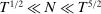 . Note that, if the PCs in the groups were observed, then testing for unit canonical correlations would be degenerate, as it involves testing for deterministic relationships between random vectors. The estimation errors of the PCs drive the asymptotic distribution of the statistic, with a nonstandard convergence rate. It might be surprising that we find an asymptotic Gaussian distribution when testing a hypothesis for a parameter at the boundary, that is, canonical correlations equal to 1. What makes the test asymptotically Gaussian is the fact that there is a re-centering of the statistic due to the sampling error in the first-step estimates of the PCs, and a CLT applies to the recentered squared estimation errors. The re-centering term involves a component of order
  and a component of order
  . One may wonder whether this Gaussian asymptotic distribution is a good approximation for the small sample distribution of the recentered and rescaled
  . In Section 6 and OA Section E, we report the results of extensive Monte Carlo simulations showing that this is the case in a setting that mimics our empirical application.
 , we need consistent estimators for the unknown scalars
  and
and  , and matrices
  and
and  in Theorem 1. To simplify the analysis, we assume at this stage that the errors
  are (i) uncorrelated across sub-panels j and individuals i, at all leads and lags, and (ii) a conditionally homoscedastic martingale difference sequence for each individual i, conditional on the factor path, that is,
 (4.4)
(4.4) (4.5)
(4.5) and
and  do not depend on time. The projection residual
  vanishes because
  , where
  , is spanned by
  . This explains why
  is null and the convergence rate is
  . Similarly,
  , so that the bias term at order
  is zero.6 Under (4.4), the bias component
  in the PC estimates is immaterial since it can be absorbed in the transformation matrix
  in (4.2). In fact, Connor and Korajczyk (1986) and Bai (2003, Theorem 4) showed that the principal component estimator is consistent even for fixed T in such a case. In Theorem 2 below, we replace
  with its large sample limit
  , matrices
  and
and  by consistent estimators. We show that the estimation error for
  in the bias adjustment is of order
  , and therefore the asymptotic distribution of the statistic is unchanged.
Theorem 2.Let  , with
  , where
  ,
,  and
and  are the loadings estimators defined in equations (3.3) and (3.4),
  with
with  , and
, and  , for
, for  . Define the test statistic:
 (4.6)
(4.6)- (i) Under the null hypothesis
 of
of  common factors, we have
  .
. - (ii) Under the alternative hypothesis
 , we have
  .
.
Proof.See Appendix B.2. □
The feasible asymptotic distribution in Theorem 2 is the basis for a one-sided test of the null hypothesis of  common factors. The rejection region for a test of the null hypothesis at asymptotic level α is
  , where
  is the α-quantile of the standard Gaussian distribution for
  . From Theorem 2 (ii), the test is consistent.
One way to implement the model selection procedure to estimate the number of common factors  proposed in Section 3.2 consists in testing sequentially the null hypothesis
  , against the alternative
  , using the test statistic
  defined in Theorem 2 for any generic number r of common factors. A “naive” procedure is initiated with
  , proceeds backwards, and is stopped at the largest integer
  such that the null
  cannot be rejected, that is,
  . Otherwise, set
  if the test rejects the null
  for all
  . This “naive” procedure is not a consistent estimator of the number of common factors. Indeed, asymptotically, a nonzero probability α of underestimating
  exists coming from the type I error of the test of
  against
  , when the true number of factors
  is strictly positive.
 , for any integer
  , is obtained allowing the asymptotic size α to go to zero as N,
  . The following Proposition 2 (proved in OA Appendix C.2) defines a consistent inference procedure for the number of common factors.
Proposition 2.Let  be a sequence of real scalars defined in the interval
  for any
  , such that (i)
  and (ii)
  for
for  . Then, under Assumptions A.1–A.9, the estimator of the number of common factors defined as

 , if
, if  for all
  , is consistent, that is,
  under
under  , for any integer
  .
.
 against
  . Condition (ii) is a lower bound on the convergence rate to zero of the asymptotic size, and is used to keep asymptotically zero probability of type II error of each step of the procedure. The conditions in Proposition 2 are satisfied, for example, for
  such that
 (4.7)
(4.7) and
and  .7
.75 Mixed-Frequency Group Factor Models
The idea to apply group factor analysis to mixed-frequency data is novel as frequency-based grouping can indeed be the basis of identification strategies and statistical inference. In this section, we explore this topic as it pertains to our empirical application. We consider a setting where both low- and high-frequency data are available. Let  be the low-frequency (LF) time units. Each time period
  is divided into M sub-periods with high-frequency (HF) dates
  , with
  . Moreover, we assume a panel data structure with a cross-section of size
  of high-frequency data and
  of low-frequency data. It will be convenient to use a double time index to differentiate low- and high-frequency data. Specifically, we let
  , for
, for  , be the high-frequency data observation i during sub-period m of low-frequency period t. Likewise, we let
  , with
  , be the observation of the ith low-frequency series at t. These observations are gathered into the
  -dimensional vectors
  , for all m, and the
  -dimensional vector
  , respectively.
 ,
,  , and
, and  , respectively. The first represents a vector of factors which affect both high- and low-frequency data (we use again superscript C for common), whereas the other two types of factors affect exclusively high (superscript H) and low (marked by L) frequency data. We denote by
  ,
,  , and
, and  the dimensions of these factors. The latent factor model with high-frequency data sampling is
 (5.1)
(5.1) and
and  , and
, and  ,
,  ,
,  , and
, and  are matrices of factor loadings. The vector
  is unobserved for each high-frequency sub-period and the measurements, denoted by
  , depend on the observation scheme, which can be either flow-sampling or stock-sampling (or some general linear scheme).
 across all m, that is,
  .8 Then, model (5.1) implies
 (5.2)
(5.2) ,
,  ,
,  , and the aggregated factors:
  ,
,  , H, L. Then we can stack the observations
  and
and  and write
 (5.3)
(5.3) and group-specific factors
  and
and  . The normalized latent common and group-specific factors
  ,
,  , satisfy the counterpart of (2.2).
The results in Sections 2, 3, and 4 can be applied for identification and inference in the mixed-frequency factor model. Using the same arguments in the mixed-frequency setting of equation (5.3), identification can be achieved for the aggregated factors  ,
,  , and
, and  , and the factor loadings
  ,
,  ,
,  , and
, and  . Consequently, the estimators and test statistics developed for the group factor model (2.1) can also be used to define estimators for the loadings matrices
  ,
,  ,
,  ,
,  , and the aggregated factor values
  ,
,  , and the test statistic for the common factor space dimension
  in equation (5.3). We denote these estimators
  ,
,  ,
,  ,
,  ,
,  , and also the infeasible and feasible test statistics
  and
and  . Once the factor loadings are identified from (5.3) and estimated, the values of the common and high-frequency factors for sub-periods
  are identifiable by cross-sectional regression of the high-frequency data on loadings
  and
and  in (5.1). More specifically, the estimators of the common and high-frequency factor values are
  ,
,  ,
,  , where
  (the asymptotic distribution of the factor estimates is provided in OA Proposition D.7). Hence,
  and
and  are obtained by regressing
  on
on  and
and  across
  , for any
  and
and  . Consequently, with flow-sampling, we can identify and estimate
  and
and  at all high-frequency sub-periods. On the other hand, only
  , that is, the within-period sum of the low-frequency factor, is identifiable by the paired panel data set consisting of
  combined with
  . This is not surprising, since we have no high-frequency observations available for the LF data.
One can consider an alternative approach to inference on the number of common factors and their estimated values. Instead of first aggregating the high-frequency data as in equation (5.3) and then applying PCA in each group, one can extract the principal components directly on the high-frequency panel (and the low-frequency panel) and then aggregate the high-frequency PCA estimates. The procedure then continues identically in both approaches. In our Monte Carlo experiments, the performances of the two approaches are found to be similar (see Section 6 and OA Section E for more details). In the empirical application, the results are almost indistinguishable (see OA Section D.11.2).
6 Monte Carlo Simulation Analysis
The objectives of the Monte Carlo simulation study are: to assess the adequacy of the asymptotic distribution of  to approximate its small sample counterpart, to evaluate the finite sample size and power properties of tests for
  based on the statistics
  and
and  , and to compare the sequential testing procedure for
  in Proposition 2, vis-à-vis the alternative procedures suggested by Chen (2012) and Wang (2012). We perform our simulations in the context of the mixed-frequency setting of Section 5 to align the analysis with the empirical application.
Section E of the OA reports a detailed description of the simulation designs and tables of results. The data generating process (DGP) is the high-frequency model (5.1) with flow-sampled LF variables. The idiosyncratic innovations are independent of the factors, serially i.i.d., and possibly weakly cross-sectionally correlated within each panel—corresponding to an approximate factor model. We consider  high-frequency sub-periods, as in our empirical application with yearly and quarterly data, and different numbers of factors across DGPs, namely,
  , and
, and  , and 5. The DGP for the vector of stacked factors
  is
is  , where
  is a common scalar AR coefficient for all the
  factors and
  . The innovations
  are i.i.d.
  , where
  is a block-matrix such that
  , for
, for  ,
,  and
and  . The scaling term ς ensures that the factor normalization in (2.2) holds for
  , while the scalar parameter ϕ generates correlation between pairs of HF and LF specific factors. Factor loadings are simulated from a multivariate zero-mean Gaussian distribution, such that the cross-sectional distribution of
  's of the regressions of observables on factors mimics the empirical application. We run 4000 simulations for each DGP, and consider
  ,
,  , T as small as the ones in our empirical applications, and progressively increase them.
All the results summarized below are qualitatively similar (1) when different values of the factor autocorrelation  are considered, namely, 0 and 0.6, (2) for different (small) levels of the weak cross-sectional correlation of the idiosyncratic errors, and (3) for different magnitudes of the pervasiveness of the factors as measured by the theoretical
  's for regressions of the simulated observables on the factors. We refer the reader to the OA for additional details.
6.1 Asymptotic Gaussian Distribution, Size, and Power Properties
First, we want to verify whether the Gaussian asymptotic distribution provides a good small sample approximation for the infeasible statistic  . Figure 1 displays the empirical distribution of
  , computed under the null of
  common factors from data simulated from a DGP with
  , and overlapped with the asymptotic
  distribution. For small sample sizes as
  , and
, and  , the empirical distribution approximates well a normal distribution with unit standard deviation, but is centered around a small positive value: the empirical mean and standard deviation are 0.16, and 1.14, respectively. Nevertheless, the left tail of this empirical distribution resembles relatively well the one of a standard Gaussian. As the sample sizes grow to
  , and
, and  , the empirical distribution of
  has empirical mean and standard deviation of 0.02 and 1.01, respectively, and almost perfectly overlaps with the asymptotic distribution. As these results are qualitatively similar for alternative DGPs and sample sizes, we conclude that our asymptotic theory provides a good approximation also in small samples.

Small sample distribution of the recentered and rescaled  statistic. The figure displays the histograms of the empirical distribution of the recentered and rescaled
  statistic computed on mixed-frequency panels of observations, for different sample sizes NH, NL, T, simulated from a DGP where kC = kH = kL = 1, all factors and idiosyncratic terms are generated from Gaussian random variables, and M = 4. The solid line corresponds to the asymptotic standard Gaussian distribution of the recentered and rescaled statistic.
The tables in OA Section E.5 display the empirical size of the tests for the null hypotheses of  or 2, common factors corresponding to nominal sizes of
  ,
,  , and
, and  . They also report the empirical power of tests for the null hypothesis of
  common factors, when the true number of common factors is
  . We observe that the asymptotic Gaussian distribution provides an overall very good approximation for the left tail of the infeasible test statistics
  under the null, even for samples as small as
  , and
, and  , corroborating the graphical evidence of Figure 1. For the vast majority of sample sizes, and simulation designs, the size distortions are in the order of 1% to maximum 3% for the designs in which
  . The size distortions for the feasible statistic
  are from 1% to 12% larger than those of the infeasible statistic when
  , and
, and  . The designs in which
  for samples as small as
  , and
, and  feature larger size distortions for smaller samples due to the fact that, by construction of the designs, the signal-to-noise ratio for each of the two common factors is halved compared with the designs in which
  . As expected, when either the sample sizes, or the signal-to-noise ratio of the common factors increase, the size distortions monotonically disappear. The power of the feasible test statistics is always equal to 1, with the exception of designs with
  , and
, and  .
.
6.2 Estimation of the Number of Common Factors
We compare the following three estimators of  : (a) the consistent sequential testing procedure of our Proposition 2, (b) a selection procedure based on the penalized information criterion of Theorem 3.7 in Chen (2012), and (c) the three-steps selection procedure proposed by Wang (2012).9 We focus on the average estimated number of common factors computed over the 4000 simulations.
We consider both the case in which the true numbers of pervasive factors  and
and  in the two panels are known, and the case where they are estimated using the
  information criterion of Bai and Ng (2002). Generally, the estimates of
  and
and  are very precise and do not affect significantly the estimation of
  . The only exceptions are the smaller samples with
  , and the DGPs with many pervasive factors in the LF panel, say
  , where the
  criterion tends to severely underestimate the values of
  , while the
  produces better estimates.10 The critical value for our selection procedure is as in equation (4.7), with
  , and
, and  .
.
For a small number—say not larger than 3—of uncorrelated specific factors, the penalized information criterion proposed in Chen (2012) yields the correct number of factors in almost all simulations for any sample size, while our selection procedure is less accurate only for sample sizes as small as  , and
, and  : the average value of
  ranges between 0.85 and 1 for
  . The average value of
  for our selection procedure approaches quickly the true value
  as the sample sizes increase.
The procedure of Chen (2012) overestimates  when the correlation ϕ among the specific factors increases from 0 to 0.7, and 0.95. The overestimation is much less severe for our sequential test procedure, also in larger samples, which also features a faster improvement in performance as the sample sizes increase. We observe a monotonic decrease in the precision across all the estimators when the number of specific factors becomes as large as 5; nevertheless, the deterioration in performance is less pronounced for our procedure. Finally, the consistent three-steps selection procedure of Wang (2012) performs similarly to the one of Chen (2012) in DGPs with a small number of uncorrelated specific factors. However, as either ϕ or the numbers of specific factors increase, this procedure largely overestimates
  and becomes the worst among the three considered.
7 Empirical Application
Recent public policy debates argue that manufacturing has been declining in the United States and most jobs have migrated overseas to lower wage countries. The share of the Industrial Production (IP) sector declined from more than 25% to roughly 18% during our sample period 1977–2011. However, the fact that its size shrank does not necessarily exclude the possibility that the IP sector still is a key factor of total U.S. output. When studying the role of the IP sector, we face a conundrum. On the one hand, we have 117 sectors that make up aggregate IP. These data are published monthly, and therefore cover a rich time series and cross-section. On the other hand, contrary to IP, we do not have monthly or quarterly data regarding the cross-section of U.S. output across non-IP sectors, but we do so on an annual basis. Using the class of mixed-frequency group factor models proposed in Section 5, the objective of the empirical application is to shed light on the key question of interest, namely, whether, despite the shrinking size of IP sectors, the factors related to IP are still dominant determinants of U.S. output fluctuations.
7.1 Data Description
For the IP sectors, we use the same 117 IP sectoral growth rates indices sampled at quarterly frequency from 1977.Q1 to 2011.Q4, as in Foerster, Sarte, and Watson (2011) for comparison.11 The data for all the remaining non-IP sectors consist of the annual growth rates of real GDP for the following 42 sectors: 35 Services, Construction, Farms, Forestry-fishing, and related activities, General government (federal), Government enterprises (federal), General government (state and local), and Government enterprises (state and local). These LF data are published by the Bureau of Economic Analysis (BEA).12 Hence we consider the panel of these yearly GDP sectoral and the quarterly IP data given that one of the objectives of this application is to study the comovements among these different sectors. A description of the practical implementation of our procedure appears in OA Section D.9.13
7.2 Common, Low-, and High-Frequency Factors
We assume that our data set follows the factor structure for flow-sampling as in equation (5.2), with  and
and  corresponding to the 117 quarterly IP series and the 42 annual GDP non-IP sector data series, respectively, for the period 1977.Q1–2011.Q4. We exclude the annual series related to IP sectors from the annual GDP panel in order to avoid double counting. Let
  be the
  panel of the yearly observations of the IP indices growth rates computed as the sum of the quarterly growth rates
  ,
,  , for year t, and let
  be the
  panel of the yearly growth rates of the non-IP indices. Let also
  be the
  panel of quarterly IP indices growth rates.
We start by selecting the number of factors in each sub-panel, which are of dimensions  for
for  and
and  and
and  for
for  . We use the
  and
and  information criteria of Bai and Ng (2002), following the empirical literature. For the panels of IP growth rate at quarterly (
 ) and annual (
 ) frequencies,
  selects two factors for each panel, whereas the more strict
  criterion selects one factor for
  and two factors for
  . For the annual GDP (non-IP) sectors panel, both
  and
and  select a single factor.14 Our results corroborate the evidence in Foerster, Sarte, and Watson (2011), suggesting that there are either one or two pervasive factors in the quarterly IP growth data. While the
  and
and  choose factors in an unconditional setup, we are also interested in the explanatory power of these factors in a conditional setup. Hence the empirical analysis proceeds with two factors for each panel,
  , in order to avoid potentially omitted factors/variables in explaining economic activity growth and subsequently re-assess the conditional significance of factors using the BIC criterion.15
In order to select the number of common and frequency-specific factors, we follow our proposed procedure in Proposition 2. The estimated canonical correlations of the first two PC's estimated in each sub-panel  and
and  are used to compute the value of the feasible standardized test statistic
  in (4.6) and Theorem 2, for testing the null hypotheses of
  and
and  common factors.16 The first canonical correlation is
  , while the second one is
  . These results are consistent with the presence of one common factor in each of the two mixed-frequency data sets considered, as represented by hypothesis
  in Section 3.2. The values of the statistics are
  and
and  for the null hypotheses of
  and
and  common factors, respectively. The test rejects the null hypothesis of the presence of two common factors (
 ), for significance levels as small as 0.05%, while we cannot reject the null of one common factor at the 5% significance level. Our selection procedure detailed in Proposition 2 with critical level as in (4.7) with
  and
and  , produces the estimate
  . Hence, we select a model with
  .
.
In Figure 2, Panel (a) plots the IP and GDP growth rates during the period 1977–2011 and the remaining Panels (b)–(d) present the estimated factor paths from the panels of 42 GDP sectors and 117 IP indices for the common, the HF-specific, and the LF-specific factors, respectively. All factors are standardized to have zero mean and unit variance in the sample and their sign is chosen so that the majority of the associated loadings are positive. A visual inspection of the plots reveals that the common factor in Panel (b) resembles the IP index in Panel (a), with a large decline corresponding to the Great Recession following the financial crisis of 2007–2008 and the positive spike associated to the recent economic recovery. On the other hand, the LF-specific factor displayed in Panel (d) features a less dramatic fall during the Great Recession, and actually features a positive spike in 2008, followed by large negative values in the following years. This constitutes preliminary evidence suggesting that some non-IP sectors could feature different responses to the recent financial crisis.
The relationship of factors with the sectoral GDP and IP growth series, in a regression context, reveals additional information about the conditional correlations of the factors with specific economic activity growth sectors. This in turn can help us shed light on which IP and non-IP series are driving the factors. We start with a disaggregated analysis, and examine the relative importance of the common and frequency-specific factors in explaining the variability across all sectoral growth rates. For each sector in the panel, we regress the GDP or IP index growth rates on (i) the common factor only, (ii) the specific factor only, for non-IP and IP series, respectively, and (iii) both common and specific factors. In Table I, we report the quantiles of the empirical distribution of the adjusted  (denoted
  ) of these regressions. In addition, we report the percentage value of the times the BIC (denoted by %BIC) selects, among the aforementioned three regression models (i)–(iii), the alternative factor conditional information set (common and/or frequency-specific), for each sectoral index in the cross-section.17
 and Percentage Values of BIC of the Regressions With Common and/or Frequency-Specific Factors From Economic Activity Indices Growth Ratesa
|
|
||||||
|---|---|---|---|---|---|---|
|
Factors |
10% |
25% |
50% |
75% |
90% |
% BIC |
|
Observables: Gross Domestic Product, 1977–2011 |
||||||
|
common |
−2.2 |
−0.5 |
11.5 |
28.9 |
42.9 |
38.1 |
|
common, LF-specific |
0.1 |
9.2 |
25.4 |
34.5 |
60.3 |
28.6 |
|
LF-specific |
−2.8 |
−2.3 |
5.7 |
15.7 |
22.4 |
33.3 |
|
Observables: IP, 1977.Q1–2011.Q4 |
||||||
|
common |
0.3 |
4.8 |
20.3 |
36.0 |
60.0 |
42.7 |
|
common, HF-specific |
1.1 |
6.8 |
28.7 |
45.3 |
63.4 |
48.7 |
|
HF-specific |
−0.7 |
−0.1 |
3.0 |
11.2 |
23.5 |
8.5 |
 : Quantiles
- a
The regressions in the first three lines involve the growth rates of the 42 non-IP sectors as dependent variables, while those in the last three lines involve the growth rates of the 117 IP indices as dependent variables. The explanatory variables are factors estimated from the same indices using a mixed-frequency factor model with
 . Reported are the adjusted
  of the regressions on common and/or frequency-specific factors for different quantiles of the cross-section. The last column reports the percentage values that the BIC chooses the specific factor type regression model.
From the first three lines in Table I, we observe that adding the LF-specific factor to the common factor regressions for the non-IP indices yields an increment of the median  around 14% (going from 11.5% to 25.4%) and the 90% quantile of
  increases by 17%. Adjusting for the number of the variables in the factor regression models, the BIC favors the model with both the common and the LF-specific factors in explaining the GDP growth rate in 29% of the sectors, whereas the model with the common factor alone is selected in about 38% of the series. When the high-frequency-specific factor is added to the common factor, it contributes an increment of around 8% in the median
  for the IP sectors. The 49% BIC value provides strong evidence that both the common and high-frequency factors explain the IP sectoral growth rate. Overall, the results in Table I show that the common factor turns out to be pervasive for most of the IP and non-IP sectors alike as demonstrated by both the relative
  vis-à-vis those with just the frequency-specific factor.
In order to investigate which sectors drive the variation of our estimated factors and provide an economic interpretation to our factors, we list in Table II the highest and lowest ten GDP non-IP sectors in terms of  when regressed on the common factor only (in Panel A), and both the common and LF-specific factors (in Panel B). We also report the top and bottom ten ranked GDP non-IP sectors with the highest and lowest absolute increments in
  when the LF-specific factor is added to the common one (in Panel C).18
 a
a|
Panel A. Regressor: common factor |
Panel B. Regressors: common and LF-specific factors |
Panel C. Increment in adj. |
|||
|---|---|---|---|---|---|
|
Sector |
|
Sector |
|
Sector |
|
|
Ten sectors with largest |
Ten sectors with largest |
Ten sectors with largest |
|||
|
Truck transportation |
63.10 |
Misc. prof., scient., & tech. serv. |
66.67 |
Misc. prof., scient., & tech. serv. |
49.69 |
|
Accommodation |
62.43 |
Admin. & support services |
62.63 |
Gov. enterprises (state & local) |
34.69 |
|
Construction |
44.05 |
Truck transportation |
62.51 |
Rental & leasing serv. |
29.52 |
|
Other transp. & support activ. |
43.31 |
Accommodation |
61.48 |
General gov. (state & local) |
24.90 |
|
Administrative & support services |
42.69 |
Construction |
59.75 |
Legal services |
24.32 |
|
Other services, except gov. |
42.53 |
Warehousing & storage |
52.53 |
Motion picture & sound rec. |
22.77 |
|
Warehousing & storage |
40.95 |
Gov. enterprises (state & local) |
45.78 |
Fed. Res. banks, credit interm.. |
20.31 |
|
Air transportation |
31.58 |
Other services, except gov. |
41.75 |
Administrative & support services |
19.95 |
|
Retail trade |
30.70 |
Other transportation & support act. |
41.71 |
Social assistance |
19.91 |
|
Amusem., gambling, & recr. ind. |
29.17 |
gov. enterprises (federal) |
37.78 |
Real estate |
18.14 |
|
Ten sectors with smallest |
Ten sectors with smallest |
Ten sectors with smallest |
|||
|
Funds, trusts, & other finan. vehicles |
−1.23 |
Ambulatory health care services |
7.76 |
Accommodation |
−0.96 |
|
Motion picture & sound record. ind. |
−1.68 |
Management of comp. & enterpr. |
7.52 |
Rail transportation |
−1.16 |
|
Pipeline transportation |
−1.74 |
Funds, trusts, & other fin. vehicles |
6.15 |
Other transportation & support act. |
−1.59 |
|
Information & data processing services |
−1.84 |
Information & data processing services |
1.96 |
Air transportation |
−1.77 |
|
Transit & ground passenger transp. |
−2.05 |
Educational services |
1.35 |
Retail trade |
−2.15 |
|
General gov. (state & local) |
−2.12 |
Insurance carriers & related activities |
0.36 |
Amusements, gambling |
−2.15 |
|
Forestry, fishing & related activities |
−2.33 |
Water transportation |
−0.64 |
Educational services |
−2.62 |
|
Water transportation |
−2.94 |
Farms |
−1.87 |
Farms |
−2.80 |
|
Securities, commodity contr., & investm. |
−2.99 |
Forestry, fishing |
−5.31 |
Forestry, fishing |
−2.98 |
|
Insurance carriers |
−3.03 |
Securities, commodity contr. |
−5.99 |
Securities, commodity contr. |
−3.00 |
 in Panels A and B


- a
The adjusted
 , denoted
  , are reported for the restricted MIDAS regressions of the growth rates of 42 GDP non-IP sectoral indices on the estimated factors. Regressions in Panel A involve a LF explained variable and the estimated common factor. Regressions in Panel B involve a LF explained variable and both the common and LF-specific factors. In Panel C, we report the difference in
  (denoted as
  ) between the regressions in Panel B and regressions in Panel A.
From Panel A, we first note that the common factor alone explains most of the variability of service sectors with direct economic links to IP sectors like Truck transportation, Administration & Support Services, and Warehousing, with an  ranging from 63% to 43%, as well as Accommodation with
  of 63%. This indicates that the common factor is driven by service sectors related to IP and could thereby be interpreted as an IP factor, as already noted on Figure 2. On the other hand, the common factor turns out to be completely unrelated to most of the Financial, Insurance, and Information services sectors. Turning to Panel C of Table II, which reports the difference in
  between the regressions in Panels A and B, we note that the LF-specific factor explains more than 20% of the variability of output for very heterogeneous services sectors as well as Government (state and local).19 Interpreting these results, we conclude that the LF-specific factor is completely unrelated to service sectors which depend almost exclusively on IP output (e.g., transportation, retail trade), and is a common factor driving the comovement of other non-IP service sectors, such as Professional scientific and technical services, Government, legal services.

Sample paths of IP and GDP growth rates and the estimated factors, 1977–2011. Panel (a) displays the dashed/circled line which corresponds to the quarterly growth rates of the aggregate IP index for sample period 1977.Q1–2011.Q4, and the solid line which represents the annual growth rates of GDP for the entire U.S. economy. Panel (b) displays the path of the estimated common factor. Panel (c) displays that of the HF-specific factor and Panel (d) that of the LF-specific factor. The factors are estimated from the panels of 42 annual non-IP GDP sectoral series and 117 quarterly IP indices using a mixed-frequency group factor model with kC = kH = kL = 1.
In Table II, we highlight further differences in the dynamics of output growth between the two sub-sectors of the financial services industry which are particularly revealing, Securities and Credit intermediation, extensively studied by Greenwood and Scharfstein (2013). We find that the sub-sectors Funds, trusts, and other financial vehicles as well as Securities, commodity contracts, and investments, are unrelated to both the common and LF-specific factors, indicating that their output growth is uncorrelated with the common component of real output growth and across the other sectors that correlate with the U.S. economic activity. In contrast, the Credit intermediation industry comoves with the other IP and non-IP sectors (see Tables D.24 and D.25 in the OA).
Up to this point, we examined the explanatory power of the factors for sectoral output indices. For non-IP GDP, these indices correspond to the finest level of disaggregation of output growth by sector. In Table III, we report the results of regressions with aggregated indices instead. In particular, we regress the output of each aggregate index either on the estimated (a) common factor, (b) frequency-specific, or (c) both aforementioned factors, and report the corresponding  of these regressions in the first three columns. The last column in Table III reports the model favored by the BIC among the three regression specifications. It is important to note that now we also include the GDP Manufacturing aggregate index which is not used in the estimation of the factors. Panel A in Table III shows that the common factor explains around 89% of the variability in the aggregate IP growth index, confirming that this factor can be interpreted as an IP factor during the period 1977–2011. This is further corroborated in Panel B where we obtain an
  of 82% in the regression of the GDP Manufacturing Index on the common factor alone. As most of the sectors included in the IP index are Manufacturing sectors, this result is not surprising. Yet, it is still worth noting because, as remarked earlier, the GDP data on Manufacturing have not been used in the factor estimation, in order to avoid double-counting these sectors in our mixed-frequency sectoral panel.20
|
Panel A Quarterly observations, 1977.Q1–2011.Q4 |
|||||
|
(1) |
(2) |
(3) |
(3)-(1) |
||
|
Sector |
|
|
|
BIC |
|
|
Industrial Production |
89.06 |
5.02 |
90.26 |
1.20 |
CH |
|
Panel B Yearly observations, 1977–2011 |
|||||
|
(1) |
(2) |
(3) |
(3)-(1) |
||
|
Sector |
|
|
|
||
|
GDP |
60.54 |
8.59 |
74.21 |
13.67 |
CL |
|
GDP—Manufacturing |
81.88 |
−3.03 |
81.53 |
−0.35 |
C |
|
GDP—Agriculture, forestry, fishing, & hunting |
1.43 |
−2.52 |
−1.26 |
−2.69 |
C |
|
GDP—Construction |
44.05 |
11.22 |
59.75 |
15.70 |
CL |
|
GDP—Wholesale trade |
20.35 |
7.90 |
30.83 |
10.48 |
CL |
|
GDP—Retail trade |
30.70 |
−2.86 |
28.56 |
−2.15 |
C |
|
GDP—Transportation & warehousing |
62.14 |
−2.95 |
60.97 |
−1.17 |
C |
|
GDP—Information |
12.14 |
22.28 |
37.57 |
25.43 |
CL |
|
GDP—Finance, insurance, real estate, rental, & leasing |
−1.42 |
21.22 |
21.11 |
22.53 |
L |
|
GDP—Professional and business services |
30.02 |
30.21 |
65.61 |
35.59 |
CL |
|
GDP—Educational serv., health care, and social assistance |
−1.38 |
18.38 |
18.18 |
19.56 |
L |
|
GDP—Arts, entertainment, recreation, accommodation, & food serv. |
53.51 |
−2.23 |
53.70 |
0.18 |
C |
|
GDP—Government |
−2.12 |
22.37 |
20.47 |
22.59 |
L |


- a
The adjusted
 , denoted
  , of the regression of growth rates of the aggregate IP index and selected aggregated GDP output indices on the common factor (column
  ), the specific HF and LF factors only (columns
  and
and  ), and the common and frequency-specific factors together (column (3)) are reported. The fourth column displays the difference between the values in the third and first columns. The last column reports the choice of the BIC across the regression models with the common factor, or the frequency-specific factor, or both factors (C denotes the common factor, H denotes the high-frequency factor, and L denotes the low-frequency factor and corresponding factor combinations (CL and CH) in the regression models). The factors are estimated from the panel of 42 GDP non-IP sectors and 117 IP indices using a mixed-frequency factor model with
  .
.
Looking at the aggregate GDP index, we first note that even if the weight of IP sectors in the aggregate GDP index has always been below 30%, still 61% of its total variability can be explained exclusively by the common factor which—as shown in Panel B—is primarily an IP factor. This implies that there must be substantial comovement between IP and some important service sectors. Moreover, it appears from the first line in Panel B that a relevant part of the variability of the aggregate GDP index not due to the common factor is explained by the LF-specific factor (since the  increases by about 14% from 60.5% to 74.2%). This indicates that significant comovements are present among the most important sectors of the U.S. economy which are not related to manufacturing. Indeed, Panel B indicates that some services sectors such as Professional and Business Services and Information, as well as other sectors such as Wholesale trade and Construction, load significantly on both the common and the LF-specific factor, while some other sectors like Finance and Government load exclusively on the LF-specific factor.21
The BIC in Table III, Panel B, favors the regression model with both the common and low-frequency factors, among the three factor regression specifications for the U.S. GDP growth rate, while the low-frequency factor alone yields a low  of 9%. Similarly, although the HF-specific factor in Panel A seems to be relatively less important in explaining the aggregate IP index (as the
  increases by only 1% when it is added as a regressor to the common factor regression model for the IP growth rate), the BIC suggests that both the common and HF factors are important.22 Overall, the small
  could suggest that the HF-specific factor is pervasive only for a subgroup of IP sectors which have relatively low weights in the index, meaning that their aggregate output is a negligible part of the output of the entire IP sector and, consequently, also the entire U.S. economy. These results corroborate the findings of Foerster, Sarte, and Watson (2011), who claimed that the main results of their paper are qualitatively the same when considering either one or two common factors extracted from the same 117 IP indices of our study. It is worth emphasizing that the common factor explains the dominant 89% of the variability of the total IP growth and 61% of the GDP growth.
Given that our sample period covers the Great Moderation, characterized by a reduction in the volatility of business-cycle fluctuations starting in the mid-1980s, we revisit this analysis for different sub-samples. The details can be found in OA Section D.11.4, while we discuss here briefly the main results. We find a deterioration of the overall fit of approximate factor models during the Great Moderation period starting in 1984 and ending in 2007—a finding also reported by Foerster, Sarte, and Watson (2011)—where our common factor plays a relatively less significant role during that period. Interestingly, when the financial crisis is added to the Great Moderation (sample 1984–2011), we find patterns closer to the full sample results presented above. The other findings, that is, the exposure of the various sub-indices, appear to be similar in sub-samples and in the full sample.
8 Conclusions
We present a general framework for group factor models and develop a unified asymptotic theory for the identification of common and group factors, for the determination of the number of common and specific factors, for the estimation of loadings and factor values via principal component analysis and canonical correlation analysis in a setting with large-dimensional data sets, using asymptotic expansions both in the cross-sections and in time-series dimensions. Of special interest is the group factor mixed-frequency model for which the data panels of different/mixed frequencies allow not only for a natural grouping in extracting factors but also a framework which has the advantage of identifying and estimating factors which are common across frequencies as well as frequency-specific.
Our theoretical contributions, in particular Theorems 1 and 2, are of interest beyond (mixed-frequency) group factor models. Inference regarding the rank of an unknown, real-valued matrix is an important and well-studied problem.23 For indefinite matrix estimators, there is a well-developed framework; see Donald, Fortuna, and Pipiras (2007). The case of semi-definite matrix estimators still poses many challenges, however, as discussed by Bai and Ng (2007) and more recently in Donald, Fortuna, and Pipiras (2010) who argued that the tests suggested in the literature are not suitable. In fact, when the rank of a generic (positive) semi-definite matrix, say V, needs to be estimated using a semi-definite estimator, say  , the asymptotic variance-covariance matrix of this estimator—denoted as
  —is necessarily singular, as shown in Donald, Fortuna, and Pipiras (2007). Therefore, standard rank tests cannot be applied as they assume that the matrix
  is full rank. In addition, our results in Section 4 provide the guidance to the construction of the asymptotic distribution of the (sum of the) eigenvalues of a semi-definite matrix, and develop a sequential testing procedure for determining the rank of the matrix itself. This test, for example, would enable us to determine the number of latent dynamic factors in large panels of data, without having to estimate them, a problem tackled by Bai and Ng (2007). In their paper, first a number—say r—of static factors should be estimated by PCA from a large panel. Differently from their methodology, and also differently from the solution proposed by Amengual and Watson (2007), we can directly test the rank—say
  —of the residual covariance (or correlation matrix) of a VAR model estimated on the factors themselves. Furthermore, our methods can be used to develop a new test for the question posed by Pelger (2019) as to whether the factor spaces of statistical and economic factors are equal.
There is a plethora of applications to which our theoretical analysis applies. We selected a specific example based on the work of Foerster, Sarte, and Watson (2011) who analyzed the dynamics of comovements across 117 IP quarterly sectors using factor models. We revisit part of their analysis and incorporate the rest—and most dominant part—of the U.S. economy, namely, the non-IP sectors whose growth rate we only observe annually. We find evidence for a single common factor among IP and non-IP sectors which explains 89% of the aggregate IP index and 61% of the aggregate GDP index.
Despite the generality of our analysis, we can think of many possible extensions, such as models with loadings which change across sub-periods, that is, periodic loadings, or loadings which vary stochastically or feature structural breaks. Moreover, we could consider the problem of specification and estimation of a joint dynamic model for the common and frequency-specific factors extracted with our methodology (see Ghysels (2016) and the references therein for structural Vector Autoregressive (VAR) models with mixed-frequency sampling). Further, in the interest of conciseness, we have focused our analysis on models with two sampling frequencies, leading to group factor models with two groups. Results could be extended to cover the cases with more than two groups, and therefore more than two sampling frequencies. All these extensions are left for future research.
 ,
,  , and
, and  . Proposition D.1 is implied by Proposition 1 in Wang (2012).
 principal components of the pooled data is inconsistent due to the correlation in the residuals terms arising from the group-specific factors, and (2) the combined data may not give the common factors because the common factors may not even be the leading factors in the combined data.
 and
and  requires thresholding of estimated cross-sectional covariances and/or HAC-type estimators. If the errors are conditionally heteroscedastic, we need consistent estimators of
  and
and  as well.
 and
and  , which yields, for example,
  close to 0.05 for
  and
and  , that are the smallest cross-sectional size and the low-frequency time-series dimension in our data set. In the Monte Carlo study, we find a good performance of the selection procedure with this choice.
 , which is a special case of the one suggested by Wang (2012): (i) estimate the numbers
  and
and  of pervasive factors in each panel separately, (ii) estimate the number R of pervasive factors in the stacked panel of flow-sampled HF and LF data, (iii) estimate
  as
as  . We use the
  criteria of Bai (2003) to estimate the number of factors in the first two steps.
 ,
,  , and also R, using the ER and GR ratios of Ahn and Horenstein (2013), and noted that they perform similarly or worse than the
  criterion. Alternative estimators, such as the one proposed by Onatski (2010), could also be considered.
 as maximum number of factors when computing
  and
and  .
.
 corresponding to the first and second lines (resp., fourth and fifth lines) of Table I are represented in the histograms available in OA, Figures D.11(a) and (b) (resp., (c) and (d)).
 of the regression of all GDP indices on the HF factor only, and all the three factors together.
 for some
  , where
  , where
  , and similarly for
  .
.
 , then
  is not negligible with respect to
  . Similarly, if
  , then
  is not negligible with respect to
  . In those cases, we need a more accurate asymptotic expansion.
 , uniformly in
  and
and  , where
  for some
  .
.
Appendix
We use the following notation. Let  denote the Frobenius norm of matrix A. We denote by
  the
the  -norm of random matrix Z, for
  . We denote by
  convergence in distribution. For a sigma-field
  , we denote by
  (
( -stably) the stable convergence on
  of a sequence of random vectors, that is,
  as
as  , for any Borel set A with
  , where ∂A is the boundary of set A, and any measurable set
  (see, e.g., Renyi (1963), Aldous and Eagleson (1963), Hall and Heyde (1980), Kuersteiner and Prucha (2013)). In particular, for a symmetric positive-definite random matrix Ω measurable with respect to
  , by
, by  (
( -stably) we mean
  (
( -stably), where
  is independent of
  .
.
Appendix A: Assumptions
We make the following assumptions:
Assumption A.1.We have  such that the conditions in (4.1) hold.
Assumption A.2.The unobservable factor process  satisfies the normalization restrictions in (2.2), with
  positive-definite.
Assumption A.3.The loadings matrix  is such that
  , where
  is a positive-definite
  matrix with distinct eigenvalues and
  , for
, for  .
.
Assumption A.4.The error terms  and the factors
  are such that, for
  and all
  : (a)
: (a)  and
and  , a.s., where
  , (b)
, (b)  and
and  , for a constant
  , where
  is defined in Assumption A.5 (b).
Assumption A.5.Define the variables  and
and  , indexed by
  , where
  , for
, for  . (a) For any
  and
and  we have

 , where the asymptotic variance matrix is

 , for any
  .
.Moreover, for all  and
and  , we have (b)
  , a.s., and (c)
  , for constants
  and
and  .
.
Assumption A.6.(a) The triangular array processes  and
and  are strong mixing of size
  , uniformly in
  .24 Moreover, (b)
  , as
, as  , uniformly in
  , and (c)
  , as
, as  , uniformly in
  , for
, for  , where
  and
and  .
.
Assumption A.7.For  : (a)
: (a)  ,
,  , for any
  and a constant M, where
  ; (b)
; (b)  ,
,  ,
,  , where
  ; (c)
; (c)  and
and  , where
  and
and  , where
  .
.
Assumption A.8.For  : (a)
: (a)  , for large δ; (b)
  , for all
  ; (c)
; (c)  , for all
  and
and  , where either
  , or
, or  , or
, or  ; (d)
; (d)  , for all
  ; where
  are constants, and
  .
.
Assumption A.9.The error terms are such that: (a)  , if either
  , or
, or  , (b)
, (b)  , (c)
, (c)  , say, where
  , for all
  .
.
 is necessary for our model to have exactly
  pervasive factors. It holds if, and only if, the eigenvalues of matrix
  are smaller than 1 in modulus. The zero restrictions on the matrix
  in (2.2), corresponding to the orthogonality of the common and group-specific factors, as well as the identity diagonal blocks, are identification conditions. Assumption A.3 concerns the empirical cross-sectional second-order moment matrix of the loadings in each group
  . It implies that matrix
  has full column-rank, for
  large enough,
  . Positive-definiteness of matrix
  , for
, for  , is also necessary for the existence of exactly
  pervasive factors. Note that we consider non-random loadings to simplify the assumptions and proofs. If the loadings were random, stochastic convergence could be obtained with a DGP for the loadings which satisfies the conditions of the LLN for weakly dependent data. Assumptions A.2 and A.3 are similar to conditions used in the large-scale factor model literature (see Assumptions A and B in Bai and Ng (2002, 2006), Bai (2003), among others).
Assumption A.4 requires the existence of higher-order moments for the factors and the error terms, similarly as, for example, in Assumptions A and C.1 in Bai and Ng (2002) and Bai (2003).
Assumption A.5 constrains the amount of admissible cross-sectional dependence of the error terms across different individuals, in the spirit of the framework—introduced by Chamberlain and Rothschild (1983)—of weak cross-sectional dependence characterizing “approximate factor models.” No distributional assumption is made on the idiosyncratic terms. Assumption A.5 (a) states that the cross-sectional averages of the error terms scaled by factor loadings satisfy a CLT. It corresponds to Assumption F.3 in Bai (2003). We adopt stable convergence on the sigma-field  to allow for the asymptotic variance-covariance matrix
  to possibly depend on common factors. That would occur, for example, if there are common components in the conditional volatility processes of the idiosyncratic errors. Assumption F.3 in Bai (2003) applies if the trivial filtration is replaced for
  . Assumption A.5 (b) concerns higher-order conditional moments of the scaled cross-sectional average of error terms. A sufficient condition for Assumption A.5 (b) with
  is
is  and
and  , a.s., for all
  and
and  . For
. For  , it corresponds to Assumption C.3 in Bai (2003). Assumption A.5 (c) concerns the fourth-order moment of cross-sectional averages of squared error terms and corresponds to Assumption C.5 in Bai (2003).
Assumption A.6 allows for weak serial dependence in error terms and factor processes. Specifically, Assumption A.6 (a) is a strong mixing condition, where (minus) the mixing size is inversely related to the moment order r introduced in Assumptions A.4 and A.5. We rely on this specific concept of time-series dependence because we use a CLT for data that are near-epoch dependent (NED) on mixing processes (see, e.g., Davidson (1994)), to show the asymptotic Gaussian distribution of the test statistic in Theorem 1. We deploy this specific version of the CLT for dependent data as it allows us to cope with the rather complex nature of the leading term in the asymptotic expansion of the test statistic, that involves the time-series average of the square of a cross-sectional average of scaled errors (instead of an average of averages as in the asymptotic expansion of factor estimates). We use Assumptions A.3, A.4, A.5 (a)–(b), and A.6 to check the conditions of the CLT in Section B.1.6 (i). Assumptions A.6 (b) and (c) require that certain quantities are well-approximated by their projection on a finite number of components of a mixing process to apply the NED property.
Assumption A.7 consists of additional restrictions on the weak cross-sectional and time-series dependence of the error and factor processes, which are used to prove the asymptotic expansions for the PCA estimates of the pervasive factors in the two groups in Proposition 3 in Section B.1.1. Specifically, Assumption A.7 (a) concerns cross-sectional averages of cross-products of error terms at different dates. It requires both that these cross-sectional averages are close to the corresponding population covariances in the large sample limit, and that the latter covariances decay with the time lag in a summable way. Assumptions A.7 (b) and (c) provide bounds on terms involving processes  ,
,  , and
, and  , that consist of averages of products of error terms at different dates. We elaborate on the conditions of Assumption A.7 in OA Section D.7 to show that they hold under weak primitive assumptions.
Assumptions A.5, A.6, and A.7 yield conditions of weak cross-sectional and time-series dependence to control terms such as those in Assumptions C, D, E, and F.1–F.3 in Bai (2003). They could be substituted, at the expense of more elaborated proofs, by other weak dependence assumptions for factors and idiosyncratic errors.
Assumption A.8 is used to get bounds on the remainder terms in the asymptotic expansions of estimated factors and loadings in Proposition D.4 uniformly across i and t. These bounds are used to control the estimation error for the re-centering and re-scaling terms of the feasible test statistic in Theorem 2. Specifically, Assumption A.8 (a) is a tail condition on the factor stationary distribution, Assumption A.8 (b) constrains the amount of cross-sectional dependence of the error terms, while Assumption A.8(d) is a uniform bound on true factor loadings. In Assumption A.8 (c), we require that time-series averages of certain zero-mean processes involving error terms and factors satisfy a large deviation bound. Such a large deviation bound is implied by tail conditions plus restrictions on serial dependence like strong mixing (see, e.g., Theorems 3.1 and 3.2 in Bosq (1998)).
Assumption A.9 simplifies the derivation of the feasible asymptotic distribution of the statistic in Theorem 2. This condition excludes correlation of the error terms across individuals and time (conditional on the factors), as well as conditional heteroscedasticity, and implies a “strict factor model” for each group. In that sense, it is more restrictive than Assumptions A.5, A.6, A.7, and A.8 (b)–(c). Moreover, under Assumption A.9, the matrix  in Assumption A.5 (a) simplifies to
  , while
  if either
  , or
, or  . We note that Assumption A.9 simplifies substantially the proof of Theorem 2, but is not needed in the proofs of Theorem 1 and Propositions D.4 through D.7.
Appendix B: Proofs
B.1 Proof of Theorem 1
The proof of Theorem 1 is structured as follows. We start by deriving an asymptotic expansion for the estimates of the pervasive factors extracted by PCA in each group (Section B.1.1). This result yields an asymptotic expansion for the sample canonical correlation matrix  (Section B.1.2), and, in turn, it is used to obtain the asymptotic expansions of the eigenvalues and eigenvectors of matrix
  by perturbation methods (Sections B.1.3 and B.1.4). This yields the asymptotic expansions of the canonical correlations and of the test statistic
  (Section B.1.5). Finally, the asymptotic Gaussian distribution of the test statistic follows by applying a suitable CLT for dependent triangular arrays (Section B.1.6). The proofs of Proposition 3 and technical Lemmas B.1–B.9 are provided in OA Section C.
B.1.1 Asymptotic Expansion of the Factor Estimates 
Proposition 3.Under Assumptions A.1–A.4, A.5 (b), (c), A.6 (a), and A.7, we have
 (B.1)
(B.1) ,
,  , where
  ,
,  ,
,  ,
,  , and terms
  are such that
  and
and  as
as  , and the matrix
  converges in probability to a nonstochastic orthogonal
  matrix, for
  .
.
B.1.2 Asymptotic Expansion of Matrix 
 and
and  (see, e.g., Anderson (2003)). Therefore, without loss of generality, for the asymptotic analysis of the test statistic
  , we can set
  ,
,  , in expansion (B.1). We get
 (B.2)
(B.2) (B.3)
(B.3) . From the definition of matrix
  in (3.1), and by using (B.2) and
  , we get
 (B.4)
(B.4) in Proposition 3, in the next lemma we derive an upper bound for terms
  ,
,  .
.Let us now expand matrix
 , for
, for  , where
  .
. at second order in the
  . The reason for going beyond the first order is the following. It turns out that the first-order contribution of the
  to the statistic of interest involves leading terms of stochastic orders
  and
and  (see Lemma B.5 below). The second-order remainder term is
  , and
, and  is not negligible with respect to
  , when either T is too small compared to N, or N is too small compared to T. In order to get validity of our results for more general conditions on the relative growth rate of N and T such as in Assumption A.1, we consider a second-order expansion. By using
  for
for  , from (B.4) we get the next lemma.
Lemma B.2.Under Assumptions A.1–A.4, A.5 (b)–(c), A.6 (a), and A.7, the second-order asymptotic expansion of matrix  is
is
 (B.5)
(B.5) and
and  , with
  ,
,
 (B.6)
(B.6) (B.7)
(B.7) .
.
 as the sum of the sample canonical correlation matrix
  computed with the true factor values, the estimation error term
  that consists of first-order and second-order components
  and
and  , and the third-order remainder term
  .
.
B.1.3 Matrix  and Its Eigenvalues and Eigenvectors
 and its eigenvalues, that are
  , that is, the squared sample canonical correlations of vectors
  and
and  , under the null hypothesis of
  common factors among the two groups of observables. Since the vectors
  and
and  have a common component of dimension
  , we know that
  a.s. Using the notation

 , with
  , in (B.3) in block form as

Lemma B.3.The matrix  is such that

 and
and  for
for  .
.
 is the sample canonical correlation matrix for the residuals of the sample orthogonal projections of
  and
and  onto
onto  . From Lemma B.3, the
  largest eigenvalues of matrix
  are
are  , while the remaining
  eigenvalues are the eigenvalues of matrix
  and are such that
  , a.s. Let us define
 (B.8)
(B.8) unit eigenvalues of
  are spanned by the columns of matrix
  . The columns of matrices
  and
and  span the space
  .
.B.1.4 Eigenvalues and Eigenvectors of Matrix  Obtained by Perturbation Methods
 canonical correlations are such that
  , with
  , are the
  largest eigenvalues of matrix
  . We now derive their asymptotic expansion under the null hypothesis
  using perturbations arguments applied to equation (B.5). Let
  be a
be a  matrix whose columns are eigenvectors of matrix
  associated with the eigenvalues
  , with
  . We have
 (B.9)
(B.9) is the
  diagonal matrix containing the
  largest eigenvalues of
  . We know from the previous subsection that the eigenspace associated with the largest eigenvalue of
  (equal to 1) has dimension
  and is spanned by the columns of matrix
  . Since the columns of
  and
and  span
span  , we can write the following expansions:
 (B.10)
 and
and  are defined in equation (B.8), the stochastic
  matrix
  is nonsingular with probability approaching (w.p.a.) 1, stochastic matrix
  is diagonal, and
  is a
is a  stochastic matrix. By the continuity of the matrix eigenvalue and eigenfunction mappings, and Lemma B.1, we have that
  and
and  converge in probability to null matrices as
  at rate
  . By substituting the expansions (B.5) and (B.10) into the eigenvalue-eigenvector equation (B.9), using the characterization of matrix
  obtained in Lemma B.3, and keeping terms up to order
  , we get expressions for matrices
  and
and  . These yield the asymptotic expansions of the eigenvalues and eigenvectors of matrix
  provided in the next lemma.
Lemma B.4.Under Assumptions A.1–A.4, A.5 (b)–(c), A.6 (a), and A.7, we have
 (B.11)
 (B.12)
 ,
,  ,
,  denote the upper-left
  block, the upper-right
  block, and the lower-right
  block of matrix
  , and similarly for the blocks of
  .
.
 , we can replace
  by
by  without changing the order
  of the remainder term. Note that the approximation in (B.11) holds for the terms in the main diagonal, as matrix
  has been defined to be diagonal.
B.1.5 Asymptotic Expansion of 
 largest canonical correlations
  . By using the expansion of the matrix square root function in a neighborhood of the identity, that is,
  for
for  , from equation (B.11) we have

 , this implies
 (B.13)
 . We derive the asymptotic expansions of the terms within the trace operator in the r.h.s. of (B.13) by plugging in the expressions of
  and its components from Lemma B.2. After tedious algebra, we get the next lemma.
Lemma B.5.Under Assumptions A.1–A.4, A.5 (b)–(c), A.6 (a), and A.7, we have

 . The terms in the curly brackets are
  .
.
We have  from the definitions of
  in Lemma B.1 and of
  in Lemma B.5, and the condition
  in Assumption A.1. Therefore, the leading stochastic terms in the difference
  are of order
  ,
,  ,
,  , and
, and  .
.
 and
and  , we have
  and
and  . Moreover, let us define the process
 (B.14)
 depends on
  ,
,  , but we do not make this dependence explicit for expository purpose. By using these definitions, together with the commutativity and linearity properties of the trace operator, from Lemma B.5 we get
 (B.15)
 and
and  are
are  . In fact, in the next subsection, we show that these terms are jointly asymptotically Gaussian distributed. The remainder term
  in the r.h.s. of (B.15) is negligible with respect to the first term in the r.h.s.25
B.1.6 Asymptotic Distribution of the Test Statistic Under the Null Hypothesis 
From the asymptotic expansion (B.15), we obtain the asymptotic distribution of  under the null hypothesis
  of
of  common factors. First, we apply a CLT for weakly dependent triangular array data to prove the asymptotic normality of
  as
as  , where
  depends on
  via process
  defined in (B.14).
(i) CLT for Near-Epoch Dependent (NED) Processes
Let process  be as defined in Assumption A.6, and let
  for any positive integer m, with
  .
.
Lemma B.6.Under Assumptions A.3, A.4 (a), (b), A.5 (b), and A.6 (a)–(c), we have
- (i)
 is measurable w.r.t.
  , and
, and  for all
  and
and  ,
, - (ii)
 , for a constant
  ,
, - (iii) Process
 is
is  near epoch dependent (
 -NED) of size −1 on process
  , and
, and  is strong mixing of size
  , uniformly in
  ,26
,26 - (iv) Matrix
 is positive-definite and such that
 (B.16)
 (B.17)
 . Let us now compute the limit autocovariance matrix
  explicitly. By the Law of Iterated Expectation and
  , we have
 (B.18)
 is asymptotically Gaussian for any h, t as
  :
:
 (B.19)
 and the outer expectation in the r.h.s. of (B.18), and the fact that convergence in distribution plus uniform integrability imply convergence of the expectation for a sequence of random variables (see Theorem 25.12 in Billingsley (1995)) to show the next lemma.
Lemma B.7 allows to deploy the joint asymptotic Gaussian distribution of
and the outer expectation in the r.h.s. of (B.18), and the fact that convergence in distribution plus uniform integrability imply convergence of the expectation for a sequence of random variables (see Theorem 25.12 in Billingsley (1995)) to show the next lemma.
Lemma B.7 allows to deploy the joint asymptotic Gaussian distribution of 
 to compute the limit autocovariance
  . By using that
  is measurable w.r.t.
  , we have
  and
and  . To compute the upper-left block of matrix
  , we use Theorem 12, p. 284, in Magnus and Neudecker (2007) and Theorem 10.21 in Schott (2005) which provide the covariance between two quadratic forms of Gaussian vectors. We get
  . Therefore, from (B.16) and Lemma B.7, we get
 (B.20)
(ii) Asymptotic Gaussian Distribution of the Test Statistic
 . From equations (B.15) and (B.20), and by using

 , under the hypothesis of
  common factors in each group, the statistics
  is such that

 , and independently of whether
  or
or  , because the diverging factors in the numerator and the denominator of
  cancel.
B.2 Proof of Theorem 2
To establish the asymptotic distribution of the feasible statistic in Theorem 2, we need to control the effect of replacing the re-centering and scaling terms by means of their estimates. The latter involve factors and loadings estimates. Hence, in OA Section D.4, we derive uniform asymptotic expansions of factors and loadings estimators. These results are instrumental for the proof of Theorem 2, as well as for the proofs of other results in this paper. In Sections B.2.1 and B.2.2, we show the statements in Part (i) and in Part (ii) of Theorem 2, respectively.
B.2.1 Proof of Part (i)
 under the null hypothesis of
  common factors. Under the assumptions of Theorem 2, the unfeasible asymptotic distribution in Theorem 1 becomes
 (B.21)
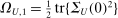 and we use (4.5) and
  . Theorem 2 (i) follows, if we prove
 (B.22)
 (B.23)
 can be rewritten as

 converges in probability to 1 from (B.23), the term within the curly brackets in the first line in the r.h.s. converges in distribution to a standard normal distribution from (B.21), and the term on the second line on the r.h.s. is
  from (B.22).
Le us now prove equations (B.22) and (B.23) by deriving the asymptotic expansions of  and
and  . To derive the asymptotic expansion of
  , we use its definition
  , where the matrices
  ,
,  , involve the estimated loadings and residuals. We plug in the uniform asymptotic expansions from Proposition D.4(ii) in OA Section D.4 to show the next result.
Lemma B.8.Under Assumptions A.1–A.9: (i) The asymptotic expansion of estimator  is
is
 (B.24)
 , where
  with
with  , and
, and  and
and
 (B.25)
 ,
,  are nonsingular matrices w.p.a. 1. (ii) The asymptotic expansion of
  is
is
 (B.26)
 , where
  , with
  , and
, and  .
.
 by matrix inversion:
 (B.27)
 and rearranging terms, we get

 and
and  in Lemma B.8, we have
 (B.28)
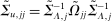 and
and  , for
, for  . In particular, the upper-left
  block of
  vanishes, that is,
  for
for  .
.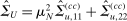 :
:
 (B.29)
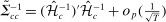 . This equation, together with the asymptotic expansion (B.29) and the commutative property of the trace operator, imply equation (B.22). Similarly, the asymptotic expansion (B.29) and the convergence
  imply equation (B.23).
B.2.2 Proof of Part (ii)
In order to prove Theorem 2 (ii), we consider the behavior of statistic  under the alternative hypothesis
  of less than
  common factors. Specifically, let
  be the true number of common factors in the DGP. The statistic is given by
  . We rely on the following lemma. For its proof, we assume that
  is used to estimate the common factor in panel
  , while estimator
  is used in panel
  .
.
Lemma B.9.Under the alternative hypothesis  , with
  , we have
  , w.p.a. 1, for a constant
  .
.
 , where the
  term follows from the continuity of the eigenvalues mapping, we get
  . Under
  , we have
  canonical correlations that are equal to 1, while the other ones are strictly smaller than 1. Therefore,
  . Then, from Lemma B.9, we get
  , w.p.a. 1, for a constant
  . The conclusion follows.