Preferences for Truth-Telling

1.1 Design

The meta study covers 90 experimental studies containing 429 treatment conditions that fit our inclusion criteria. We include all studies using the setup introduced by Fischbacher and Föllmi-Heusi (2013) (which we will refer to as “FFH paradigm”). Subjects conduct a random draw and then report their outcome of the draw, that is, their state. We require that the true state is unknown to the experimenter (i.e., we require at least two states) but that the experimenter knows the distribution of the random draw. We also include studies in which subjects report whether their prediction of a random draw was correct (as in Jiang (2013)). The payoff from reporting has to be independent of the actions of other subjects, but the reporting action can have an effect on other subjects. The expected payoff level must not be constant, for example, no hypothetical studies, and subjects are not allowed to self-select into the reporting experiment after learning about the rules of the experiment. We only consider distributions that either (i) have more than two states and are uniform or symmetric single-peaked, or (ii) have two states (with any distribution). This excludes only a handful of treatments in the literature. For more details on the selection process, see Appendix A.

We contacted the authors of the identified papers and obtained the raw data of 54 studies. For the remaining studies, we extract the data from graphs and tables shown in the papers. This process does not allow to recover additional covariates for individual subjects, like age or gender, and we cannot trace repeated decisions by the same subject. However, for most of our analyses, we can reconstruct the relevant raw data entirely in this way. The resulting data set thus contains data for each individual subject. Overall, we collect data on 270,616 decisions by 44,390 subjects. Experiments were run in 47 countries which cover 69 percent of world population and 82 percent of world GDP. A good half of the overall sample are students; the rest consists of representative samples or specific non-student samples like children, bankers, or nuns. Table I lists all included studies. Studies for which we obtained the full raw data are marked by *.

Having access to the (potentially reconstructed) raw data is a major advantage over more standard meta studies. We can treat each subject as an independent observation, clustering over repeated decisions and analyzing the effect of individual-specific covariates. We can separately use within-treatment variation (by controlling for treatment fixed effects), within-study variation (by controlling for study fixed effects), and across-study variation for identification. Most importantly, we can conduct analyses that the original authors did not conduct. For other meta studies using the full individual subject data (albeit on different topics), see, for example, Harless and Camerer (1994), Weizsäcker (2010), or Engel (2011).

Since the potential reports differ widely between studies, for example, sides of a coin or color of balls drawn from an urn, we focus on the payoff consequences of a report as its defining characteristic. To make the different studies comparable, we map all reports into a “standardized report.” Our standardized report has three key properties: (i) if a subject's report leads to the lowest possible payoff, the standardized report is −1, (ii) if the report leads to the highest possible payoff, it is +1, and (iii) if the report leads to the same payoff as the expected payoff from truthful reporting, the standardized report is 0. In particular, we define

where π is the payoff of a given report, is the payoff from reporting the lowest possible state, is the payoff from reporting the highest state, and is the expected payoff from truthful reporting. For example, a roll of a six-sided die would result in standardized reports of −1, −0.6, −0.2, +0.2, +0.6, or +1.

In general, without making further assumptions, one cannot say how many people lied or by how much in the FFH paradigm. We can only say how much money people left on the table. An average standardized report greater than 0 means that subjects leave less money on the table than a group of subjects who report fully honestly.

To give readers the possibility to explore the data in more detail, we have made interactive versions of all meta-study graphs available at www.preferencesfortruthtelling.com. The graphs allow restricting the data, for example, only to specific countries. The graphs also provide more information about the underlying studies and give direct links from the plots to the original papers.

1.2 Results

Figure 1 depicts an overview of the data. Standardized report is on the y-axis and the maximal payoff from misreporting, that is, , is on the x-axis (converted by PPP to 2015 USD). As payoff, we take the expected payoff, that is, the nominal payoff used in the experiment times the probability that a subject receives the payoff, in case not all subjects are paid. Each bubble represents the average standardized report of one treatment. The size of the bubble is proportional to the number of subjects in that treatment. The baseline treatment of Fischbacher and Föllmi-Heusi (2013) is marked in the figure. It replicates quite well.

If all subjects were monetary-payoff maximizers and had no concerns about lying, all bubbles would be at +1. In contrast, we find that the average standardized report is only 0.234. This is significantly () lower than 0.25 or any higher threshold (clustering on subject; 0.38 when clustering on study) and thus bounded away from 1. This means that subjects forego about three-quarters of the potential gains from lying. This is a very strong departure from the standard economic prediction.

This finding turns out to be quite robust. Subjects continue to refrain from lying maximally when stakes are increased. Figure 1 shows that an increase in incentives affects behavior only very little. In our sample, the potential payoff from misreporting ranges from cents to 50 USD (Kajackaite and Gneezy (2017)), a 500-fold increase. In a linear regression of standardized report on the potential payoff from misreporting, we find that a one dollar increase in incentives changes the standardized report by −0.005 (using between-study variation as in Figure 1) or 0.003 (using within-study variation). See Appendix A for more details and for a comparison of our different identification strategies. This means that increasing incentives even further is unlikely to yield the standard economic prediction of +1. In Appendix A, we also show that subjects still refrain from lying maximally when they report repeatedly. In fact, repetition is associated with significantly lower reports. Learning and experience thus do not diminish the effect. Reporting behavior is also quite stable across countries, and adding country fixed effects to our main regression (see Table A.2) increases the adjusted only from 0.370 to 0.457.

We next analyze the distribution of reports within each treatment.

Figure 2 shows the distribution of reports for all experiments using uniform distributions with six or two states, for example, six-sided die rolls or coin flips. We exclude the few studies that have nonlinear payoff increases from report to report. The figure covers 68 percent of all subjects in the meta study (the vast majority of the remaining subjects are in treatments with non-uniform distributions—where Finding 2 also holds). The size of the bubbles is proportional to the number of subjects in a treatment. The dashed line indicates the truthful distribution. The bold line is the average across all treatments, the gray area around it the 95% confidence interval of the average. As one can see in Figure 2, all possible reports are made with positive probability in almost all treatments. More generally, for each distribution of true states we have data on, the likelihood of the modal report is significantly () lower than 0.79 (or any higher threshold), and thus bounded away from 1. We have enough data to cluster on study for the two distributions in Figure 2 and the result is robust to such clustering.

The figure also shows that reports that lead to higher payoffs are generally made more often, both for six-state and two-state distributions. The right panel of Figure 2 plots the likelihood of reporting the low-payoff state (standardized report of −1) for two-state experiments. The vast majority of the bubbles are below 0.5, which implies that the high-payoff report is above 0.5. This positive correlation between the payoff of a given state and its likelihood of being reported holds for all uniform distributions we have data on (OLS regressions, all ). We have enough data for the distributions with two, three, six, and 10 states to test report-to-report changes, and find that the reporting likelihood is strictly increasing for two, three, and six states (all ) and weakly increasing for 10 states. We have enough data to cluster on study for two- and six-state distributions and the result is robust to such clustering.

Interestingly, some reports that do not yield the maximal payoff are reported more often than their truthful probability; in particular, the second highest report in six-state experiments is more likely than 1/6 in almost all treatments. Such over-reporting of non-maximal states occurs in all distributions with more than three states we have data on (see Figure A.7 for the uniform distributions). We test all non-maximal states that are over-reported against their truthful likelihood using a binomial test. The lowest p-value is smaller than 0.001 for all distributions (we exclude distributions for which we have very little data, in particular, only one treatment). We have enough data to cluster on study for the uniform six state distribution and the result is robust to such clustering.

We relegate additional results and all regression analyses to Appendix A.

2.1 Theoretical Framework

An individual observes state , drawn i.i.d. across individuals from distribution F (with probability mass function f). We will suppose, except where noted, that the drawn state is observed privately by the individual. We suppose is a subset of equally spaced natural numbers from to , ordered with . As in the meta study, we only consider distributions F that have for all and that either (i) have more than two states and are uniform or symmetric single-peaked, or (ii) have two states (with any distribution). Call this set of distributions .6 After observing a state, individuals publicly give a report , where is a subset of equally spaced natural numbers from to , ordered . Individuals receive a monetary payment which is equal to their report r. We suppose that there is a natural mapping between each element of and the corresponding element of .7 For example, imagine an individual privately flipping a coin. If they report heads, they receive £10; if they report tails, they receive nothing. Then , and . We denote the distribution over reports as G (with probability mass function g). An individual is a liar if they report . The proportion of liars at r is .

We denote a utility function as ϕ. For clarity of exposition, we suppose that ϕ is differentiable in all its arguments, except where specifically noted, although our predictions are true even when we drop differentiability and replace our current assumptions with the appropriate analogues (we do maintain continuity of ϕ). We will also suppose, except where specifically noted, that sub-functionals of ϕ are continuous in their arguments.

We suppose that individuals are heterogeneous. They have a type , where is a vector with J entries, and Θ is the set of potential types , with . Each of the J elements of gives the relative trade-off experienced by an individual between monetary benefits and specific non-monetary, psychological costs (e.g., the cost of lying, or reputational costs). When we introduce specific models, we will only focus on the subvector of that is relevant for each model (which will usually contain only one or two entries). We suppose that is drawn i.i.d. from H, a non-atomic distribution on Θ. Each entry is thus distributed on .8 In Appendix E, we show that the set of non-falsified models does not change if we assume that H is degenerate. The exogenous elements of the models are thus the distribution F over states and the distribution H over types, while the distribution G over reports and thus the share of liars at r, , arise endogenously in equilibrium.

We assume that individuals only report once and there are no repeated interactions. We suppose a continuum of “subject” players and a single “audience” player (the continuum of subjects ensures that any given subject has a negligible impact on the aggregate reporting distribution). The subjects are individuals exactly as described above. The audience takes no action, but rather serves as a player who may hold beliefs about any of the subjects after observing the subjects' reports. The audience could, for example, be the experimenter or another person the subject reveals their report to. Subjects do not observe each others' reports. Utility may depend on the distribution of others' reports, the drawn state-report combinations of others, or beliefs.9 Because subjects take a single action, we can consider a strategy as mapping type and state combinations () into a distribution over reports r.10 When an individual's utility depends on the beliefs of other players, we consider the Sequential Equilibria of the induced psychological game, as introduced by Battigalli and Dufwenberg (2009). (The original psychological game theory framework of Geanakoplos, Pearce, and Stacchetti (1989) cannot allow for utility to depend on updated beliefs.) When utility does not depend on others' beliefs, the analysis can be simplified and we assume the solution concept to be the set of standard Bayes Nash Equilibria of the game. In some of our models, an individual's utility depends only on their own state and report. In this case, our solution concept is simply individual optimization, but for consistency, we also use the words equilibrium and strategy to describe the outcomes of these models.

2.2 Modeling Preferences for Truth-Telling

In this section, we introduce one example for each of the three main categories of lying aversion: lying costs (Section 2.2.1), social norms/comparisons (2.2.2), and reputational concerns (2.2.3). The remaining models are described in Appendix B. Some of these models represent other ways of formalizing the effect of descriptive norms and social comparisons on reporting, including a model of inequality aversion (Appendix B.1); a model that combines lying costs with inequality aversion (B.2); and a social comparisons model in which only subjects who could have lied upwards matter for social comparisons (B.3). Other models build on the idea of reputational concerns and include a model where individuals want to signal to the audience that they place low value on money (B.4); a model where individuals want to cultivate a reputation as a person who has high lying costs (B.5); and a model of guilt aversion (B.6). Finally, we include a model of money maximizing with errors (B.7), and a model that combines lying costs with expectations-based reference-dependence (B.8). In addition, Appendix C describes several models that fail to explain the findings of the meta study and that are therefore not further considered in the body of the paper. Most prominently, we discuss a model in which individuals only care about the audience's belief about their honesty (Appendix C.2).

2.2.1 Lying Costs (LC)

A common explanation for the reluctance to lie is that deviating from telling the truth is intrinsically costly to individuals. The fact that individuals' utility also depends on the realized state, not just their monetary payoff, could come from moral or religious reasons; from self-image concerns (if the individual remembers ω and r);11 from “injunctive” social norms of honesty, that is, norms that are based on a shared perception that lying is socially disapproved; or from the unwillingness to defy the authority of the person or institution who asks for the private information. Such “lying-cost” (LC) models have wide popularity in applications and represent a simple extension of the standard model in which individuals only care about their monetary payoff. Our formulation of this class of models nests all of the lying cost models discussed in the literature, including a fixed cost of lying, a lying cost that is a convex function of the difference between the state and the report, and generalizations that include different lying-cost functions.12

Formally, we suppose individuals have a utility function

c is a function that maps to the (weak) positive reals and denotes the cost of lying. We suppose that c has a minimum when , which is not necessarily unique. (For some specifications, for example fixed costs of lying, c will not be differentiable in its arguments.) For our calibrational exercises, we normalize , so that individuals experience no cost when they tell the truth. In order to make the model non-trivial, we suppose that there is at least one non-maximal state ω such that there exists an where 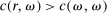(otherwise, no one would ever pay any costs to lying). The only element of that affects utility is the scalar which governs the weight that an individual applies to the lying cost. We make a few assumptions on ϕ. First, ϕ is strictly increasing in the first argument, fixing all the other arguments; this captures the property that utility is increasing in the monetary payment received. Second, ϕ is decreasing in the second argument, fixing all the other arguments, capturing the property that utility falls as the cost of lying increases. In particular, it is strictly decreasing for all . Third and fourth, fixing all other arguments, ϕ is (weakly) decreasing in , and the cross partial of ϕ with respect to c and is strictly negative, while other cross partials are 0. This captures the properties that an individual with a higher draw of has both a higher utility cost of lying, for the same “sized” lie, and faces a higher marginal cost of lying. In other words, utility exhibits increasing differences with respect to c and .13 The solution to LC models can be found by simply solving a single decision maker's optimization problem.

2.2.2 Social Norms: Conformity in LC

Another potential explanation for lying aversion extends the intuition of the LC model. It posits that individuals care about social norms or social comparisons which inform their reporting decision. The leading example is that individuals may feel less bad about lying if they believe that others are lying, too. Importantly, the norms here are “descriptive” in the sense that they are based on the perception of what others normally do, rather than “injunctive,” which are instead based on the perception of what ought to be done and do not depend on the behavior of others (injunctive norms are better captured by LC models). We call such a model “Conformity in LC.” Such concerns for social norms are discussed, for example, in Gibson, Tanner, and Wagner (2013), Rauhut (2013), and Diekmann, Przepiorka, and Rauhut (2015). Our model follows the intuition of Weibull and Villa (2005). We suppose that an individual's total utility loss from misreporting depends both on an LC cost (as described in the previous model), but also on the average LC cost in society. The latter depends not just on players' actions, but on the profile of joint state-report combinations across all individuals. Because we can think of any individual's drawn state as part of their privately observed type, we use the framework of Bayes Nash Equilibrium.14

Formally, in the Conformity in LC model, individuals have a utility function

has the same interpretation and assumptions as in the LC model and types are heterogeneous in the scalar (where CLC denotes the “Conformity in LC” model specific parameter; analogous abbreviations are used for the rest of the models); the rest of the vector again does not affect utility. is the average incurred LC cost in society. This average cost is determined in equilibrium, and thus all individuals know what it is; for notational ease, we suppress the dependence of on the other parameters of the model. η captures the “normalized cost of lying,” that is, the cost of lying conditional on the incurred LC cost in society (for our calibrational exercises, we suppose ) and is strictly increasing in its first argument. For , η is strictly falling in the second argument so that the normalized cost is increasing in the individual's own personal lying cost and falling in the aggregate LC cost, that is, their lying costs are falling as others lie more (for , the partial of η with respect to its second argument is 0). As in the previous model, ϕ is strictly increasing in its first argument, and decreasing in the second argument (strictly so for all ). ϕ is (weakly) decreasing in fixing the first two arguments, and the cross partial of ϕ with respect to η and is strictly negative, while other cross partials are 0. These assumptions are analogous to the ones presented in the previous models and capture the same intuitions.

2.2.3 Reputation for Honesty + LC

A different way to extend the LC model is to allow individuals to experience both an intrinsic cost of lying, as well as reputational costs associated with inference about their honesty (e.g., Khalmetski and Sliwka (forthcoming), Gneezy, Kajackaite, and Sobel (2018)). We suppose that an individual's utility is falling in the belief of the audience player that the individual's report is not honest, that is, has a state not equal to the report. Akerlof (1983) provided the first discussion in the economics literature that honesty may be generated by reputational concerns, and many recent papers have built on this intuition.15 Thus, an individual's utility is belief-dependent, specifically depending on the audience player's updated beliefs. Thus, we must use the tools of psychological game theory to analyze the game. We use the framework of Battigalli and Dufwenberg (2009) in our analysis.16 Of course, the audience cannot directly observe whether a player is lying, and has to base their beliefs on the observable report r. Utility is thus a decreasing function of the audience's belief about whether an individual lied. Because the audience player makes correct Bayesian inference based on observing the report and knowing the equilibrium strategies, their posterior belief about whether an individual is a liar, conditional on a report r, is , the fraction of liars at r in equilibrium. We therefore directly assume that utility depends on , with υ a strictly increasing function.

Since lying costs are our preferred way to capture self-image concerns about honesty, one possible interpretation of this model is that individuals care about self-image and social image (i.e., the audience's beliefs). We focus on a situation where there is additive separability between the different components of the utility function.17 Formally, in the “Reputation for Honesty + LC” model, utility is

u is strictly increasing in r. Types are heterogeneous in the scalars and and the rest of does not affect utility. c is as described in the LC model. υ is a strictly increasing function of with a minimum at 0 (and in calibrational exercises, we normalize . Thus, the individual likes more money, but dislikes lying and being perceived as a liar by the audience. The functional form implies analog patterns for the cross partials as the previous models.18

2.3 Distinguishing Models Using the Meta Study

We now turn to understanding how our models can be distinguished in the data. The first test is whether the models can match the four findings of the meta study. We find that the three models presented in the previous section, as well as all those listed in Appendix B, can do so.

All proofs for the results in this section are collected in Appendix D. The proof for the LC model constructs one example utility function, combining a fixed cost and a convex cost of lying, and then shows that it yields Findings 1–4 for any n and any . Many of the other models considered in this paper contain the LC model as limit case and can therefore explain Findings 1–4. However, there are several models, for example, the Inequality Aversion model (Appendix B.1) or the Reputation for Being Not Greedy model (B.4), which rely on very different mechanisms and can still explain Findings 1–4.

2.4 Distinguishing Models Using New Empirical Tests

Proposition 1 shows that the existing literature, reflected in the meta study, cannot pin down the mechanism which generates lying aversion. The meta study does falsify quite a few popular models, which we discuss in Appendix C, but the data are not strong enough to narrow the set of surviving models further down. This motivates us to devise four additional empirical tests which can distinguish between the models that are in line with the meta study. Three of the four new tests are “comparative statics” and one is an equilibrium property: (i) how does the distribution of true states affect the distribution of reports; (ii) how does the belief about the reports of other subjects influence the distribution of reports; (iii) does the observability of the true state affect the distribution of reports; (iv) will some subjects lie downwards if the true state is observable. As a prediction (iv′), we also derive whether some subjects will lie downwards if the true state is not observable, as in the standard FFH paradigm. We cannot test this last prediction in our data but state it nonetheless as it is helpful in building intuition regarding the models as well as important for potential applications.19

We derive predictions for each model and for each test using very general specifications of individual heterogeneity and the functional form. We present predictions for an arbitrary number of states n and for the special case of . On the one hand, allowing for an arbitrary number of states generates predictions that are applicable to a larger set of potential settings. On the other hand, restricting allows us to make sharper predictions, and thus potentially falsify a larger set of models. For example, for models where individuals care about what others do (e.g., social comparison models), it does not matter whether individuals care about the average report or the distribution of reports when . For models that rule out downwards lying, the binary setting also allows us to back out the full reporting strategy of individuals without actually observing the true state: the high-payoff state will be reported truthfully, so we can deduct the expected number of high-payoff states from the number of observed high-payoff reports and we are left with the reports made by the subjects who have drawn the low-payoff state. Moreover, conducting our new tests with two-state distributions is simpler and easier to understand for subjects. Recall that across all results, we only consider distributions .

The models, as well as the predictions they generate in each of the tests, are listed in Table II. We report the two-state predictions in the columns describing the effect of shifts in the distributions of true states F and beliefs about others' reports (see below for details), since we use two-state distributions in our new experimental tests of these predictions. Some of the models we consider do not guarantee a unique reporting distribution G without additional parametric restrictions. We discuss below in more detail how we deal with potential non-uniqueness for each prediction and we mark the models which do not necessarily have unique equilibria with an asterisk (*) in Table II. Importantly, no model is ruled out solely on the basis of predictions that are based on an assumption of uniqueness. Similarly, the models that cannot be falsified by our data are not consistent solely because of potential multiplicity of equilibria.

We now turn to discussing our four empirical tests. The first test is about how the distribution of reports G (recall that gives the unconditional fraction of individuals giving report ) changes when the higher states are more likely to be drawn (but while maintaining the same set of support for the distribution). Specifically, we suppose that we induce a shift in the distribution of states F (recall that gives the probability that state is drawn) that satisfies first-order stochastic dominance. We then look at 1 minus the ratio of the observed number of reports of the lowest state to the expected number of draws of the lowest state: 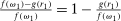. For those models in which no individual lies downwards, we can interpret the statistic as the proportion of people who draw but report something higher, that is .

Thus, the term “drawing in” means that the lowest state is even more under-reported when higher states become more likely. “Drawing out” refers to the opposite tendency. As we will show below, several very different motivations can lead to drawing in. For example, increasing the true probability of high states increases the likelihood that a high report is true, leading subjects who care about being perceived as honest, as in our Reputation for Honesty + LC model (Section 2.2.3), to make such reports more often. But increasing the true probability of high states also increases the likelihood that other subjects report high, pushing subjects who dislike inequality (Appendix B.2) to report high states. And subjects who compare their outcome to their recent expectations (Appendix B.8) could also react in this way.20

The second test looks at how an individual's probability of reporting the highest state will change when we exogenously shift their belief about the distribution of reports. We will refer to as the beliefs of players about the distribution of reports. In equilibrium, given correct beliefs about others, . Our experiment focuses on manipulating the beliefs about others, that is, , so that they may no longer be correct, and then observing the resulting actual reporting distribution G. We focus on situations where there is full support on all reports in both beliefs and actuality.

Thus, the term “affinity” means that reporting of the highest state increases when the subject believes that higher states are more likely to be reported by others. The term “aversion” refers to the opposite tendency. Such an exercise allows us to test the models in one of three ways. First, in some models, for example, Inequality Aversion (Appendix B.1), individuals care directly about the reports made by others and thus (or a sufficient statistic for it) directly enters the utility. Therefore, we can immediately assess the effect of a shift in on behavior.21 For these models, shifting an individual's belief about directly alters their best response (and since subjects are best responding to their , which may be different from the actual G, we may observe out-of-equilibrium behavior). These models all predict affinity.

Second, in some other models (Conformity in LC and Censored Conformity in LC), individuals care about the profile of joint state-report combinations across other individuals (i.e., the amount of lying by others). In these models, no individual lies downwards and so, for binary states, contains sufficient information about the joint state-report combinations. Thus, shifting directly alters an individual's best response. These models again predict affinity.

Finally, this exercise allows us, albeit indirectly, to understand what happens when beliefs about H (the distribution of ) change. Directly changing this belief is difficult since this requires identifying for each subject and then conveying this insight to all subjects. However, for models with a unique equilibrium, because G is an endogenous equilibrium outcome, shifts in can only be rationalized by subjects as shifts in some underlying exogenous parameter—which has to be H, since our experiment fixes all other parameters (e.g., F and whether states are observable).22 For many of these models, the conditions defining the unique equilibrium reporting strategy are invariant to shifts in and H, which means that our treatment should not affect behavior. For another set of models, in particular Reputation for Being Not Greedy, Reputation for Honesty + LC, and LC-Reputation, there is no simple mapping from to beliefs about H and a shift in could lead to affinity, aversion, or -invariance.

Our third test considers whether or not it matters for the distribution of reports that the audience player can observe the true state. In particular, we will test whether individuals' reports change if the experimenter can observe not only the report, but also the state for each individual.

In some of the models we consider, the costs associated with lying are internal and therefore do not depend on whether an audience is able to observe the state or not. In other models, however, the costs depend on the inference the audience is able to make, and so observability of the true state affects predictions.23

Our fourth test comes in two parts. Both parts try to understand whether or not there are individuals who engage in downwards lying, that is, draw and report with . The first is whether downwards lying can occur in an equilibrium with observability of the state by the audience and where G features full support. The second is an analogous test but in the situation where the state is not observed by the audience. We will only focus on the former test in our experiments.

Although lying down may seem counterintuitive, as we will show below, there can be a number of reasons why individuals may want to lie downwards. In models where individuals are concerned with reputation, lying downwards may be beneficial if low reports are associated with a better reputation than high reports. Alternatively, in models of social comparisons, such as the inequality aversion models, downwards lying may arise because individuals aim to conform to others' reports.

The following proposition summarizes the predictions for the three models described above.

“Depending on parameters” refers to the distribution over states F, the distribution H over types, any sub-functions that might be introduced in a model definition, for example, the cost function c in the LC model, and when considering affinity, aversion, and -invariance, (as this is something we experimentally manipulate). In the cases when predictions depend on parameters, the proofs will provide examples for each possible behavior. If the statement is unqualified, it means that it holds for any , any H, sub-functions, and .

Before moving on, we provide some intuition for the results. For simplicity, we focus on two-state/report distributions. In the LC model, individuals never lie downwards, because they (weakly) pay a lying cost and also receive a lower monetary payoff when doing so. Since only their own state and their own report matter for utility, conditional on drawing the low state, for a fixed , an individual will always make the same report, regardless of F or . Thus, we observe both f-invariance and -invariance. Last, the lying cost is an internal cost and does not depend on the inference others are making about any given person. Thus, individuals do not care whether their state is observed.

In the Conformity in LC models, individuals will never lie downwards since, as in the LC model, they would face a lower monetary payoff as well as a weakly higher cost of lying. Morever, with a unique equilibrium, as increases, more individuals draw the high state and can report without having to lie. Thus, the average incurred cost of lying falls. This increases the normalized cost of lying (η) for all individuals. Thus, an individual who draws , and was indifferent before between and , will now strictly prefer . This implies drawing out. In the Conformity in LC model, because G enters directly into the utility function and because no one lies downwards, we can tell how the individual's best response changes with shifts in expected G, that is, . Fixing F, if increases, more people draw the low state but say the high report. This means that more individuals are expected to lie, and so the normalized cost of lying (η) decreases. Thus, individuals who draw the low report will be more likely to say the high report, that is, we have affinity. Last, as in the LC model, these costs do not depend on any inference others are making, and so individuals do not care whether their state is observed.

In the Reputation for Honesty + LC model, because individuals have a concern for reputation and also have lying costs, they may or may not lie down if the state is unobserved. If an individual is motivated relatively more by reputational concerns, then they will lie down if the state is unobserved. In contrast, if lying costs dominate as a motivation, they will not lie down. If the state is observed, no one lies downwards. Although multiple equilibria may occur, whenever the equilibrium is unique, the Reputation for Honesty + LC model exhibits drawing in. As increases, some individuals who previously drew will now draw . Those individuals now face a lower LC cost when giving the high report (which is in fact zero). Fixing the reputational cost, this implies some of them will now give the high report (instead of the low report). Fixing the behavior of others, this reduces the fraction of liars giving the high report and thus the reputational cost of the high report decreases; and similarly, increases the fraction of liars giving the low report. This reduces the (relative) cost of giving the high report even more. Therefore, we observe drawing in. Our intuition here relies on partial equilibrium reasoning, but the formal proof shows how to extend this to full equilibrium reasoning. Even with a unique equilibrium, we may observe either aversion, affinity, or -invariance since it depends on how the distribution of H is perceived to have changed when shifts.24 Because the model includes reputational costs, whether or not the audience observes just the report, or also the state, matters for behavior.

In Appendix F, we provide additional evidence regarding predictions of the Kőszegi–Rabin + LC model which are not listed in the table. We also test specific f-invariance predictions for the LC model in a 10-state experiment, where we show that drawing-in like behavior also obtains in an experiment with 10 states.

3.1 Shifting the Distribution of True States F

We test the effect of a shift in the distribution of true states F using treatments with two-state distributions. Subjects are invited to the laboratory for a short session in which they are asked to complete a questionnaire that contains some basic socio-demographic questions as well as filler questions about their financial status and money-management ability that serve to increase the length of the questionnaire so that the task appears meaningful. Subjects are told that, they would receive money for completing the questionnaire and that the exact amount would be determined by randomly drawing a chip from an envelope. The chips have either the number 4 or 10 written on them, representing the amount of money in GBP that subjects are paid if they draw a chip with that number. Thus, drawing a chip with 4 on it represents drawing and drawing a chip with 10 represents drawing . Reports of 4 and 10 are similarly and . The chips are arranged on a tray on the subject's desk such that subjects are fully aware of the distribution F (see Appendix G for a picture of the lab setup). Subjects are told that, at the end of the questionnaire, they need to place all chips into a provided envelope, shake the envelope a few times, and then randomly draw a chip from the envelope. They are told to place the drawn chip back into the envelope and to write down the number of their chip on a payment sheet. Subjects are then paid according to the number reported on their payment sheet by the experimenter who has been waiting outside the lab for the whole time.

We conduct two between-subject treatments, varying the distribution of chips that subjects have on their trays. In one treatment, the tray contains 45 chips with the number 4 and 5 chips with the number 10. In the other treatment, the tray contains 20 chips with the number 4 and 30 chips with the number 10. We label the two treatments F_LOW and F_HIGH, respectively, to indicate the different probabilities of drawing the high state (10 percent vs. 60 percent). Note that the distribution used in F_HIGH first-order stochastically dominates the distribution in F_LOW in line with Definition 1. We select samples sizes such that the expected number of low states is the same (and equal to 131) in the two treatments. Thus, we have 146 subjects in F_LOW and 328 subjects in F_HIGH. Most of the sessions were conducted in Nottingham and some in Oxford between June and December 2015.

3.2 Results

Figure 3 shows the values of the statistic across the two treatments. In F_LOW, we expect 131 subjects to draw the low £4 payment and we observe 80 subjects actually reporting 4, that is, our statistic is equal to . In F_HIGH, we also expect 131 subjects to draw 4, but only 43 subjects report to have done so, so our statistic is equal to 0.67 (this means that 45 percent of subjects in F_LOW and 87 percent in F_HIGH report 10). This difference of almost 30 percentage points is very large and highly significant (, OLS with robust SE; , test).25

3.3 Shifting Beliefs About the Distribution of Reports

Our next set of treatments is designed to test predictions concerning the effects of a shift in subjects' beliefs about the distribution of reports, that is, . There are three other studies testing the effect of beliefs on reporting (Rauhut (2013), Diekmann, Przepiorka, and Rauhut (2015), and Gächter and Schulz (2016a)). These studies affect beliefs by showing to subjects the actual past behavior of participants. Diekmann, Przepiorka, and Rauhut (2015) and Gächter and Schulz (2016a) found no effect and Rauhut (2013) found a positive effect. Rauhut (2013), however, compared subjects who have initially too high beliefs that are then updated downwards to subjects who have initially too low beliefs that are updated upwards. The treatment is thus not assigned fully randomly.

We use an alternative and complementary method. Our strategy to shift beliefs is based on an anchoring procedure (Tversky and Kahneman (1974)): we ask subjects to think about the behavior of hypothetical participants in the F_LOW experiment and we anchor them to think about participants who reported the high state more or less often. The advantage of our design is that we do not need to sample selectively from the distribution of actual past behavior of other subjects. This could be problematic because, if the past behavior is highly selected but presented as if representative, it could be judged as implicitly deceiving subjects and could confound results of an experimental study on deception. We are not aware of other studies that have used anchoring to affect beliefs before.

In our setup, subjects are asked to read a brief description of a “potential” experiment which follows the instructions used in the F_LOW experiment, that is, 90 percent probability of the low payment and 10 percent probability of the high payment. Subjects also have on their desk the tray with chips and envelope that subjects in the F_LOW experiment had used. Subjects are then asked to “imagine” two “possible outcomes” of the potential experiment. There are two between-subject treatments, varying the outcomes subjects are asked to imagine. In treatment G_LOW, the outcomes have 20 percent and 30 percent of hypothetical participants reporting to have drawn a 10, while in treatment G_HIGH, these shares are 70 percent and 80 percent. Subjects are then asked a few questions about these outcomes.26 Subjects are then told that the experiment has actually been run in the same laboratory in the previous year and they are asked to estimate the fraction of participants in the actual experiment who have reported a 10. Subjects are paid £3 if their estimate is correct (within an error margin of ±3 percentage points). This mechanism is very simple and easier to explain and understand than proper scoring rules. It elicits in an incentive-compatible way the mode (or more precisely, the mid-point of the 6-percentage point interval with the highest likelihood) of a subject's distribution of estimates. We use subjects' estimates to check whether our anchoring manipulation is successful in shifting subjects' beliefs.27

Finally, after answering a few additional socio-demographic questions, subjects are told that they will be paid an additional amount of money on top of their earnings from the belief elicitation. To determine how much money they are paid, subjects are asked to take part in the F_LOW experiment themselves. The procedure is identical to the description of F_LOW in the previous section. The experiments were conducted in Nottingham between March and May 2016 with a total of 340 subjects (173 in G_LOW, 167 in G_HIGH).

3.4 Results

We start by showing the effect of the anchors on subjects' beliefs.

Figure 4 shows the distributions of estimates of the proportion of reported 10's made by subjects across the two treatments. The distribution of the G_HIGH treatment is strongly shifted to the right relative to G_LOW, and practically first-order stochastically dominates it, in line with Definition 2. On average, subjects in G_LOW believe that 41 percent of participants in the F_LOW experiment have reported a 10. In G_HIGH, the average belief is 62 percent (, OLS with robust SE; , Wilcoxon rank-sum test).

Having established that our manipulation is successful in shifting beliefs about reports in the expected direction, our next step is to examine the effects of this shift in beliefs on subjects' actual reporting behavior.

Figure 5 shows the share of subjects reporting a 10 across the two treatments. Recall that, in both treatments, the true probability of drawing a 10 is 10 percent (this is indicated by the dashed line in the figure). We observe 55 percent of subjects reporting a 10 in G_LOW, and 49 percent in G_HIGH. This difference is not significant (, OLS with robust SE; , 2SLS regressing report on belief with treatment as instrument for belief; , test). Taken together, our study and the previous literature provide converging evidence that manipulating beliefs about others' reports has a limited impact on reporting.

One word of caution is warranted. Even though the point estimate of the effect of the treatments is quite close to zero, we cannot reject (small) positive or negative effects of a change in beliefs. A power analysis shows that we can only detect treatment differences of 15 percentage points or larger at the 5% level and with 80% power, but we are not sufficiently powered to detect small differences like that observed in Figure 5. This may raise the concern that our rejection of many models, in particular the social comparisons models, which all predict affinity, is driven by a lack of power. However, these models typically predict quite large responses to shifts in . For example, a simple, calibrated version of the Conformity in LC model implies that 21 percent of subjects should increase their reports across our treatments, which we do have power to detect. In fact, our data show that (in net) 6 percent of subjects decrease their report.28

3.5 Changing the Observability of States

A final set of treatments tests whether observability of the subject's true state by the experimenter affects reporting behavior, in line with Definition 3. The experiments use a setup similar to the one described above. Subjects are invited to the lab to fill in a questionnaire and are paid based on a random draw that they perform privately. There are two between-subject treatments. Differently from the previous experiments, in both treatments the draw is performed out of a 10-state uniform distribution. In our UNOBSERVABLE treatment, the draw is performed using the same procedures described for the previous experiments: subjects draw a chip at random out of an envelope, report the outcome on a payment sheet, and are paid based on this report. Thus, in this treatment, the experimenter cannot observe the true state of a subject and cannot tell for any individual subject whether they lie or tell the truth.

In our OBSERVABLE treatment, we maintain this key feature of the FFH paradigm, but make subjects' true state observable to the experimenter. In order to do so, the procedure of the OBSERVABLE treatment differs from the UNOBSERVABLE treatment in two ways. First, the draw is performed using the computer instead of the physical medium of our other experiments (the chips and the envelope).29 Second, we introduce a payment procedure that makes it impossible for the experimenter to link a report to an individual subject. Before the start of the experiment, the experimenter places an envelope containing 10 coins of £1 each on each subject's desk. Subjects are told to sit “wherever they want” and sit down unsupervised. The experimenter does thus not know which subject is at which desk. After the computerized draw, instead of writing the number on their chip on the payment sheet, subjects are told to take as many coins from the envelope as the number of their chip. Subjects then leave the lab without signing any receipt for the money taken or meeting the experimenter again. At the end of the experiment, the experimenter counts the number of coins left by subjects on each desk to reconstruct their “report” and compares it to the true state drawn on the corresponding computer without being able to link any report to the identity of a subject.30 We ran these experiments at the University of Nottingham with 288 subjects (155 in UNOBSERVABLE; 133 in OBSERVABLE). Experiments were conducted between May and October 2015.

3.6 Results

Figure 6 shows the distribution of reports in the UNOBSERVABLE and OBSERVABLE treatments. The dashed line in the figure indicates that, in both treatments, the truthful probability of drawing each state is 10 percent.

Reports in the UNOBSERVABLE treatment are considerably higher than in the OBSERVABLE treatment ( OLS with robust SE; Kolmogorov–Smirnov test; , Wilcoxon rank-sum test; see Kajackaite and Gneezy (2017) for a similar result).

This result also demonstrates that it would be misleading to rely on evidence from settings in which the true state is observable by the researcher if one is actually interested in understanding a setting in which the true state is truly unobservable.

We can also use the OBSERVABLE treatment to examine our prediction about the existence of downwards lying when the state is observable (Definition 4). Importantly, we may not have the same result in a setting where the true state is unobservable (see Table II).

Figure 7 shows a scatter plot of subjects' reports and true draws in the OBSERVABLE treatment. The size of the bubbles reflects the underlying number of observations. No subject reported a number lower than their true draw, that is, lied downwards. About 60 percent of the subjects who lie report the highest possible number; the remaining 40 percent of liars report non-maximal numbers.

4.1 Overall Result of the Falsification Exercise

Recall that our four empirical tests, in addition to the meta study, concern (i) how the distribution of true states affects one's report (we find drawing in); (ii) how the belief about the reports of other subjects influences one's report (we find -invariance); (iii) whether the observability of the true state affects one's report (we find it does); (iv) whether some subjects will lie downwards if the true state is observable (we find they do not). Taking all evidence together, we find the following:

Table II summarizes the predictions of all models. The two models that cannot be falsified by our data, Reputation for Honesty + LC and LC-Reputation, combine a preference for being honest with a preference for being seen as honest. In Reputation for Honesty + LC, individuals care about lying costs and about the probability of being a liar given their report. In LC-Reputation, individuals care about lying costs and about what an audience observing the report deduces about their lying cost parameter .

All other models fail at least one of the four tests. Looking at Table II, one can discern certain patterns. The LC model, which is most widely used in the literature, fails two tests, predicting f-invariance and o-invariance. The Conformity in LC model, which is our preferred way to model the effect of descriptive norms, fails three tests, predicting drawing out (when the equilibrium is unique), affinity, and o-invariance. All other social comparisons models also predict affinity and o-invariance. Moreover, as we discuss in Appendix C, several popular models, like the standard model and models that assume that subjects only care about their reputation for having been honest, cannot even explain the findings of the meta study (and also fail our new tests).

We find no significant effect of a change in beliefs, that is, -invariance. As we discussed in Section 3.4, our study is sufficiently powered to detect treatment differences implied by reasonably parameterized versions of the social comparison models, for example, Conformity in LC. We cannot, however, rule out (small) positive or negative effects of a change in beliefs. Regardless of whether our treatments have enough power or not, even if we interpreted our data on this test as inconclusive and thus disregard the -invariance result, we can still reject all the social comparisons models because they fail at least one other experimental test.

Importantly, non-uniqueness of equilibria does not affect our overall falsification. Recall that the first and third test might not work when there is more than one equilibrium. All those models that fail the first or third test and could feature multiple equilibria also fail additional tests. Similarly, the models that our data cannot falsify are consistent with the data when the equilibrium is unique.

4.2 A Calibrated Utility Function

In order to demonstrate how one of the non-falsified models, the Reputation for Honesty + LC model (Section 2.2.3), can quantitatively match the data both from the meta study and from our new experiments, we calibrate a simple, linear functional form. Our calibration is not intended to suggest that the functional form presented here, along with our choice of H, best matches the data. Instead, we view this as a demonstration that even quite simple and tractable assumptions generate equilibria that allow us to capture many of the important features of the data. Enriching the model further will only improve the fit. We suggest the following utility function which we call “Calibrated Reputation for Honesty + LC”:

As before, r is the report, ω the true state, and the fraction of liars at r. c is a fixed cost of lying and is an indicator function of whether an individual lied. We suppose all individuals experience the same fixed cost of lying (this utility function is thus a limit case of the Reputation for Honesty + LC model). The individual-specific weight on reputation, , is drawn from a uniform distribution on . The average is thus . Additional details of the calibration are in Appendix H.2.31

We calibrate the model to match the leading example in the literature, a simple die-roll setting, that is, a uniform distribution F over six possible states with payoffs ranging from 1 to 6, where the audience cannot observe the state. We set and . We find that in the equilibrium, no individual lies down. Moreover, for , , and . We find a reporting distribution similar to that found in our meta study: , , , , , and . Figure 8 compares the predicted reporting distribution of this calibrated model to the data. The fit is quite good, in particular given the simple functional form, and the model matches all four findings of the meta study.

It also matches up with our experimental findings. In a setting where the state is observable, the model predicts no downwards lying, as in our data (this is true for all Reputation for Honesty + LC utility functions), and much more truth-telling. Under observability, all liars report the maximal report, similar to our data.

The model also generates the large amount of drawing in we observe. We consider two states like in our F treatments, and in order to keep the payoff scale the same as the previous calibration, we suppose they pay 1 and 6. When , the equilibrium features no lying down and so . Moreover, and the share of low reports is . When , we find two equilibria. One of the equilibria features no lying down, and in this case and . The other equilibrium features lying down; here , , and . Thus, in the last equilibrium, approximately 8 out of every 10 individuals who draw the high state give the low report. For comparison, our experiments yield and , respectively. Regardless of which of these two equilibria is selected, we observe significant amounts of drawing in. Moreover, the model can generate almost any behavior in our treatments, because those treatments do not pin down the belief about H (and thus , on which utility in the model depends). Depending on the new beliefs, aversion, -invariance, or affinity could result, as the new belief could either imply a positive, no, or negative change in the gap between and (see the Reputation for Honesty + LC part of the proof of Proposition 2 for details).

Both components of the utility function are important. In Figure 8, we also plot the predicted reporting distributions for the utility function when we shut down the LC or the RH part. The Only-RH model is far away from the data. The Only-LC model is closer, but this model does not generate drawing in or o-shift.32