Would Hydrologic Climate Changes in Sierra Nevada Streams Influence Trout Persistence?
Abstract
We predicted the consequences of climate change for sympatric populations of brown trout Salmo trutta and rainbow trout Oncorhynchus mykiss in an upstream and a downstream reach of a Sierra Nevada stream with the help of an individual-based trout population model. The model evaluated the ecological effects of two anticipated responses to climate change: (1) a shift in peak flows from spring to winter and (2) an increase in stream temperature. Changes in temperature and flow regime both influenced simulated persistence of the two trout species. We hypothesized a decrease in the fall-spawning brown trout population as a result of winter floods that scour brown trout redds. Although scouring mortality showed the expected pattern, effects of seasonal shifts in flow on simulated dewatering of redds was equally important and tended to compensate for scouring. Because trout are coldwater fishes, we hypothesized that a rise in mean stream temperature would be harmful to both species, particularly in downstream reaches. We found that a climate change scenario with a 2°C increase in average stream temperature benefited both species in the cooler upstream reach but was harmful in the warmer downstream reach. Overall, our results supported the hypothesis that climate change will restrict trout to higher elevations in the Sierra Nevada. Finally, the combined effects of elevated temperature and shifted flow differed from the effect of elevated temperature alone. In combination, the two climatic factors produced threshold effects in rainbow trout abundance by shifting the age at first maturation. Complex interactions between the period of incubation and various causes of redd mortality (dewatering, scouring, and temperature-related mortality) also lead to nonadditive effects of the two climatic factors on abundances. We conclude that focusing on one factor alone (i.e., temperature) may not be sufficient to predict climate change effects in the stream environment.
The effects of climate changes associated with increasing atmospheric CO2 on stream fishes have been studied infrequently. Some studies have predicted that salmonid populations in streams would eventually be fragmented as they are forced to increasingly higher elevations and restricted to headwater streams with maximum summer temperatures below about 21°C (Keleher and Rahel 1996; Rahel et al. 1996). Eaton and Scheller (1996) predicted that coldwater and coolwater species as a whole would lose half of their habitat in U.S. streams. Similarly, Meisner (1990) predicted that southern populations of brook trout Salvelinus fontinalis would lose much of their mid-elevation habitat because of groundwater temperatures above 15°C. All of these studies focused on temperature effects and not on hydrologic effects.
While it is intuitively reasonable to expect that elevated temperatures will be harmful for coldwater species such as trout, it is important to consider other resources and environmental factors that define the realized niche in its natural habitat. For example, Magnuson and DeStasio (1996) predicted that global warming would actually increase the realized niche available to trout in lakes when they considered both dissolved oxygen and temperature. In the stream environment, fish may experience indirect consequences of global warming that are mediated by changes in hydrology and streamflow. There have not been many studies that considered hydrologic effects (e.g., Minns et al. 1995). In this study, we build on predictions of streamflow response to climate change from earlier studies. Lettenmaier and Gan (1990) used the results from general circulation models (GCMs) to predict the effects of doubled atmospheric CO2 on the climate and hydrology of Sierra Nevada streams. They predicted that doubling CO2 will shift the seasonal pattern in streamflow but not the total annual flow. Under current climatic conditions, peak flows generally occur during spring when snow accumulated at higher elevations melts. Under elevated CO2 scenarios, peak flows would occur during rain-on-snow precipitation events in winter. We hypothesized that the fall-spawning brown trout Salmo trutta would be harmed and that the spring-spawning rainbow trout Oncorhynchus mykiss would benefit by this shifted pattern in seasonal flows. We based this expectation on two studies (Seegrist and Gard 1972; Strange et al. 1992) in Sierra Nevada streams. These 10-year studies found that recruitment of fall spawners and spring spawners was correlated with prerecruitment flows.
In this study, we used a trout population model to simulate the consequences of global climate change on coexisting stream populations of brown and rainbow trout. The approach used in this analysis differs from those used in previous studies of climate change effects in four important respects. First, because we used an individual-based population model, we were able to assess the effects of climate on all life stages and to identify the particular mechanisms leading to simulated population change. In addition to growth, we simulated environmental influences on reproduction, incubation, and mortality of older life stages. Shuter and Post (1990) used a similar approach that considered reproductive thresholds, but did not simulate population dynamics. It has been far more common for modeling studies to use a bioenergetics approach focused mainly on temperature effects on growth (e.g., Chang et al. 1992; McDonald et al. 1996; Van Winkle et al. 1997b). Second, by including multiple fish species, the individual-based model has the potential to predict changes in species composition in response to environmental change (e.g., Shugart et al. 1992), recognizing that community interactions also define the realized thermal niche. Third, our model considers streamflow effects in addition to those of elevated stream temperature. Finally, while this study is more local in scale than many climate change studies, we believe that our approach may help to evaluate and stimulate discussion about the relative importance of various processes (e.g., reproduction and early life stages versus adult bioenergetics; autecology versus competitive interactions; flow versus temperature) before extrapolating to a regional scale.
Study Sites
The North Fork Middle Fork (NFMF) of the Tule River is a moderately high-gradient Sierra Nevada stream. Studley et al. (1995: volume 1, section 2) characterized four reaches ranging from above the Tule River diversion dam (TRDD) to one below the confluence with Meadow Creek (Figure 1). We selected two reaches for comparison because of the differences in their temperatures. The upstream reach extends 1.9 km between Alder Creek and TRDD and ranges in elevation between 1,292 and 1,220 m. Natural flows above the diversion dam average around 0.85 m3/s and are highest in spring during snowmelt and lowest in summer (Studley et al. 1995; Trihey et al. 1985). The downstream reach runs from the confluence of Meadow Creek to Milk Creek. This segment ranges from 1,117 m to roughly 800 m in elevation. Stream temperatures in the upstream reach typically range from a low of 0°C in winter to a maximum of 18°C in summer, while those below Meadow Creek average 3.1°C higher (Figure 2).
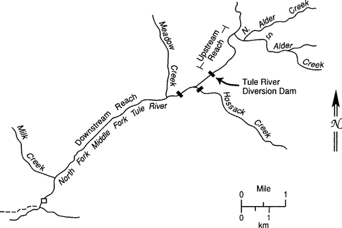
Study sites: an upstream reach and a downstream reach in the Tule River, California
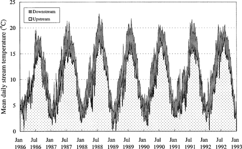
Historical temperatures in an upstream reach and a downstream reach of the Tule River, California. The filled area between the two curves shows the differences between temperatures in the two locations
Habitat Simulation Model
A habitat simulation model generates the spatial setting for trout in our simulations. Its purpose is to produce a realistic “streamscape” of depth and velocity that responds to streamflow. The model translates stream flow into a complex spatial field of velocities and depths that changes daily (see Jager et al. 1993).
To describe the spatial habitat in the Tule River above TRDD, we provided the habitat simulation model with information classifying the stream habitat into a sequence of 119 habitat units belonging to one mesohabitat type (e.g., pool, run, pocket water, riffle, cascade). The habitat simulation model simulated two-dimensional spatial patterns in velocity and depth within each habitat unit as a function of streamflow by using hydraulic relationships estimated from transects at three flows ranging from 0.17 to 1.1 m3/s. For example, in the upstream reach we used hydraulic data from 12 transects representing all of the mesohabitat types and containing 30–50 stations each. Other characteristics of the habitat units provided in the habitat map used by the model, for a single reference flow, were unit length, mean width, mean depth, percent instream cover, percent spawning habitat, and slope.
Because hydraulic survey data were not available for every habitat unit in the stream, we used hydraulic data from a habitat unit that has hydraulic data and that is of the same mesohabitat type and similar dimensions. The model partitions each habitat unit into a two-dimensional grid of model cells centered on the measurement stations. Cells were typically less than 1 m wide and extended the full length of the habitat unit. The habitat simulation model simulated the depth and average water column velocity for each cell as a function of flow in each pool, run, pocket water, and riffle, but not in cascades and other habitat units too steep to model hydraulically or to provide fish habitat.
In most respects, the approach is identical to the hydraulic simulation component of the physical habitat simulation (PHABSIM) model's IFG4 program developed by Milhous et al. (1989). We used PHABSIM software to estimate hydraulic parameters that relate depth and velocity to flow (see equations and description in the Appendix).
Trout Population Model
Model description
The population model that we used to simulate brown and rainbow trout is individual-based and spatially explicit. A complete description of the model and its calibration in the Tule River, California, has been published elsewhere (Van Winkle et al. 1996, 1998).
Spawning
Brown trout are fall spawners, and native rainbow trout spawn in spring. Temperature controls the timing of spawning within a seasonal window determined by photoperiod (day length). We restrict brown trout spawning to a narrower range of day lengths than we do the more flexible rainbow trout. Within this spawning window, the exact spawning date for each mature individual is determined by its assigned temperature threshold. In addition, spawning may be delayed by high flows. For these climate change simulations, we were careful to allow rainbow trout to reproduce earlier in response to elevated temperatures as this was the response observed by Kaya (1977) in a geothermal spring. For individual model trout that are in good condition, the likelihood of spawning increases linearly as a function of length. This likelihood increases from 0 to 1 between 180 mm and 210 mm for brown trout and between 140 mm and 170 mm for rainbow trout. Initial model spawners select redd locations based on the availability of suitable spawning habitat. This is determined by the percent spawning habitat available in the habitat unit, as well as daily flow conditions that provide adequate depth and moderately low velocity in the selected location. The offspring of these initial adults return to the habitat units of birth to spawn.
Incubation and mortality in the redd
Incubation of eggs and alevins takes place over winter for brown trout and in spring for rainbow trout. Temperature controls the time required for eggs to hatch and alevins to develop into fry (Kwain 1975).
Mortality in simulated redds can occur (1) when temperatures are extreme, (2) as a result of scouring during high flows, (3) because of dewatering after a decrease in flow from that at the time of redd construction, and (4) due to background mortality, which represents the effects of predation, developmental defects, and other factors that we do not simulate explicitly (Van Winkle et al. 1998). As shown in Figure 3, temperature ranges suitable for incubation are lower for brown trout than for rainbow trout (Elliott 1981). We adopted a logistic risk model for redd scouring as a function of bottom velocity (Figure 4). We assumed a daily risk of 0.4 for eggs and alevins in cells that are dewatered. Although calibration of all of these sources of redd mortality was not possible, we did have adequate information to calibrate overall redd mortality levels and scouring. Parameter values were calibrated to predict 80% scouring of redds during an event in the Tule River that resulted in near failure of the 1990–1991 year-class (Van Winkle et al. 1998), but not in the other 9 years.
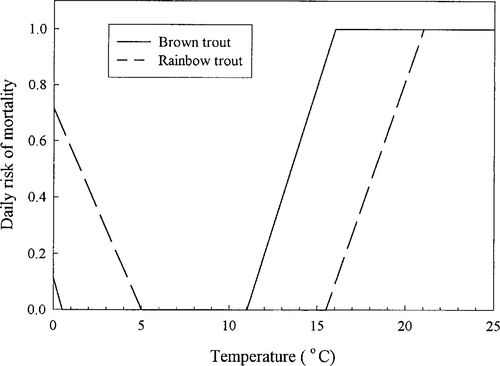
Relationship between simulated redd mortality and temperature for brown and rainbow trout
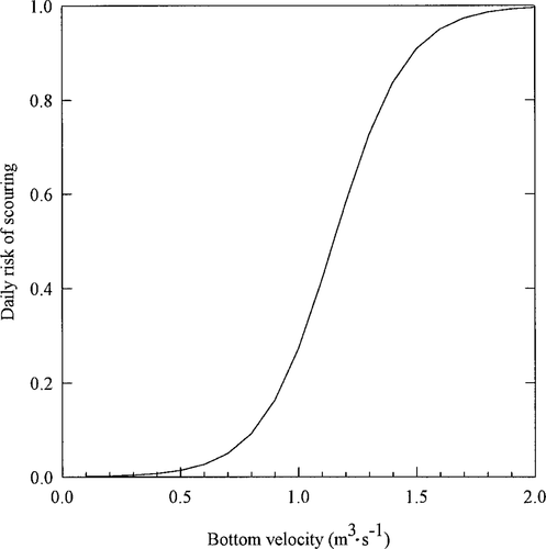
Relationship between simulated risk of scouring and stream bottom velocity for brown and rainbow trout redds
Growth of juvenile and adult life stages
Juvenile and adult life stages are influenced by temperature and flow-driven characteristics of the stream environment in complex ways. Fish growth is optimal at intermediate temperatures (Figure 5) and velocities (Figure 6). The relationships shown in Figure 5 for brown and rainbow trout are intermediate results from the model and not from specified relationships between growth and temperature. The trout model simulates the energetics of individual fish to determine growth as a function of prey intake and energetic costs. Unlike most bioenergetic models, this model does not assume that the trout consumes a fixed percentage of maximum daily consumption. Instead, it calculates the rate of drift intake from (1) the fish's foraging mode (mover versus stayer) (2) the velocity used by the fish while foraging, which is limited by its maximum swim speed (Rand et al. 1993) and surface velocity, (3) the local drift rate (Fausch 1984), and (4) the fish's reactive distance (Hill and Grossman 1993). These relationships in the foraging module are assumed to be the same for both species and are described in Van Winkle et al. (1998). On a daily basis, intake is usually constrained by time available for foraging, but at extreme temperatures the maximum daily intake, Cmax, may be the operating constraint.
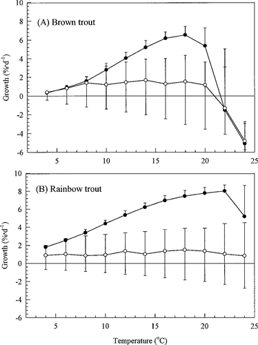
Relationship between growth and temperature for brown and rainbow trout, as predicted by our model for a 70-g trout under maximum (solid symbols) and typical (open symbols) rations. The error bars with typical growth show the range of variation among individual trout in the model. Lower limits of growth with maximum ration are omitted for clarity

Relationship between growth and velocity at different water temperatures for 100-mm long drift-foraging brown trout. This figure was developed from a Mathcad worksheet with equations and parameter values from the population model but without its stochastic features
We started with the assumption that bioenergetic parameters for the two species were not different unless proved otherwise. In two cases, we decided that evidence was sufficient to support species differences. First, we considered differences in the response of Cmax to temperature (Van Winkle et al. 1998) to be significant. Elliott (1976) reported that brown trout ceased feeding at temperatures higher than 21°C, whereas rainbow trout feed at temperatures several degrees higher (From and Rasmussen 1984). Second, the response of standard respiration, Rs, to increased temperature, T, is faster for brown trout (c = 0.0938; Elliott 1976) than for rainbow trout (c = 0.0693; Rao 1968; Stewart 1980). In the following equation, we assumed that parameters associated with trout weight, W, were the same for both species:

Field evidence suggests that the brown trout is the dominant competitor in natural streams where the two species coexist (Gatz et al. 1987). The trout model simulates size-based competition among individuals, giving brown trout a competitive advantage in obtaining a drift-feeding station (Van Winkle et al. 1998). Simulated fish are ranked by a dominance index and allowed to move, forage, etc. in the order of this index. The dominance index for brown trout is 100% of its length, and for rainbow trout, it is 80% of its length. If the drift-feeding stations available in a given habitat unit are all occupied by higher-ranking trout, the lower-ranking individual adopts a “mover” foraging strategy that, we assume, results in a reduced rate of prey intake. The availability of a drift foraging station is calculated for a given trout from the wetted area of a habitat unit and the territory sizes (Grant and Kramer 1990) of dominant prior residents. There is no direct simulation of behavioral occupation or displacement of individuals from specific sites. However, individual trout may be displaced indirectly as the result of a departure rule that causes an individual trout to relocate when the ratio of mortality risk to growth experienced in a particular cell is greater than expected based on its past experience (Jager et al. 1993; Tyler and Rose 1994).
Mortality of juvenile and adult life stages
Susceptibility to two sources of mortality that we simulate depends on the physiological condition and growth of individual trout. In simulations calibrated to historical conditions, mortality was dominated by size-dependent mortality (referred to simply as “predation” in Results), which is meant to represent the effects of starvation, predation, and disease. We used the same relationship, based on Power's (1987) conceptual model, for both species (Van Winkle et al. 1997a). We also simulate starvation directly when the relative weight of a model trout falls below a threshold value of 0.6. In the Results section, we distinguished between deaths that occur in winter and in summer (“winter starvation” and “summer starvation,” respectively).
The model simulates three additional sources of postredd mortality caused directly by environmental conditions. These were not very important to in the simulations reported here and, therefore, did not contribute to differences among climate change scenarios. We simulate (1) stranding, (2) being swept out of the reach by high flows when cover is unavailable, and (3) direct mortality in response to extreme high temperatures. The first two of these are simulated as described in Van Winkle et al. (1998). Simulation of direct temperature-related mortality of trout assumes that mortality risk increases linearly from zero to one as average stream temperature increases from a critical thermal maximum (CTM) to CTM + 2°C. A review of lethal limits reported for both species and all life stages shows that estimates vary widely and seem to be higher in studies conducted in warmer geographic regions. It is commonly believed that brown trout are the most tolerant of high temperature among the trout species, but in many streams, such as the Tule River, brown trout drop out first as temperatures rise downstream (e.g., Kaya 1977; Studley et al. 1996). The regional distributions of the two species with respect to temperatures are similar (Eaton et al. 1995), and at least one laboratory study of thermal tolerance suggests that lethal limits are similar (Lee and Rinne 1980). Because a review of the literature shows very little agreement in settling the question of which species is more tolerant of high temperatures, we assigned the same limit to both species (CTM = 26°C).
Model calibration
Van Winkle et al. (1998) presented the results of extensive model calibration over a 9-year period of record in the reach of the Tule River below the Tule diversion dam. For this study, we added two additional calibration steps to ensure that our temperature relationships adequately represent the situation in the Tule River. First, we compared the relationship between growth and temperature predicted by our model (Figure 5) with that reported for trout species in the literature. At maximum ration, our model predicted a higher peak temperature for growth (16–20°C) than reported, particularly compared with Elliott's (1976) measurement of 12.8°C for brown trout. Despite using Elliott's equations, it was not possible to reproduce his observed growth peak because it is driven to lower temperature by the combined effects of two unmeasured quantities: active respiration and the energy required for digestion and reallocation of stored energy reserves (Figure 9 in Elliott 1976). Other studies have also highlighted the potential importance of and the lack of knowledge about active respiration (Boisclair and Sirois 1993; Qin et al. 1997). Like Elliott (1976), our model predicts a decline in the growth optimum as ration decreases. Trout intake in the Tule River model is so low that it is only constrained by maximum daily intake (Cmax) at extreme temperatures. The response to intermediate temperature in Figure 5 is flat because invertebrate densities in the Tule River are similar year-round (ENTRIX 1993) and because reactive distance responds only weakly to temperature. Streams with more seasonal prey abundances and larger rivers with higher levels of prey (i.e., intake closer to the maximum daily limit) may show a different pattern.
Our second calibration step was to compare historical simulations of an upstream reach above the Tule diversion dam with those of a downstream reach with temperatures that average 3.1°C higher below the confluence with Meadow Creek (Figure 1). The model reproduced the observed historical pattern of decreasing brown trout densities in a downstream direction that was observed in the Tule River. The model predicted extinction of brown trout population in the downstream reach, although four replicate simulations still had a few brown trout alive at the end of the 12 years. Field estimates in the lower reach show much lower brown trout populations than in the upstream reach; on average, 14% of the trout were brown trout in fall population estimates between 1985 and 1992 (Studley et al. 1995: Appendix M). We considered this a reasonable fit because there is evidence that immigration of adults from upstream reaches accounts for a significant fraction of the adult population (Studley et al. 1995). In contrast, 45% of trout remaining in simulations of the upstream reach were brown trout, compared with 52% in field populations (Studley et al. 1995).
Simulation Experiment of Climate Change
We simulated the rainbow and brown trout populations for 12 years with temperatures and streamflows representing historical conditions in the NFMF Tule River, California. We compared historical model results with those produced by temperatures and streamflows representing three climate change scenarios. The scenarios are (1) 2°C increase in average stream temperature, (2) a seasonal shift in streamflow, and (3) the combined effects of a streamflow shift and temperature increase. The following two sections describe our methods for simulating the effects of climate change on stream temperature and flow.
Simulation of Temperature under Historical and Changed Climate Conditions
We developed a stochastic model to simulate average daily temperature for historical conditions in the NFMF Tule River based on temperature records from fall 1985 to fall 1995. We simulated autocorrelated stream temperatures for each day t, T(t), with a sinusoidal function fitted to historical temperatures:

Parameter values fitting historical temperatures were: ω = 0.012, Tdev = 2°C, t0 = day 75, and β = 0.7; Z is drawn at random from a standard normal distribution. For simulations of the upstream reach, T0 = 3°C and Tmax = 15.2°C. For simulations of the warmer downstream reach, T0 = 6°C and Tmax = 20°C.
To simulate climate change effects on stream temperatures experienced by the trout, we simulated a year-round increase in average stream temperatures of 2°C. Several GCM simulations have estimated the change in air temperature in the Sierra Nevada region of California resulting from doubled CO2. Smith and Tirpack (1989) suggested that the increase would be between 1.5 and 5°C. Stamm and Gettelman (1995) predicted that doubling CO2 would produce an average increase of 2°C (range = −1°C to 5°C) in July air temperatures and an average increase of 3°C (range = −1°C to 6°C) in January temperatures. These results were geographically variable, showing the largest increases in the western foothills of the Sierra Nevada. Eaton and Scheller (1996) mapped an average annual increase of about 3.2°C. Because air temperatures are not buffered by groundwater inputs, multiplying by the factor 0.86 (Stefan and Preud'homme 1993) estimates the somewhat smaller change in stream temperature. For all model scenarios with elevated temperatures, we used parameters T0 = 5°C and Tmax = 17.2°C for the upstream reach and T0 = 8°C and Tmax = 22°C in the downstream reach.
We did not attempt to simulate interactions between streamflow and temperature. In reality, stream temperatures usually drop with spring snowmelt, and summer stream temperatures increase when streamflow is low.
Simulation of Streamflow under Historical and Changed Climate
We simulated average daily streamflow for historical conditions by developing a stochastic model fit to historical monitoring data from fall 1985 to fall 1993 in the NFMF Tule River. This record included several wet years, drought years, and normal years, based on snowpack accumulation and total annual flow (J. Grygier, Pacific Gas and Electric Company, personal communication). Generated stream flows, Q(t), came from a date-specific distribution of daily flows observed in the historical record. In the first step we estimated the mean, μ, and variance, σ2, for each date, t. We assumed that the distribution of potential flows on any date is normal: Z is N[μ(t), σ2(t)]. In the second step, we autocorrelated this process by filtering it through a running average with a weighting factor of α = 0.8. We set a minimum flow of 0.17 m3/s. Parameter values for means and variances were selected by fitting to minimize deviations from observed flows over the period of record for each season. The autocorrelation was chosen based on its ability to produce visually similar temporal patterns. The equation below summarizes the stochastic process used to simulate streamflow:

The main hydrologic effect expected to accompany climate change is a shift from snowmelt-dominated high flows in spring to higher winter flows during rain-on-snow events (Lettenmaier and Gan 1990). Our upstream reach is at a transition zone in elevation (1,200–1,300 m) in the western foothills of the Sierra Nevada that is likely to experience high precipitation in the form of rainfall (Soong and Kim 1996). In addition, the watershed draining into the Tule River includes higher elevations that may experience winter rain-on-snow events.
We used hydrologic projections from a Geophysical Fluid Dynamics Laboratory GCM scenario for the Merced River in California to predict streamflow changes under doubled CO2 climatic conditions because these projections were intermediate with respect to the three GCMs evaluated by Lettenmaier and Gan (1990). We selected the Merced River for comparison because it is closest to the Tule River and has a more similar seasonal distribution of flows (i.e., a greater proportion of annual flows occurred in the spring) than do the other three California rivers evaluated by Lettenmaier and Gan (1990).
We estimated Tule River streamflow under doubled CO2 on each day, t, by assuming that the ratio of historical streamflow, QT(t), to that under doubled CO2,Q′T(t), in the Tule River would be the same as the ratio of historical streamflow, QM(t), to streamflow under doubled CO2, Q′M(t), in the Merced River:

The seasonal patterns in flow shift were similar for each of the three GCMs used by Lettenmaier and Gan to project CO2 effects: streamflows were higher in winter and lower during the other seasons. Doubling CO2 shifted the seasonal pattern in streamflow in a simulated 12-year record of streamflow for the Tule River (Figure 7).
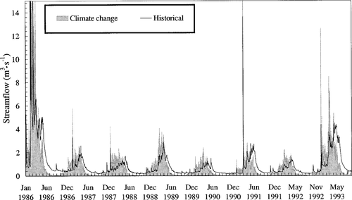
Comparison of seasonal patterns in historical streamflow with simulated streamflow shifted according to the adjustments predicted to occur as a result of CO2-related changes in climate
Simulation Experiment Design
To evaluate potential effects of temperature and flow responses to climate change on the trout populations, we simulated four scenarios in both an upstream and a downstream reach of the Tule River. The four scenarios are (1) the historical flow and temperature regime, (2) historical flow with the mean temperature elevated by 2°C, (3) seasonally shifted flow with historical temperature, and (4) elevated temperature and shifted flow combined. Each simulation consisted of a 12-year period (three to four trout generations). Historical flow, habitat, and population data for the upstream site provided the baseline for all simulation scenarios. Initial abundances, age structure, and size distributions of brown and rainbow trout populations were averaged from estimated population attributes over the period 1986–1992 (Studley et al. 1995) in the upstream reach. Because the model is stochastic, we reported averages from 10 replicate simulations with their standard errors.
We recorded population statistics that allowed us to compare scenarios, including the average number of juvenile and adult trout of each species at the end of September of the last simulated year. We reported the earliest spawning date and the latest date of emergence for each species over the course of 12 simulated years.
One of the advantages of using an individual-based model is that it provides mechanistic explanations for scenario differences. We summarized mortality of fish due to different causes over the 12 years, including both redd and postredd mortality. While these results are valuable, the exact order of importance among the causes of mortality may be influenced by competition among the risks (an increase in one may lead to a decrease in the other) and by uncertainty in parameter values related to mortality (Jager et al. 1997).
Two hypotheses summarize our a priori expectations. In the flow hypothesis, the seasonal shift of peak flows associated with climate change will tend to decrease the incidence of spring floods (during rainbow trout spawning and incubation) and increase the incidence of winter floods (during brown trout incubation). This will cause substantial scouring of brown trout redds and a significant decrease in brown trout population size and a concomitant increase in rainbow trout populations as hypothesized by Strange et al. (1992). Under the temperature hypothesis, the increase in stream temperature will decrease populations of both species because of summer starvation and thermal stress. Because temperatures tend to increase downstream, climate change will restrict the distribution of both species of trout to upstream segments as hypothesized by Keleher and Rahel (1996)
Results
The simulated effects of increased temperature and shifted flow alone and in combination on trout abundances at the end of the 12 years are shown in Figure 8. We interpreted these results by considering changes in mortality caused by each treatment (Figure 9), average final lengths of survivors (Figure 10), and changes in the timing of spawning and incubation (Figure 11). In the following three sections, we present the effects of temperature and flow changes alone, as well as the combined effects of flow and temperature responses to climate change.
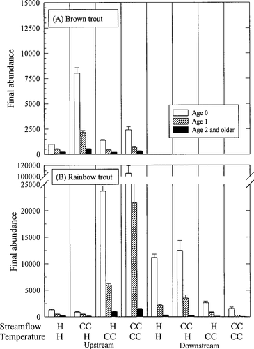
Average abundances of age-0, age-1, and age-2 and older trout on the last day of our 12-year simulations with 1 SE confidence bounds. Results are shown for (A) brown trout and (B) rainbow trout in an upstream and a downstream reach for each scenario. Scenarios are denoted by a temperature and a flow regime (H = historical; CC = climate change)

The percent of total mortality (all life stages) over 12 simulated years represented by each of six mechanistic causes. Each bar represents an average (±SE) over 10 replicate simulations for (A) brown trout and (B) rainbow trout in an upstream and a downstream reach for each scenario. Vertical barred lines are +SE. Scenarios are denoted by a temperature and a flow regime (H = historical; CC = climate change). Causes that did not differ among scenarios are omitted
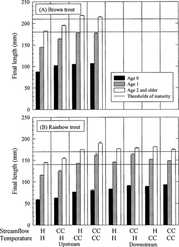
Average (±SE) lengths of age-0, age-1, and age-2 and older trout on the last day of our 12-year simulations with 1 SE confidence bounds. Horizontal reference lines show the minimum size for reproductive maturity and the size at which we assume all adults are mature. Results are shown for (A) brown trout and (B) rainbow trout in an upstream and a downstream reach for each scenario. Scenarios are denoted by a temperature and a flow regime (H = historical; CC = climate change)
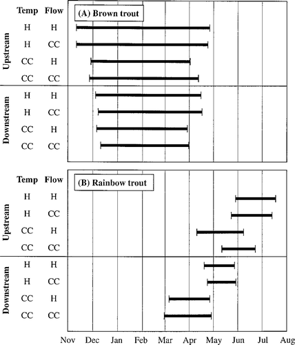
Average over replicate simulations of the earliest spawning date and the latest emergence date during 12 years of simulations, defining the redd incubation period for (A) brown trout and (B) rainbow trout in an upstream and a downstream reach for each scenario. Scenarios are denoted by a temperature and a flow regime (H = historical; CC = climate change).
Climate Change in Streamflow Alone
Shifting high streamflows toward winter had a strong positive effect on brown trout abundance upstream (flow = CC, temp = H in Figure 8A). Rainbow trout populations did not show a large response, but decreased somewhat (flow = CC, temp = H in Figure 8B). This result contrasts with our flow hypothesis. Redd scouring decreased for spring-spawning rainbow trout and increased for winter-spawning brown trout in response to the flow shift as predicted by the flow hypothesis (Figure 9). However, dewatering, which changed in the opposite direction, dominated the overall response to shifted flow. Dewatering posed a greater risk to rainbow trout redds that were constructed at high, shifted flows and later exposed to low flows than the risk posed by scouring at the high flows. Likewise, construction of brown trout redds during lower fall flows was a mitigating factor for dewatering that compensated for scouring events in winter. The shift in streamflow pattern had little impact on spawning and incubation times (Figure 11) but resulted in increased trout sizes in fall (Figure 10).
Climate Change in Temperature Alone
In general, the increase of 2°C in average annual temperature with a historical flow regime increased trout populations in the upstream reach and decreased trout populations in the downstream reach (Figure 8). Brown trout abundance increased slightly in response to elevated temperatures in the upstream reach (flow = H, temp = CC in Figure 8A). In spite of an increased incidence of summer starvation (Figure 9A) in the upstream reach, growth and, thus, fecundity of the survivors was enhanced (Figure 10A). The age structure shifted to a larger proportion of age-0 brown trout.
In the downstream reach, elevated temperatures hastened brown trout extinction through summer starvation of juvenile and adult fish. In simulations with elevated temperatures in the downstream reach, extinction occurred over the first summer, compared with a much slower decline over a period of about 10 years in the historical simulations. The importance of summer starvation (Figure 9A) suggests that energetic conditions were not favorable for brown trout in the downstream reach. In contrast to the upstream reach, there was no growth or fecundity advantage for adults to counteract temperature-related redd mortality and summer starvation of juveniles.
Rainbow trout also increased in the upstream reach and decreased in the downstream reach in response to elevated temperatures (flow = H, temp = CC in Figure 8B). We attribute the increase in rainbow trout in the upstream reach to better growth conditions (Figure 10B) and, therefore, lower predation mortality (Figure 9B). After the first summer of life, rainbow trout in the upstream reach grew faster at the elevated temperatures (Figure 10B). During incubation, the increased temperature caused rainbow trout to spawn earlier (Figure 11B). Redd survival in the upstream reach improved because decreases in redd dewatering more than compensated for increases in scouring that accompanied the shifted incubation period (Figure 9B). Even with the extended spawning period, earlier spawning by rainbow trout caused most fry to emerge from the redds before summer low flows (Figure 7).
Downstream, we attribute the decline in rainbow trout to increases in the incidence of (1) redd mortality due to extreme incubation temperatures and (2) summer starvation, when compared with the historical simulations (Figure 9B). The increased duration of the incubation period increases background redd mortality (not shown in Figure 9B, but see Figure 11B). However, the surviving rainbow trout grew faster in the downstream reach (Figure 10B).
Temperature had significant effects on the timing of spawning and incubation. Spawning for brown trout was delayed by several weeks because lower temperatures required to spawn did not occur until later in fall (Figure 11A). Brown trout eggs and alevins developed faster and fry emerged considerably earlier under the climate change scenarios with elevated temperature. The onset of rainbow trout spawning shifted to an earlier date, particularly downstream. This extended the duration of the incubation period for rainbow trout in the downstream reach (Figure 11B).
Combined Effects of Streamflow and Temperature
The effects of streamflow and temperature were not additive. In Figure 8, it does not appear that final population abundances of the combined scenario can be predicted by a linear combination of the final abundances from simulations changing each factor alone. One clear example in these simulations was the tremendous increase in rainbow trout abundance upstream when both temperature and flow effects were simulated (flow = CC, temp = CC in Figure 8B). Rainbow trout grew faster in both the temperature (flow = H, temp = CC) and the flow (flow = CC, temp = H) scenarios than they did under historical conditions (flow = H, temp = H in Figure 10B). The two climate changes together caused even faster growth and caused age-1 rainbow trout in the upstream reach to pass a threshold size, enabling the majority to reach reproductive maturity at least 1 year early. Although the effects on average growth may be additive, the population-level effects caused by this shift in life history were much greater than would be predicted by extrapolating from temperature effects on growth alone.
Another interaction effect occurred when elevated temperatures shifted the timing of spawning and incubation, exposing redds to a seasonally shifted flow regime. Brown trout redds experienced more scouring with both flow and temperature changes in climate because they were constructed later and at higher winter flows (Figure 9A). As a result, no decrease in dewatering compensated for scouring mortality of brown trout redds when we simulated combined effects of flow and temperature.
Discussion
These simulations revealed that changes in hydrology can play an important role in mediating climate change effects on trout. Important nonadditive interactions between hydrologic and temperature effects were produced by changes in the juxtaposition of the incubation period with flow-related disturbances. Simulation results suggested that changes in dewatering mortality, as well as scouring mortality, must be understood to predict the consequences of hydrologic shifts. This experiment raised the possibility of nonlinear threshold population responses resulting from the combined effects of the two climatic factors (e.g., faster rainbow trout growth shifted the age at first maturity). Finally, our results were consistent with the habitat fragmentation hypothesis proposed by Keleher and Rahel (1996) and Rahel et al. (1996). Simulation results suggest that thermal effects under climate change regimes predicted for the Sierra Nevada would reduce brown and rainbow trout densities in downstream reaches of the Tule River and similar rivers.
The specific model predictions of abundance presented here depend on a fairly large number of assumptions and parameter estimates, and we do not know if they are quantitatively reliable. However, we have faith in the qualitative patterns produced by the two climatic variables because, in hindsight, they are intuitively reasonable. In the discussion of the patterns that we expected ahead of time (our flow and temperature hypotheses below), it is clear that we did not anticipate all of the climate change effects that were predicted, particularly those involving both climatic factors. These unexpected patterns could not easily have been predicted a priori without the help of a model to reveal the implications of the complex processes involved.
Temperature Hypothesis
Our temperature hypothesis was that summer starvation and high temperature mortality would be a critical problem for both species. The simulated effects of elevated temperature reported here supported the first part of the hypothesis: that summer starvation would be a problem, particularly for brown trout. Direct mortality caused by lethal, high temperatures did not occur in the simulations. Although there is some field evidence suggesting that trout prefer high, but sublethal temperatures (Matthews et al. 1994), the relative importance of starvation and exposure to lethal temperature may depend on site-specific prey availability. It has been suggested that increased prey levels may permit brown trout to inhabit warmer reaches (Preall and Ringler 1989). In addition to starvation, redd mortality at high temperatures was an important source of mortality. Even with increased levels of prey, our results suggest that elevated incubation temperatures would still be a problem for trout, unless redds were located in areas moderated by groundwater inflow or farther upstream. To explore this a bit further, we simulated brown trout alone in the downstream segment under historical conditions, but with a higher rate of drifting prey. The results showed that increasing prey did slow the decline of the simulated brown trout population, but it did not lead to persistence, despite a very fast growth rate for survivors.
Streamflow Hypothesis
Our flow hypothesis was that increased scouring of brown trout redds rather than rainbow trout redds would result from shifting high flows from spring to winter. Model results reflected this, but final abundances were more influenced by other factors besides scouring. Even though our hypothesis about scouring held true, the total effect of flow on brown trout was opposite of what we expected, based solely on scouring. One result that emerged from this simulation study is the hypothesis that dewatering of redds in the spring may be an important factor to consider in evaluating hydrologic climate change effects.
Future Directions
It is unclear at this point whether these results generalize to other streams in the Sierra Nevada. Only comparison with longitudinal patterns in other streams can address this question. This study raises questions about the relative temperature tolerance of the two trout species and whether prey availability or interannual variation in flow mediate the competitive outcome. These questions can be addressed by field experimentation, regional analysis, and improved measurement of thermal and flow responses of trout species (especially activity costs of older fish and redd mortality).
The role of spatial heterogeneity in predicting effects of climate change on trout is unclear. At a larger spatial scale, effects of habitat fragmentation by physical and thermal barriers can be evaluated. In addition to the effects of reduced habitat, the extinction risk of small, isolated populations is generally higher than that of larger, interconnected ones. At a smaller spatial scale, there is a need for statistical models of within-reach spatial variation in stream temperature to quantify mitigating effects of thermal refuges. Nielsen et al. (1994) described the importance of thermal refuges for steelhead (anadromous rainbow trout) in northern California streams. They suggested that thermal refuges are created by barriers to thermal mixing (e.g., woody debris, deep backwater pools, significant tributary inflows, and intergravel flow). Groundwater temperatures also influence local stream temperatures and, in particular, trout incubation (Meisner 1990). Likewise, the spatial distribution of flow effects, as mediated by the availability of cover and redd depth, is incompletely understood.
Another aspect that we did not explore in this study is the potential for an evolutionary response to climate change. It has been suggested that California's rainbow trout populations have higher thermal tolerance than those farther north (Matthews et al. 1994). It would be interesting to determine whether this geographic variation has a genetic basis. Traits such as thermal tolerance, growth, maturation, and spawning time are potentially relevant. Trade-offs may exist between thermal tolerance and growth efficiency, as found by Redding and Schreck (1979) between coastal and inland steelhead populations. Maturation cues and thermal tolerances of the egg life stage may also be important traits. Kaya (1977) found that brown trout in a geothermal stream showed abnormal gonadal maturation in a high-temperature site. In contrast, rainbow trout responded behaviorally by shifting from spring to fall spawning. Spawning time is influenced by environmental factors (temperature and photoperiod), but also shows strong maternal heritability (Danzmann et al. 1994). Individual-based models would be ideally suited to organizing available data on heritability of and correlations among relevant traits and pursuing the long-term implications of gradual climate change.
Acknowledgments
The Pacific Gas and Electric Company staff, especially Tom Studley, were very helpful in providing us with field data from the Response of Fish Populations to Altered Flows Project. We appreciate partial support provided by the Southern California Edison Company through Tailored Collaboration with the Electric Power Research Institute. The Electric Power Research Institute supported this research under contracts DOE ERD-94-1220 (WO2932-2) and ERD-95-1341 (WO9111-02) with the U.S. Department of Energy. Oak Ridge National Laboratory is managed by Lockheed Martin Energy Research Corp. for the U.S. Department of Energy under contract DE-AC05-96OR22464. Thanks are due Chuck Coutant, Richard Strange, Joe Cech, and Chris Myrick for sharing information on the relative thermal tolerances of brown and rainbow trout. We appreciate excellent reviews provided by S. F. Railsback, R. M. Cushman, P. J. Mulholland, J. J. Magnuson and two anonymous reviewers. This is publication 4738 of the Environmental Sciences Division.
Appendix: Simulation of Stream Habitat
Depth (D) is estimated for each model cell using a stage–discharge relationship as is done in the IFG4 component of PHABSIM:

where Di(0) is the depth of water in cell i at zero flow (Q = 0). The parameters of this relationship are estimated by PHABSIM for each transect, along with the bottom elevation of each cell, and provided as input to the trout model.
The method used to estimate velocity for each donor cell depends on the calibration data available for the cell. Three methods are (1) the power equation, (2) Manning's equation, and (3) the high-flow method. For cells with hydraulic data for three or more calibration flows, a power relationship can be developed, and used to estimate velocity (V̂) from flow (Q):

For cells with velocity measurements (i.e., those that were inundated) for fewer than two calibration flows, Manning's equation is used with PHABSIM estimates of the roughness coefficient (n) at each calibration flow and depth (D). Each habitat unit lacking slope information was assigned a slope (S) from a range specific to its mesohabitat type.

Manning's equation is also used to estimate velocity in situations when the power equation estimates are unreasonable (i.e., the estimated velocity is negative or exceeds a specified maximum velocity of 2.5 m/s). For cells that lack estimates of hydraulic parameters because depths were too shallow to allow velocity to be measured, we estimate the roughness from roughness estimates for a neighboring cell and from estimates at other calibration flows. For example, assume that no estimate of roughness is available for cell i at the low calibration flow (Ni,low). We estimate Ni,low from roughness estimates for an adjacent cell, j, and the roughness at a higher calibration flow as

For very high streamflows (above bank-full), we assume that the IFG4 parameter estimates (n, c, and d) are no longer accurate, and we use the high-flow method (Manning's equation with different parameter values for slope and roughness). Because the distinctions among mesohabitat types tend to blur at higher flows, we assume that all habitat types have converged to the same water surface slope (the average for the reach) and that all roughness parameters have decreased to a specified minimum value that is calibrated to produce high, but reasonable, velocities.


