The Effects of Age-0 Body Size on the Predictive Ability of a Largemouth Bass Bioenergetics Model
Present address: Arizona Game and Fish Department, Research Branch, 2221 West Greenway Road, Phoenix, Arizona 85023, USA.
Abstract
Bioenergetics models for largemouth bass Micropterus salmoides have provided scientists with a valuable tool for estimating growth and consumption based on temperature and the size of individuals. These models were developed for a wide range of fish sizes from various geographic origins and have been used to generate predictions for fish across the entire size and geographic ranges of largemouth bass. Although previous studies have shown general validity in model predictions, no validation has been achieved for smaller-bodied largemouth bass from differing geographic populations. To test the accuracy of a commonly used model at predicting the growth of small largemouth bass, we ran a series of six 14-d aquarium experiments that included controlled feeding rates over the range of average daily water temperature regimes in central Alabama. Age-0 largemouth bass from one population in Wisconsin (northern largemouth bass M. s. salmoides) and two populations in Alabama (Florida largemouth bass M. s. floridanus and northern largemouth bass) were fed at two ration levels, and the actual amount consumed over the 14 d was used to predict growth, which was compared with observed growth. Survival was similar among populations and decreased at higher temperatures. The bioenergetics model inaccurately predicted the growth of age-0 largemouth bass for all three populations. The bias associated with model predictions increased with temperature. Additionally, model predictions were more accurate for the Florida subspecies than for the northern subspecies throughout the temperature ranges covered in our experiments. These results suggest that differences in body size and source population may influence the relative accuracy of growth predictions by the current model. Refinement of bioenergetics model parameters to more accurately represent the physiology of smaller individuals across the broad latitudinal range of largemouth bass is necessary to allow better predictive ability of growth in age-0 largemouth bass populations.
Introduction
Bioenergetics models have provided a valuable tool for understanding relationships among temperature, consumption, and physiology of aquatic organisms. These models have rarely been tested against real-world data, and the rate at which bioenergetics models are evolving is far greater than the rate at which their accuracy has been evaluated (Ney 1993). In addition, the parameters in bioenergetics models reflect physiological mechanisms subject to selective pressure that can occur as a function of environmental gradients.
The most widely used bioenergetics model for largemouth bass Micropterus salmoides was originally described by Rice et el. (1983) and was based on parameters borrowed from the literature or estimated from field observations. Caloric densities of largemouth bass used in the original model creation were estimated from largemouth bass (>150 g) from Tennessee (Adams et al. 1982). Maximum consumption and its computational components were estimated from largemouth bass weighing 115 ± 20 g (mean ± SD) from Ontario (Niimi and Beamish 1974). Physiological parameters—such as respiration (estimated from 40−400-g fish from Ontario; Rice 1981, as derived from Beamish 1970), specific dynamic action (estimated from 64 ± 48.5-g fish from Ontario; Beamish 1974), and egestion and excretion rates (estimated from 64 ± 48.5-g fish from Ontario; Beamish 1972, 1974; Niimi and Beamish 1974)—were also based on data collected for largemouth bass of varying sizes and from several geographically distinct populations. Growth data used in model generation were developed from more than 2,200 largemouth bass sampled from a population in South Carolina ranging in weight from 50 to 1,800 g (Rice et al. 1983). Given the diversity of sources of these input data, there is an inherent assumption that the model accurately depicts largemouth bass growth and consumption across a wide range of sizes and geographic locales.
Preliminary evaluations of bioenergetic model parameters for largemouth bass have shown general validity in model predictions for individual populations of larger-bodied individuals. In one of the first rigorous evaluations, Rice and Cochran (1984) tested the validity of the largemouth bass bioenergetics parameters established by Rice et al. (1983) as applied to age-3 largemouth bass from Minnesota (weighing an average of 129 g initially; Cochran and Adelman 1982). In their tests, these size data were compared with sizes predicted by the bioenergetics model, and they found that body masses predicted by the model were within the 95% confidence interval surrounding the observed growth pattern. Further, they employed a series of statistical tests to determine lack of fit, partitioned mean squared error, and internal reliability of their results. These statistical tests showed no significant lack of fit associated with the model, 76% of the error present was due to random chance, and the predicted masses were within 89.28% (reliability index k = 1.12) of the observed masses. This validation itself has fallen under question because of the lack of model fit when only considering initial and final weights and the representation of activity at a constant swimming speed (Ney 1993). Additionally, the Rice and Cochran (1984) validation only implies a good fit for predictions of age-3 largemouth bass consumption within the size range tested.
Whitledge and Hayward (1997) conducted a laboratory experiment with adult largemouth bass (mean initial weight, ∼178 g) from central Missouri to further evaluate bioenergetics model predictions and similarly used a three-step statistical process to validate the model. The first test consisted of a multivariate profile analysis that yielded no significant differences between model predictions and measured masses. The second procedure, comparable to Rice and Cochran (1984), partitioned three sources of mean squared error and found that 87% of the error associated with the model predictions was due to random chance and 6% and 7% were attributable to mean and slope difference, respectively. Finally, they calculated a reliability index (k; Rice and Cochran 1984; Wahl and Stein 1991) and determined that 68% of the predicted weights would fall between 0.97 and 1.03 times the predicted weights. Again, this validation was conducted for adult largemouth bass, but no initial size range and age were presented.
Though these evaluations have shown the model to be valid for single populations of larger-sized individuals, no validation has been achieved for age-0 largemouth bass of similar sizes from different geographic sources. Herein, we quantify growth and survival of age-0 largemouth bass from three origins (Wisconsin, central Alabama, and southwest Alabama) for comparison with bioenergetics model predictions. Model predictions were compared with observed weights from a series of controlled experiments to determine whether the current model accurately predicted growth of age-0 largemouth bass. Statistical analyses similar to those of Rice and Cochran (1984) and Whitledge and Hayward (1997) were used to test for bias in the bioenergetics model predictions based on initial size and geographic source population and to facilitate comparisons with previous validation efforts.
Methods
Origin of experimental fish
Adult largemouth bass from three geographically distinct populations were brought to Auburn University during the winter of both 1998–1999 and 1999–2000. These populations were inhabitants of south-central Wisconsin (Wisconsin population; 43°N), the Mobile River delta near Spanish Fort, Alabama (Delta population; 30.5°N), and experimental ponds at Auburn University (Florida population; 32.5°N but originally native to peninsular Florida [28°N]). Genetics tests confirmed the subspecies of each population (Slaughter 2002); the Wisconsin and Delta populations were northern largemouth bass M. s. salmoides, and the Florida population was Florida largemouth bass M. s. floridanus. These adults were stocked (20 fish/pond) into two 0.04-ha spawning ponds per population. Fathead minnow Pimephales promelas were added (approximately 250 kg/ha) once per month to provide prey to these ponds. Spawning by largemouth bass took place in early spring both 1999 and 2000. The progeny produced by these spawns were used as our experimental subjects.
Experimental design
From July 1999 through August 2000 we conducted six laboratory feeding trials on individual age-0 largemouth bass at different temperatures. Trials consisted of placing a single fish in each of 30-L to 60-L aquaria (10 fish per population) and feeding them a controlled ration (see below) once per day for 14 d. Aquaria were housed in a room with controlled photoperiod (set to correspond with local conditions); temperatures were allowed to fluctuate with local temperatures. Temperature data loggers (Onset Computer Corporation, Optic StowAway Tidbit model) were placed into two aquaria (selected at random) and recorded at 1-h intervals throughout each feeding trial. These trials were run at varying temperatures covering the entire temperature range for central Alabama (12–32°C; Slaughter 2002).
Aquarium sampling
Age-0 largemouth bass from each population (45–193 mm total length; weights varied with time; see Results) were randomly collected from the spawning ponds via beach seine at least 2 d before the start of each feeding trial, placed individually into 60-L aquaria, and acclimated for 48 h. An additional random subsample of 10 bass from each of the three populations was taken from the spawning ponds to quantify initial caloric density. On the first day of each trial, each fish was removed from its tank and weighed (wet weight; nearest 0.1 g) and measured (total length; nearest 1 mm) to predict its maintenance feeding ration. At the end of the 14-d period, fish were weighed and measured, and their caloric was density determined.
Daily feeding rations
Two ration levels were used in our experiments, such that five replicate fish from each population received the maintenance ration and five received a 1.5× maintenance ration. Based on the initial weight of each fish, maintenance feeding rations were calculated to yield no gain in weight using the Fish Bioenergetics 3.0 model (Hanson et al. 1997) and predicting consumption over the 14-d period at anticipated water temperatures and estimated caloric densities for predator and prey. Prey used in the experiment consisted of 15–35-mm western mosquitofish Gambusia affinis or guppies Poecilia reticulata. Caloric density of prey fish was determined via bomb calorimetry during each experiment (see below).
Caloric densities
Each sample (either individual largemouth bass or prey fish) was weighed and placed in a 60°C drying oven until the change in sample weight on consecutive days was less than 0.01 g. Once dry, the sample was pulverized into an homogeneous mixture and returned to the drying oven until consecutive daily weights changed by less than 0.01 g. Dried, ground samples were then pelleted and ignited in a bomb calorimeter (Parr, Model 1425, semi-micro bomb calorimeter) to measure caloric content (cal/g). Bomb calibration with benzoic acid standards took place at 200-run intervals, though very little drift in bomb measurements occurred. When sufficient tissue was available, replicate samples from each fish were ignited until two caloric densities were within 2% of one another. The caloric density for each fish was then determined as the average of all caloric measurements for that sample. Approximately 90% of samples measured had caloric densities within 2% after two bomb runs, and no samples required more than four runs.
Bioenergetics modeling
Final weight was predicted for each experimental fish (based on temperature, total daily consumption, initial weight, and initial and final caloric density as measured during each experiment) by implementing a modification of the current bioenergetics model that predicts final weight from total daily consumption (Wright 1993). Temperature was input as average daily water temperature. Daily consumption was input as the total weight of prey consumed in the 24-h interval between feedings across all 14 of the 24-h feeding periods. Initial caloric density was estimated using linear regression for caloric density by wet weight calculated from the initial subsample for each treatment during each experiment. Final caloric density was input as the amount of calories measured for each individual fish. Model output was the predicted final weight for each fish, which was compared with the observed final weight.
Statistical analyses
Survival was related to temperature and initial weight via nonlinear regression. Significance was set at α = 0.05 for all statistical tests except the comparison of survival to temperature, which was set at α = 0.10 owing to small sample size (n = 6).
Specific growth and consumption rates were calculated for each largemouth bass in each experiment for comparison with temperature and initial weight. Specific growth rate (SGR) was calculated as the change in weight (g) divided by the initial weight (g) divided by the number of days (d). Specific consumption rate (SCR) was calculated as the total weight of food consumed in the experiment (g) divided by the initial weight of the fish (g) divided by the number of days (d). The SCR was not segregated by ration level because experimental fish haphazardly consumed prey items independent of ration level. The SGR was then compared with SCR via least-squares linear regression for each population at each temperature, and an energetic efficiency term was calculated by dividing SGR by SCR for each individual bass for comparisons among populations across temperatures and sizes.
A multivariate profile analysis (Whitledge and Hayward 1997; Hair et al. 1998) was used to compare predicted and observed final weights for each population based on temperature and initial wet weight. Hotelling's T2 was used to identify significant differences between observed and predicted values. This statistical analysis, similar to a t-test, tested the null hypothesis that the trajectories of the predicted and observed values were parallel with a difference in intercept of zero (Whitledge and Hayward 1997).
For each fish in each experiment, a bias term was calculated by taking the difference between the observed and predicted final weights and dividing by the observed final weight. This bias term represented the proportion of observed weight unaccounted for by the weight predicted by the bioenergetics model. This bias term for each fish was compared with mean water temperature for that experiment and initial weight for each bass via least-squares linear or nonlinear regression to produce a predictive model of bias based on temperature and initial weight for each latitudinal population. Additionally multiple linear regression was used to predict model bias by both mean experimental temperature and initial weight.
Additionally, two procedures described by Rice and Cochran (1984) were used to evaluate trends in the model error. A validation procedure (Rice and Cochran 1984; Wahl and Stein 1991; Whitledge and Hayward 1997) was used to describe trends in model error for each latitudinal population and each temperature period. This validation procedure partitions the mean squared error for each temperature and population into three component sources of error. The equation used in the calculation of this mean squared error (MSE) is

where P̄ and Ā represent the mean predicted and actual weights, SP and SA represent the standard deviations of the mean predicted and actual weights, and r is the correlation coefficient of the least squares linear regression of predicted versus actual weights (Mincer and Zarnowitz 1969; Lisson et al. 2000).
By dividing equation (1) by the resulting MSE term, the proportion of the error attributable to the three component sources of error was described (Rice and Cochran 1984):

The mean component (MC) described the error resulting from differences in the mean predicted and actual weights. The slope component (SC) described the error resulting from deviation of the slope (of the regression of predicted and observed weights) from unity (1:1). The residual component (RC) described the random error held within the MSE term.
The final statistical evaluation employed was the reliability index k (originally described by Leggett and Williams 1981; used by Rice and Cochran 1984; Wahl and Stein 1991; Whitledge and Hayward 1997). The following equation was used to calculate k for each latitudinal population at each temperature:

where N is the number of fish from each population at each temperature, yi is the observed weight, and xi is the predicted weight (Leggett and Williams 1981). The resulting k value provided information that 68% of the observed weights are expected to lie between 1/k and k times the predicted weights (Leggett and Williams 1981; Rice and Cochran 1984).
Results
Age-0 largemouth bass body sizes and survival rates were similar among populations across all temperatures. Bass available for feeding trials were generally smaller during warmer periods (i.e., summer) than during cooler periods (i.e., late fall and winter; Figure 1), whereas survival was similar among populations. Although there were no significant differences in initial wet weight among populations across all temperatures, the Florida population was significantly heavier than both the Wisconsin and Delta populations (both P < 0.01) during the 14°C experiment. Furthermore, survival decreased with increasing temperature for the Wisconsin (nonlinear regression; P = 0.018) and Florida (nonlinear regression; P = 0.083) populations, but no significant effects were noted for the Delta population (P = 0.95). Additionally, initial weight was not found to influence survival because all nonlinear regressions were insignificant at α = 0.05 (all P > 0.11).
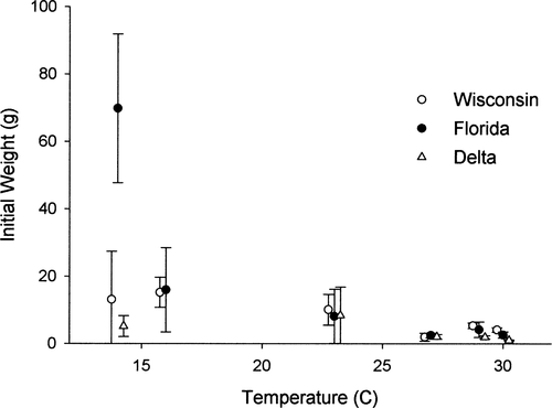
Mean initial weight (±1 SD) as a function of the mean water temperature, by trial, for largemouth bass from three latitudinally distinct populations (Florida, Wisconsin, and Delta) that were used in controlled feeding trials
Growth
Specific growth rates (SGR) increased significantly with temperature for both Wisconsin (P = 0.004, r2 = 0.90) and Florida (P = 0.014, r2 = 0.81) populations. The SGR also increased with temperature for the Delta population, although this relationship was not statistically significant (P = 0.15, r2 = 0.55). Overall, mean SGR across all sizes and temperatures was greatest for the Delta population (3.389 ± 2.024 g/g/d [mean ± SD]) followed by the Wisconsin (2.358 ± 1.473 g/g/d) and Florida populations (2.341 ± 1.744 g/g/d). Initial weight and SGR were negatively correlated for all three populations (all P < 0.01).
Specific consumption rate (SCR) decreased with increasing temperature for both Wisconsin (P = 0.002, r2 = 0.922) and Florida (P = 0.005, r2 = 0.885) populations but was not significantly related to temperature for the Delta population (P = 0.105, r2 = 0.637). The SCR decreased as initial weight increased (all P < 0.002, all r2>0.21) for all populations. Further, SCR was unaffected by daily feeding ration because fish did not consistently consume all prey items available to them during each feeding period; therefore, no segregation based on ration level was made among individuals or specific growth rates.
The SGR also was significantly related to SCR for all three populations (r2 ≥ 0.88, P < 0.001, N = 45–53). The slope of this relationship served as an indicator of the efficiency at which individuals from these populations converted their food to body weight. It is important to note that although these overall relationships were highly correlated (r2 > 0.87, P < 0.001), several factors affect the energetic efficiency of these organisms (namely, temperature and body size) such that the slopes of the regression of SGR to SCR broken down by temperature provide evidence of differences in the growth efficiency among populations (Figure 2). Analysis of covariance (ANCOVA) showed that significant differences did exist among slopes of the SGR versus SCR relationship among populations (F = 31.163; df = 1, 104; P < 0.001), where the Wisconsin population converted consumption to growth at the highest rate, followed by the Florida and the Delta populations (Figure 2).

Specific growth rate (g/g/d) as a function of specific consumption rate (g/g/d) for three latitudinally distinct populations of largemouth bass (Florida, Wisconsin, and Delta) as a function of mean water temperature for each feeding trial. Panel legends show symbols for the mean water temperatures (°C). Regression lines are plotted for each population independent of temperature
There were significant decreasing trends in the energetic efficiency of the three populations with increasing mean water temperature (Figure 3). Conversely, energetic efficiency was positively correlated with initial wet weight for both the Florida and Delta populations, yet remained relatively constant for the Wisconsin population (Figure 3). There were significant differences among populations in energetic efficiency across temperatures (ANCOVA: F = 9.167; df = 1, 5; P < 0.001), but there were no detectable differences among populations related to initial weight (F = 0.931; df = 1, 125; P < 0.614).
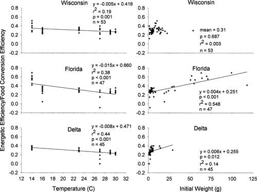
Energetic efficiency as a function of mean water temperature (left-hand panels) and initial weight (right-hand panels) for three latitudinally distinct populations of largemouth bass (Florida, Wisconsin, and Delta)
Model Testing
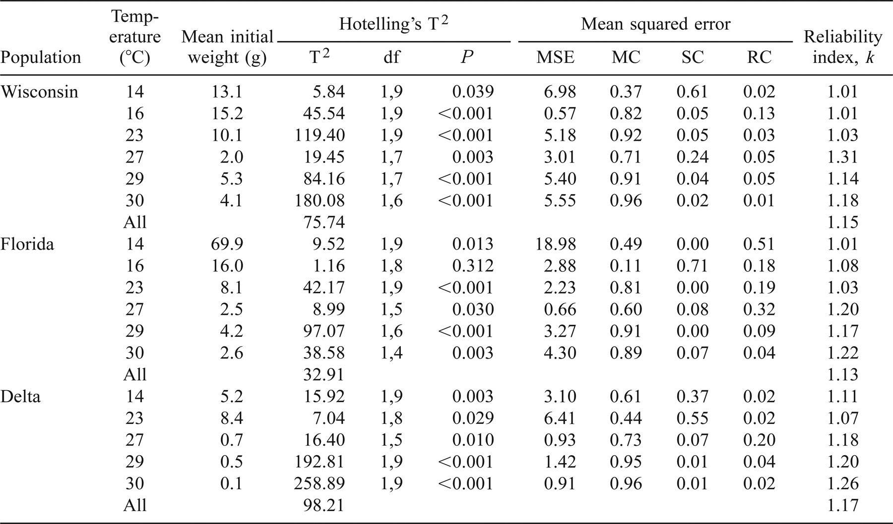
Multivariate profile analysis indicated that model predictions differed significantly from observed weights for all populations at all temperatures except for the Florida population at 16°C (Table 1). Further, the Hotelling's T2 statistic increased exponentially with temperature for each population (Figure 4) indicating increased model bias at smaller body sizes. The most pronounced increase in the T2 statistic was for the Delta population, followed closely by the Wisconsin population. The Florida population, although showing some increase with temperature, increased less than the other two populations. The T2 values did not differ significantly among populations (ANCOVA: F = 2.445, P = 0.101), although this relationship was nearly significant. Further, the Hotelling's T2 statistic showed no significant correlation with initial weight for any of the three experimental populations (r2 ≥ 0.49, P ≥ 0.187).
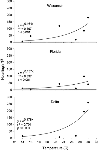
Nonlinear regressions of Hotelling's T2 statistic and mean water temperature for three latitudinally distinct populations of largemouth bass (Florida, Wisconsin, and Delta).
The model consistently underpredicted growth for all three populations in all but one experiment. Model bias was significantly different among populations across temperatures (ANCOVA: F = 34.906, df = 1, 138; P < 0.001) and initial weights (ANCOVA: F = 2.173; df = 1, 125; P = 0.030). The bias was positively correlated with temperature and negatively correlated with initial wet weight for each population (Figure 5). Using simple multiple regression, the following equations were generated to predict model bias based on mean water temperature (T) and initial wet weight (Wini):
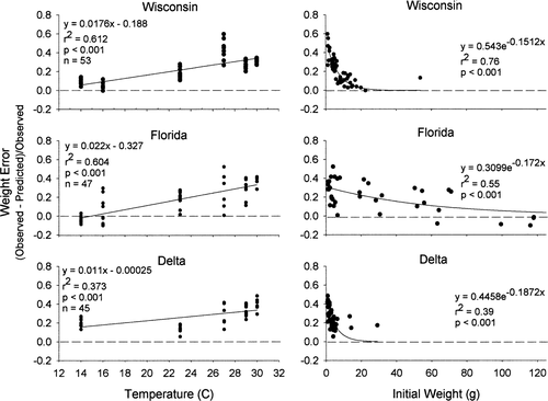
Bias in bioenergetics model predictions of weight as a function of mean water temperature (left-hand panels) and initial weight (right-hand panels) for the three latitudinally distinct populations of largemouth bass (Florida, Wisconsin, and Delta).
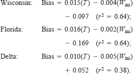
All regressions were significant at P < 0.001. Mean error also increased with increased SGR for all three populations, though only the Wisconsin and Florida regressions were significant at α = 0.05.
Additional analysis of model error was made by comparing predicted with actual weights for the experimental subjects (Figure 6). The slopes of the least-squares linear regressions of predicted and actual weights showed that the model, on average, underpredicted final weight for the Wisconsin (slope = 0.93) and Delta (slope = 0.84) populations and overpredicted weight for the Florida population (slope = 1.05).
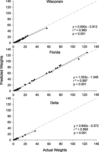
Predicted final weight as a function of observed final weight for individuals from three latitudinally distinct populations of largemouth bass (Florida, Wisconsin, and Delta). The slope component of the mean squared error (MSE) calculation is based on the deviation of the regression coefficient of predicted on observed values from unity (dashed line). Additionally, the r-value from each regression is used in the calculation of both the slope component and the portion of MSE due to random chance.
Table 1 shows the results of the mean squared error (MSE) analysis broken down by population, mean water temperature, and mean wet weight. The MSE was, on average, 4.45, 5.39, and 2.55 for the Wisconsin, Florida, and Delta populations, respectively. These MSE terms showed substantial error in all but one trial for both the Wisconsin and Florida populations and in three of the five feeding trials for the Delta population. For the Wisconsin, Florida, and Delta populations, respectively, the mean component (MC) error term averaged 0.78, 0.64, and 0.74; the slope component (SC; Figure 6) averaged 0.17, 0.14, and 0.20; and the portion of MSE due to random error (RC) was 0.05, 0.22, and 0.06. No trends were detectable among MSE or its component terms when compared with temperature.
The MSE was not related to initial weight for the Wisconsin population (P = 0.717, r2 = 0.04), but it increased significantly with initial wet weight for the Florida (P = 0.002, r2 = 0.94) and Delta (P = 0.003, r2 = 0.97) populations. The MC generally decreased as initial wet weight increased, but the relationship was significant only for the Delta population (P = 0.019, r2 = 0.88). The SC remained constant across initial wet weights for the Wisconsin and Florida populations (P > 0.601, r2 < 0.07) and increased significantly for the Delta population (P = 0.002, r2 = 0.98) with increased initial wet weight. The random component (RC) remained constant for both Wisconsin and Delta populations (P > 0.367, r2 < 0.21) and increased with initial wet weight for the Florida population (P = 0.043, r2 = 0.68).
We used step-wise multiple regression analysis to show trends in MSE and its components based on the combined interaction of temperature and initial wet weight. The MSE was significantly correlated with the combined effects of temperature and initial weight for both the Florida (P = 0.002, r2 = 0.99) and Delta (P = 0.011, r2 = 0.99) populations, but no significant correlation was found for the Wisconsin population (P = 0.943, r2 = 0.04). The MC was significantly related to initial weight and temperature for the Wisconsin population (P = 0.040, r2 = 0.88) and was marginally significant for the Florida and Delta populations (P = 0.095, r2 = 0.79 and P = 0.109, r2 = 0.89, respectively). SC was significantly related to temperature and initial weight for the Delta population (P = 0.011, r2 = 0.99) and was marginally significant for the Wisconsin (P = 0.093, r2 = 0.79) and Florida (P = 0.152, r2 = 0.72) populations. The RC was not correlated with temperature and initial weight for any of the three populations (P > 0.2, r2 < 0.68).
The reliability coefficient k increased significantly with mean water temperature for the Florida population, was approaching significance for the Wisconsin population, and was not significantly correlated with temperature for the Delta population (Table 1; Figure 7). The coefficient decreased exponentially with increased wet weight for all three populations. Also, k was significantly related to the combined effects of temperature and initial wet weight for the Wisconsin population (P = 0.022, r2 = 0.92), was marginally significant for the Florida population (P = 0.151, r2 = 0.72), and was not significant for the Delta population (P = 0.809, r2 = 0.19). The relationships of k to temperature was also found to differ significantly among populations (F = 6.272; df = 1, 5; P = 0.006).
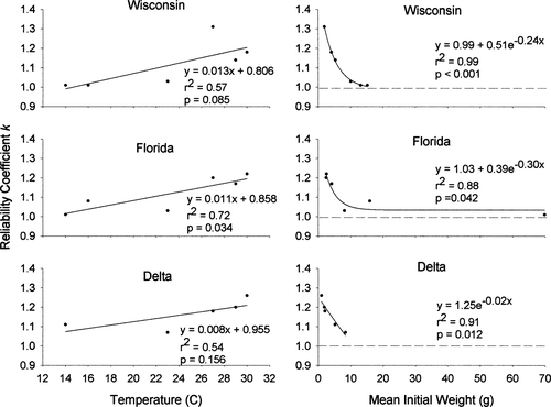
Reliability coefficient (k, which is based on the comparison of observed final weight and the final weight predicted by the bioenergetics model) as a function of mean water temperature (left-hand panels) and initial weight (right-hand panels) for three latitudinally distinct populations of largemouth bass (Florida, Wisconsin, and Delta). In the right-hand panels, the dashed line at k = 1 represents absolute reliability of predicted weights.
Discussion
During our 14-d trials, we found differences in the survival and growth of age-0 largemouth bass across three latitudinally distinct populations. In addition, we found that the largemouth bass bioenergetics model provided inaccurate predictions of growth, bias differing across populations and increasing with temperature and decreasing with increased size. Below we further examine these results in the context of this widely distributed species.
Survival
Survival generally was lower for both the Wisconsin and Florida populations at warmer temperatures than for the Delta population, as well as when compared with survival at cooler temperatures. This is most likely due to the extreme temperatures (30–34°C) at the higher temperature feeding trails (Shuter et al. 1980). Conversely, the Delta population showed little effects of temperature on survival. This may be the result of local adaptation to their native environment near the mouth of the Mobile River, which experiences daily temperature and salinity fluctuations due to tidal influence (Meador and Kelso 1990) and extremely high water temperatures during the summer months (unpublished data). Size-dependent survival for the Wisconsin and Florida populations was consistent with previous work (Cargnelli and Gross 1996; Mayer and Wahl 1997). The Delta population showed no trend in survival associated with size.
Growth
Given their vast native distribution, largemouth bass are subjected to a wide range of physical, chemical, and climatic factors that influence their growth. In numerous studies age-0 northern largemouth bass have been shown to grow more quickly than age-0 Florida largemouth bass (Addison and Spencer 1971; Isley et al. 1987; Philipp and Whitt 1991). In addition, a study concurrent with ours found that growth differences do exist among these three latitudinally distinct populations when raised under similar conditions in the field, and these growth differences may have a significant effect on the consumptive demand predicted by current bioenergetics models (Slaughter 2002). These combined differences in growth are consistent with the predictions of latitudinal countergradient variation in growth (Conover and Schultz 1995).
Growth rates increased for all three populations with increasing temperature. Of the three populations the Delta population exhibited the most rapid growth as a function of temperature, followed by the Wisconsin and Florida populations. The greater performance of Wisconsin versus Florida fish was consistent with the countergradient variation hypothesis (i.e., individuals native to the northern portion of the geographic distribution of a species would grow faster when moved to a common environment than would individuals from the southern portion of the range when both populations are at a similar initial size; Conover and Schultz 1995). Although the greater growth rates of the Delta population over the Wisconsin population in our experiments may seem to contradict this, the Delta population was growing more slowly in general throughout the entirety of their first year (i.e., they were smaller than the other populations at the onset of each experiment).
Specific growth and consumption rates were positively related across temperatures. At first comparison, little difference was detectable between the Florida and Wisconsin populations, whereas it appeared that the Delta population had almost twice the slope of the other two. However, given the energetics of these organisms, it was necessary to further segregate these correlations by mean water temperature. The results of this segregation suggest that physiologically, the three populations show different patterns in the rate at which they convert food to growth. The Wisconsin population appeared to convert food to growth at a fairly constant rate across sizes and temperatures, whereas both the Florida and Delta populations were less efficient at higher temperatures when they were generally smaller. These differing patterns in growth and consumption rates suggest local adaptation to native environments and may produce differing patterns of growth over longer-term experiments and in the wild.
By dividing each individual's specific consumption rate by its specific growth rate, we were able to calculate, for comparison with both temperature and size, the efficiency at which these organisms converted their food. We saw through these relationships that at lower temperatures, the Florida population converted more of their food to growth than did either northern subspecies population. Further, the conversion efficiency was similar among all three populations at higher temperatures. Across the body sizes tested, the Wisconsin population converted similar amounts of food to growth, whereas the Florida and Delta populations generally showed increased energetic efficiency with increased initial wet weight. Additionally, the Florida and Delta populations did not differ in energetic efficiency at similar sizes. In other words, the energetic efficiency of the Wisconsin population was only affected by temperature, whereas temperature and body size were important in determining the energetic efficiency of the Florida and Delta populations. This further supports the hypothesis presented above that these organisms may have experienced local adaptation to their differing native environments.
Model Testing
There was apparent bias associated with model predictions throughout these experiments and among all three populations. This is in contrast to previous work that suggested the model predicted growth accurately for largemouth bass (Rice and Cochran 1984; Whitledge and Hayward 1997). Generally, model bias increased with temperature and decreased with increasing size for age-0 individuals of all three populations. Additionally, there were differences in model bias among populations.
Reliability analyses provided support for this increased error as it related to size and temperature. Hotelling's T2 statistic, which measured reliability of the model predictions relative to observed growth, showed that not only were model predictions biased at low temperatures, but the degree of bias increased exponentially with temperature. Likewise, the reliability coefficient k, which showed some reliability in model predictions at lower temperatures, increased with temperature, further supporting that the model became consistently less reliable at higher temperatures for age-0 fish.
The analysis of partitioned mean squared error showed that most of the error associated with model predictions was not due to random chance but to inaccuracy in the predicted weights themselves. The slope component, which accounts for size dependency, did appear to decrease slightly with increased temperature, but remained a fairly small component of all three sources of error. Given these results, we infer that bias in model predictions is due to systematic errors within the model, most likely attributed to inaccurate coefficients for respiration and metabolism for age-0 largemouth bass. Expansion of the current model to include physiological coefficients for smaller-bodied individuals should decrease overall model bias, allowing for better predictions of consumption and growth for age-0 largemouth bass and better ability to detect population level differences in growth across selective gradients.
Conclusion
The current bioenergetics model and associated physiological parameters lead to biased predictions of growth for age-0 largemouth bass. Furthermore, growth differences may exist among latitudinally distinct populations of age-0 largemouth bass, which may further bias model predictions. Although these growth differences were complicated in our experiment because of the interaction of temperature and body size, they do exist, given the differences in bias among populations. Increasing the accuracy of current bioenergetics models for smaller individuals by revisiting the physiological parameter estimates (e.g., resting and active metabolism and SDA coefficients) for smaller-bodied largemouth bass should allow for future energetic comparisons of the effects of latitude on growth of age-0 largemouth bass across environmental gradients.
Acknowledgments
We thank E. Wagner, R. Holliday, P. Burnham, M. Topolski, W. Neisler, T. DeVries, and M. Holley for their help in the field and laboratory and D. A. Davis and C. Johnston for comments on previous drafts of this manuscript. M. Davis was instrumental in the completion of the laboratory analysis and provided many useful comments on previous drafts of this manuscript. Thanks are extended to T. Gollon of Gollon Bait and Fish Farm, Dodgeville, Wisconsin, for providing adult largemouth bass. Funding for this research was provided by the Alabama Department of Conservation and Natural Resources through the Federal Aid in Sportfish Restoration Project F-40-R to RAW and DRD. A Presidential Fellowship from Auburn University and a scholarship from the Alabama Fisheries Association supported JES during part of this work.


