1. Introduction

Failures of critical elements, including expansion joint, bearing, and damper located close to the girder ends of suspension bridges and cable-stayed bridges, have witnessed a notable rise in recent years [1–3]. These failures have taken many by surprise, primarily because they were not foreseen during the initial design phase. As a result, it has become customary for bridge operators to conduct annual inspections specifically targeting these critical components [4–6]. This proactive approach aims to detect any potential issues early on, allowing for timely intervention and maintenance to ensure the continued safe operation of the bridge.

While visual inspection continues to be the primary method prescribed for assessing the condition of bridges in numerous countries [7–9], its effectiveness in detecting failure in the aforementioned critical components under comprehensive operational conditions remains limited. These conditions encompass temperature fluctuations, wind dynamics, and the dynamic loads imposed by vehicular traffic. Consequently, achieving accurate and reliable detection of anomalies in such components has proven challenging.

To address this challenge, widely deployed SHM systems offer a feasible solution. These systems utilize advanced sensor technologies to continuously monitor the structural responses of bridges in real time [10–13]. By collecting and analyzing data on parameters such as vibration, strain, and displacement, SHM systems enable engineers to assess the condition of critical components more effectively. Furthermore, SHM systems can provide insights into the structural integrity of bridges under diverse operational scenarios, including variations in environmental conditions and traffic patterns.

Machine learning has emerged as a powerful tool in the field of SHM, playing a pivotal role in the detection, diagnosis, and warning of structural component damages [14–16]. One main advantage of machine learning in SHM is to extract complex patterns and relationships from heterogeneous sensor data [17–19]. Sun et al. [20] delved into the utilization of the isolation forest algorithm to identify damper malfunctions in long-span cable-supported bridges. This data-driven algorithm, based on decision trees, proves effective in structural damage detection. Ni et al. [21] developed a Bayesian approach for alerting to damage in bridge expansion joints, formulating a probability anomaly indicator to assess joint condition. Similarly, Zhang et al. [22] combined Bayesian and Markov-switching theories to detect expansion joint damage, enhancing estimation accuracy and efficiency through the employment of the expectation–maximization algorithm. Raja et al. [23] introduced a simplified vibration-based method for bridge bearing condition assessment, utilizing a radar-generated dataset in a noncontact format for model establishment. Furthermore, Sun et al. [24] devised a hierarchical convolutional neural network (CNN) to forecast bridge longitudinal displacement and conduct condition assessments of bearings and expansion joints. This allows for the development of robust and adaptive damage detection algorithms capable of accurately identifying damage even with noise and variability in environmental conditions.

In the realm of machine learning, Bayesian methods represent a group of probabilistic approaches that leverage Bayes’ theorem to model uncertainty, make predictions, and undertake diverse tasks. Zhang et al. [25] employed Bayesian linear regression to develop a model to correlate vehicle loads with strain using SHM data. This model facilitated an evaluation of the bridge’s health condition by examining the correlation between the WIM system and the SHM system. Wang and Ni [26] presented the BDLM for predicting structural responses, which adeptly handles both stationary and nonstationary time-series data while capturing the evolving nature of structural strain responses over time. Yan et al. [27] proposed structural anomaly detection based on a Bayesian inference strategy by accommodating measurement uncertainty and the probabilistic model. Yuen et al. [28, 29] proposed a resilient sensor placement methodology grounded in Bayesian inference. This approach accounts for potential sensor failures that may occur within sensory systems. Huang et al. [30] used sparse Bayesian learning to detect structural stiffness losses and recover missing data. This approach leverages sparse joint learning across multiple models, harnessing information concerning relationships in both temporal and spatial domains.

Bayesian neural networks (BNNs) are a subset of machine learning techniques that incorporate Bayesian principles into neural network models. This means that BNNs treat model parameters as probability distributions rather than fixed values, allowing them to model uncertainty and provide probabilistic predictions. One of the primary contributions of BNNs to the field of machine learning lies in their capacity to quantify uncertainty associated with predictions. In contrast to traditional neural networks, which yield single-point estimates, BNNs generate probability distributions over potential outcomes. This capability is particularly valuable in applications where comprehending the level of prediction uncertainty holds significant importance. BNNs can be more robust to overfitting because they account for parameter uncertainty, since it incorporates a form of regularization through the prior distribution over weights.

The application of BNNs in SHM is an innovative and promising approach that addresses several key challenges in this field. BNNs provide probabilistic predictions, which means they can estimate the uncertainty associated with structural health assessments. Arangio and Bontempi [31] introduced a BNN-based approach for damage detection in bridges, illustrating the significant progress made in damage detection and model identification. Yin and Zhu [32] devised a specialized algorithm for the efficient design of BNN architectures in structural model updating. This approach harnesses the power of probabilistic finite element models, offering improved accuracy and efficiency compared to finite difference approximations. Vega and Todd [33] harnessed BNNs to advance SHM and facilitate cost-informed decision-making. BNNs exhibit the capability to learn from small, noisy datasets and demonstrate robustness against overfitting, setting them apart from traditional neural networks.

In the SHM community, there has been a continuous endeavor to achieve anomaly detection of bridges or their components. Also noted as outlier detection in machine learning terminology, the detection of anomaly or damaged state often involves unsupervised machine learning [34–36]. Owing to its logical simplicity and computation efficiency, Mahalanobis distance–based approaches emerge as approving among others [37–39]. Mosavi et al. [40] developed an unsupervised method for railway wheel flat detection, using acceleration data processed with Mahalanobis distance. It is achieved through a two-step process involving confidence boundary construction and damage classification. Sarmadi and Karamodin [39] proposed an anomaly detection approach using the KNN algorithm and Mahalanobis-squared distance, which was verified with modal frequencies of two bridge models.

Complicated environmental and loading conditions in full-scale cable-supported bridges may render damage detection a formidable task. To detect potential damages or anomalies in given datasets, it is imperative to define an accurate threshold for damage indicators, thus avoiding false alarms or missed detection. This requires a precise estimation of the distribution of the damage indicators. Especially, the assumption of a normal distribution of the training dataset could bring additional hurdles in accurately identifying damage due to the varying distribution of real measurements of damage indicators [41, 42].

This study introduces BNNs for estimating the cumulative displacement (CMD) of longitudinal girder ends as part of operational warning systems for bridge components such as viscous dampers. BNNs are well suited to accurately predict the CMD under uncertainties. The predicted results are then used to apply Mahalanobis distance for estimating the CMD indicator. The fitting of the GEV distribution accurately captures the underlying pattern of the Mahalanobis distance-based CMD indicator. Furthermore, a large number of datasets representing CMDs are generated using a Monte Carlo scheme to quantify the threshold for damage detection. The developed method can identify unusual patterns from the expected behavior by modeling the probability distribution of sensor data. This capability is essential for the early detection of damage in the operational condition of cable-supported bridges. This can help reduce false alarms in bridge health monitoring systems. It sheds light on reliable decision-making in the asset management process for bridge maintenance.

2. Proposed Approach

Cable-supported bridges are more sensitive than common girder bridges when they are subjective to ever-changing climate environment and traffic loads. They cause deformation of the main girder, which can induce damage in the expansion joint and bearing. The springs connecting the surface center beam and the support bar of expansion joints are often subject to damages. And frequency friction of the girder on the PTFE surface causes durability problems of bearings. During maintenance, engineers traditionally perform visual assessments. Nowadays, innovative techniques leverage measured data to extract structural health indicators, transforming raw response metrics into meaningful damage diagnostics.

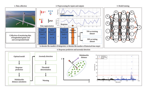
Anomaly detection involves tracking longitudinal displacements, essentially spotting atypical data points that notably diverge from expected patterns. Although the CMD could be directly derived from the measured girder end displacement, the proposed method has some advantages: (1) BNNs offer robust uncertainty quantification, which is crucial for understanding the level of confidence in predictions, especially in fluctuating conditions with inherent uncertainties due to environmental and load variations. (2) BNNs can predict displacement patterns over time, helping to identify subtle deviations that might not be apparent when examining CMD alone. (3) Incorporating predictive modeling within SHM increases robustness and provides probabilistic insights in operational conditions.

3. Algorithms for Displacement Prediction and Anomaly Detection

3.1. BNNs

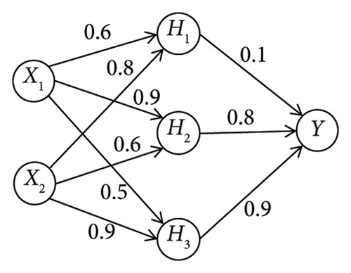
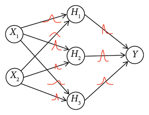
BNNs are a type of artificial neural network that incorporates Bayesian inference techniques into the modeling process. They are designed to provide uncertainty estimates along with predictions, making them useful in engineering scenarios where uncertainty quantification is important, such as in structural diagnosis, autonomous inspection, and response forecasting. BNNs are an extension of traditional backpropagate neural networks with some key differences: (1) Weight uncertainty: BNNs have distributions over weights, which capture uncertainty about the model’s parameters, as shown in Figure 2; (2) Bayesian inference: It allows BNNs to calculate not only point estimates (such as traditional neural networks) but also probabilistic estimates. BNNs will produce a distribution on possible outputs rather than a single output.

The BNNs are part of the probabilistic surrogate model denoted as P(y|x, w), in which x is the input, y is the output, w stands for the model parameters, and P signifies the probability distribution over possible output values. In the context of structural response regression, P(y|x, w) assumes the form of a Gaussian distribution, which corresponds to the utilization of squared loss. The weights can be learnt through MLE. In this context, when provided with a set of training examples denoted as $$, the MLE weights w^MLE are determined as follows:

$$ ()

This is accomplished using gradient descent or backpropagation under the assumption that the logarithm of the likelihood function $$ is differentiable with respect to the weights. To introduce regularization into the model, we can impose a prior distribution on the w. If w are assigned a Gaussian prior, it leads to L2 regularization. Conversely, if a Laplace prior is applied to w, it results in L1 regularization. In addition, we aim to find the MAP weights denoted as w^MAP

$$ ()

3.1.1. Variational Bayesian-Based Backpropagation

The training process in BNNs contains the Bayesian inference to assist the probabilistic modeling, instead of simply optimizing the neural network’s weights using backpropagation and gradient descent. A variational distribution, typically parameterized by learnable parameters, is introduced to approximate the true posterior distribution over weights. This distribution aims to match the true posterior as closely as possible. Variational Bayesian-based backpropagation is valuable in applications where understanding and quantifying confidence or uncertainty in predictions is essential.

Variational learning aims to determine the parameters θ of a weight distribution, denoted as q(w|θ), which minimizes the KL divergence from the true Bayesian posterior on weights, as defined in equation (3). This derived cost function is referred to by different names, including variational free energy [43] or the expected lower bound [44]. The cost function also could be simplified as equation (4), which can be referred to as the likelihood cost.

$$ ()

$$ ()

Equation (4) is the variational objective ($$). The first term is the KL divergence (D_KL) between the variational posterior and the prior, indicating the alignment of the weights with the prior distribution. The value of the second term hinges on the training dataset and quantifies the fitness between the model and data with the expected value under the variational distribution ($$). Optimizing objective equation (4) can be likened to a conventional regularization approach for practitioners, involving a trade-off between these two cost components.

3.1.2. Unbiased Monte Carlo Gradients

In equation (4), the existed expectation is challenging to compute directly. This challenge can be effectively tackled with Monte Carlo–based methods. It is well known that VAEs [45], derived from Bayesian estimation, introduced a clever reparameterization technique: For $$, directly sampling from $$ makes μ and σ nondifferentiable. To obtain their gradients, z is rewritten as z = σϵ + μ, where $$. This enables the sampling of the random variable ϵ from a standard Gaussian distribution while introducing μ and σ in a differentiable manner. For a random variable ϵ and probability density q(ϵ), as long as it adheres to the condition q(ϵ)dϵ = q(w|θ)dw, it becomes possible to derive a differentiable and unbiased estimate of the gradient with respect to the expectation:

$$ ()

Equation (5) is a generalization of the Gaussian reparameterization trick [46], originally designed for latent variable models, to the context of Bayesian learning. The Bayesian-based backpropagation method is specifically tailored for weight-based operations. Moreover, this approach is straightforward to implement and facilitates the interchangeability of different prior and posterior combinations. The approximation for the precise cost defined in equation (4) is as follows:

$$ ()

where w⁽ⁱ⁾ denotes the i th Monte Carlo sample drawn from the variational posterior q(w⁽ⁱ⁾|θ).

The utilization of a mixed-scale Gaussian prior, as illustrated in equation (7), can help define the form of P(w). In this setup, the prior distribution for each weight is a combination of two Gaussian distributions sharing the same mean but having different standard deviations. The subsequent step involves continued approximation of the objective function until a solution is attainable.

$$ ()

3.1.3. Minibatch Gradient Descent

The objective function in equation (4) and the approximation in equation (6) represent lower bounds for the model over the entire dataset. In neural network training, it is common to use minibatch gradient descent. Therefore, it is necessary to scale the complexity cost accordingly. Assuming the entire dataset is divided into m minibatches, the simplest approach is to take the average over each minibatch:

$$ ()

Simultaneously, equation (8) maintains conformity with the condition $$. Building upon this premise, equation (8) can also be rephrased as

$$ ()

As long as choosing π ∈ [0, 1]^m and ensuring that $$, the expression $$ serves as an unbiased estimation of $$. To elaborate further, if setting each π_i = 2^m−1/2^m − 1, it results in a particular weighting scheme that prioritizes aligning with the prior distribution during the initial stages of a single training epoch. As training progresses, it gradually shifts focus toward fitting the data. This strategic adjustment contributes to enhancements in overall model performance.

4. Data Acquisition From Bridge Health Monitoring System

4.1. The Bridge for Verification of the Method

Jiangyin Yangtze River Bridge stands as a suspension bridge in Jiangsu, China, with a substantial center span stretching 1385 m. Its opening to traffic in 1999 marked the first kilometer-level bridge in China. Functioning as a six-lane expressway, the bridge has a clearance height beneath the structure measuring 50 m.

Distinguished by nonsuspended north and south spans, the former extends 336.50 m, while the latter measures 309.34 m. The main cable has 169 parallel wire strands at the main span, maintaining a sag-to-span ratio of 1/10.5. Each strand comprises 127 galvanized steel wires with a 5.35-mm diameter. The adjacent suspending points are separated at 16 m, featuring two suspenders at each connection with the steel box girder. Suspender lengths surpassing 10 m consist of parallel wire strands, while those under 10 m employ stranded wire ropes.

A streamlined steel box girder carries the live loads, standing at 3.0 m in height. The top and bottom plate widths measure 29.50 and 22.94 m, respectively, culminating in a total width of 36.90 m. Tower heights differ, with the north tower reaching 183.85 m and the south tower at 186.85 m. The north and south anchorages adopt gravity-type concrete design and embedded concrete structure, respectively.

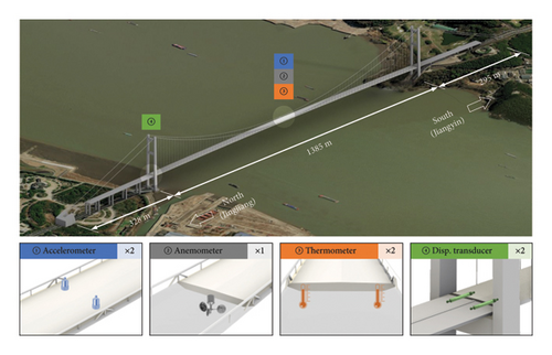
Subsequent to its 1999 inauguration for traffic, Jiangyin Yangtze River Bridge experienced the implementation of a SHM system to capture real-time data on environmental conditions and structural dynamic behavior. The array of sensors incorporated into this system encompasses anemometers, temperature gauges, strain sensors, GPS antennas, displacement gauges, and accelerometers. The selected sensors for this study are illustrated in Figure 3 for reference. Notably, the displacement gauges are strategically positioned longitudinally at the north and south towers of the steel box girder. These sensors employ a steel wire to record the displacements, operating at 20 Hz. Each cross section accommodates two temperature sensors on decks, totaling four sensors per section. Operating within a temperature range of −30°C to 85°C, these sensors continuously capture temperature data at 1 Hz.

4.2. Data Acquisition

To validate the proposed approach, an extensive set of continuous measurements spanning 12 days is gathered from the SHM of Jiangyin Bridge. The original data from the monitoring system undergo preprocessing to yield a dataset with a one-minute resolution for all parameters. This dataset configuration, comprising a significant volume of data, strikes a balance between providing ample datasets for training deep learning models and effectively characterizing various loads. A total of 20,160 data points are prepared to assess the efficacy of the developed method. The input variables encompass structural temperature, wind speed, and wind direction. Concurrently, the output variable targeted for prediction is the displacement of the bridge bearings.

4.2.1. Measured Loads

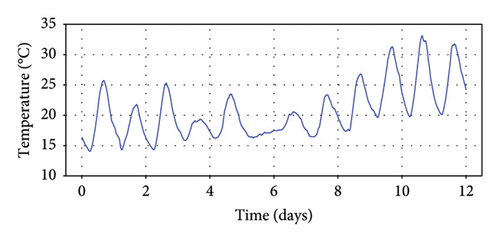
The fluctuation in temperature holds substantial significance in the design considerations of cable-supported bridges, necessitating careful and precise quantification. The input for the developed model is derived from the one-minute mean values of these temperature measurements. Figure 4 illustrates the 12-day dataset, revealing a discernible daily pattern influenced by the subtropical monsoon climate. Throughout this period, the recorded temperatures have exhibited a range from 14°C to 33°C, exemplifying the climatic variability in the area of the bridge.

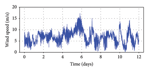
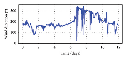
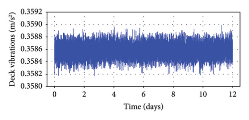
Due to their extended span and inherent flexibility, suspension bridges are particularly responsive to the impact of wind forces. A supersonic anemometer was positioned on the west side at the midspan. The signals captured by this instrument undergo processing at a one-minute interval. The wind speed and direction depicted in Figure 5 illustrate the distribution of measurements acquired over 12 days. Notably, the one-minute mean wind velocity can reach levels exceeding 18 m/s, indicative of moderately intense wind forces. For reference, the zero-degree reference is assigned to the north wind, while the east wind is denoted at 90°. Analysis of the wind direction reveals prevailing wind directions primarily in the northwest and west orientations. Figure 6 shows the measured vibrations of the main girder from the accelerometers, and it indicates the bridge is under normal operations in these days.

4.2.2. Longitudinal Displacements of Girder

Dynamic loads, such as strong winds and the passage of roadway vehicles, exert forces on the girder of cable-supported bridges, leading to deformations that can induce damage in various structural components, including expansion joints, bearings, and viscous damper. In response to these challenges, the concept of using CMD at the girder end as an index to estimate damage in such members has been proposed. This metric (CMD_j) is defined as the total accumulated displacement in a continuous period j, with $$ denoting the longitudinal displacements at the ith instances in the continuous period j.

$$ ()

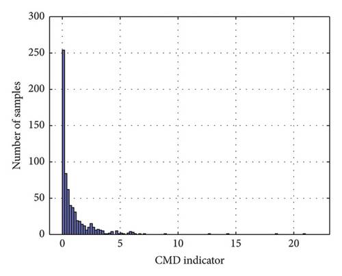
CMD emerges as a health condition indicator, reflecting the accumulated longitudinal girder movement within a specific time period. The distribution of the CMD indicator is visually represented in Figure 7.

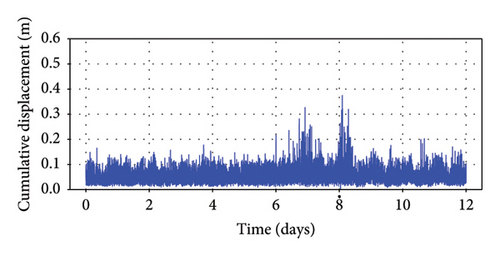
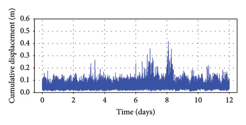
To obtain monitoring data for longitudinal displacement, measurements are taken from both the upstream and downstream locations of the northern extremity of the steel box girder. These extracted values are then utilized to calculate the CMDs at the girder ends for each minute. The results of these displacement calculations are depicted in Figure 8, where it is noteworthy that the amplitude of CMD within 1 minute may exceed 1 m.

5. Implementation and Discussion

The BNN model is trained utilizing the aforementioned loads and the longitudinal girder end displacement responses over a 12-day period, encompassing both the upstream and downstream sides of the structure. Denoising techniques are applied to mitigate noise interference. Historical load data are leveraged to enhance prediction accuracy. To ensure an appropriate denoised training and testing dataset, a split ratio of 7:3 is employed.

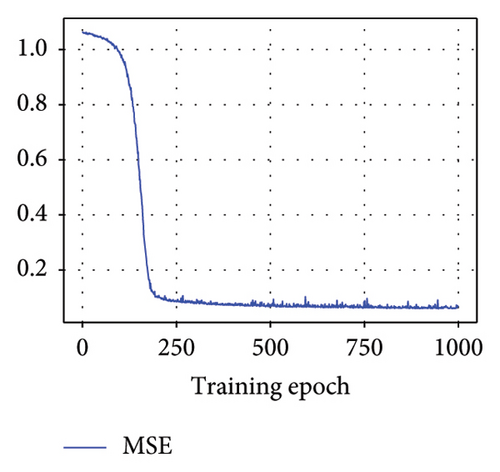
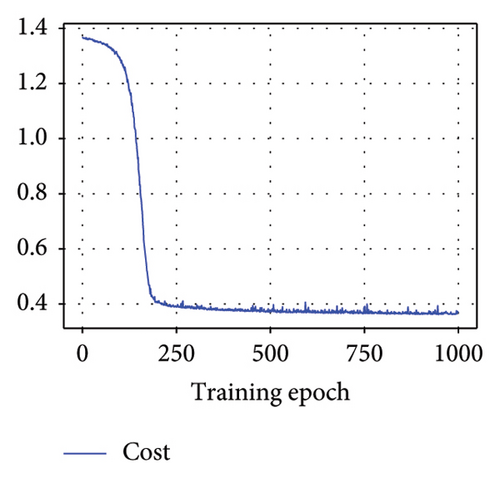
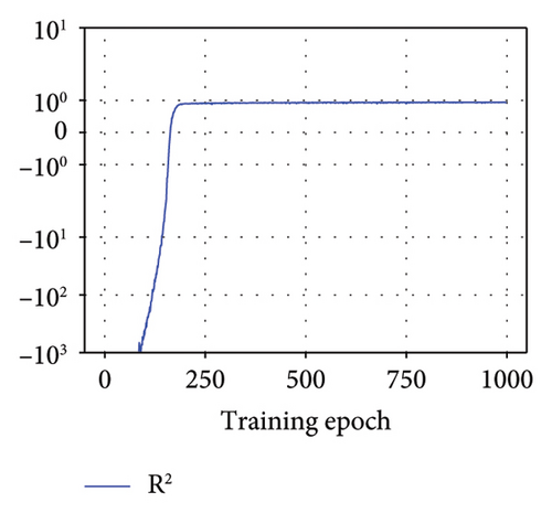
During the model training, MSE, total cost, and R² were employed to fine-tune the BNN model and identify optimal parameters. A desirable model exhibits a low MSE value, indicating minimal estimation error, and a high R² value, signifying a strong resemblance between predicted and actual responses. In addition, BNNs utilized the KL divergence between the variational posterior and the prior as a metric to quantify the model. This divergence measure offers insights into the alignment between these two probability distributions. A low total cost, as estimated by equation (6), serves as an indicator of the model’s strong performance in the realm of probability estimation.

5.1. Optimal Model Parameters

In order to guarantee the accuracy of the proposed BNN model in reconstructing longitudinal girder end displacement responses, we delve into the optimization of architectural parameters. Among these parameters, the number of hidden layers and neurons within each hidden layer is pivotal as they significantly impact the model’s architecture and performance. In Figure 9, several potential configurations for these parameters are investigated to assess their influence on model performance. The determination process is aided by employing R² and training time consumptions for comparison purposes.

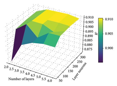
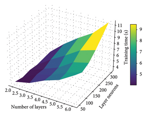
The evaluation of how changes in the number of hidden layers affect the model’s performance covers a range from 2 to 6 hidden layers. For the assessment of the number of neurons, we explored values ranging from 50 to 300. These comparative results of prediction accuracy and training time are depicted in Figures 9(a) and 9(b), respectively.

As the number of hidden layers increased, the estimation performance actually increased. Notably, the model with 3 hidden layers exhibited superior performance in displacement estimation while maintaining a good training efficiency. Beyond that, increasing the number of hidden layers led to seldom increase of prediction accuracy on the test dataset while increasing the training time. For layer neurons, it can be observed that an initial increase in the number of neurons improved displacement estimation performance. However, beyond a certain point, further increments in the number of neurons yielded limited gains in prediction accuracy. Consequently, the model with 150 neurons in each hidden layer emerged as the best-performing choice, offering a balance between performances and maintaining a relatively simple model architecture. Therefore, the optimal values for the number of hidden layers and the number of neurons are determined to be 3 and 150, respectively.

5.2. Model Tuning Procedure

Figure 10 displays the MSE, total cost, and R² metrics for the untrained test dataset with the optimal model. This study computes the average MSE, total cost, and R² across all steps within the epoch to represent the model performance. The MSE and total cost exhibit a notable reduction, converging to remarkably small values (MSE = 0.0686, cost = 0.389) and subsequently stabilizing. This trend indicates that the model achieves a high degree of prediction accuracy and demonstrates robust generalization capabilities. The model’s exceptional predictive performance is further substantiated by the consistently high R² value (0.9087), underscoring its proficiency in capturing underlying patterns in the data.

5.3. Prediction Results

Predicted outcomes accompanied by confidence estimates for untrained test data using the optimal BNN model on both the upstream and downstream sides are shown in Figure 11. These predictions were generated through the utilization of the optimal BNN model, applied to both the upstream and downstream sides. It is noteworthy that the R² for predictions on both sides exceeds 90%, underscoring the accuracy and precision of the model in capturing the underlying patterns in the data. This high R² value signifies a strong resemblance between the model’s predictions and the actual responses, reaffirming the model’s efficacy in delivering reliable and consistent results.

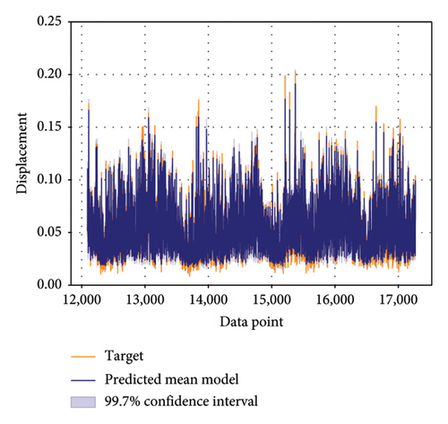
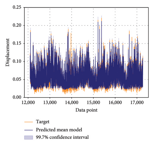
The confidence estimates that accompany the predicted outcomes provide valuable insights into the degree of certainty associated with each prediction. The elevated R² values observed on both the upstream and downstream sides underscore the model’s robustness in making probabilistic predictions. These outcomes highlight not just the model’s proficiency in generating precise point estimates but also its capability to furnish dependable indicators of uncertainty. This resilient probabilistic aspect of the model equips stakeholders with the tools to make informed decisions, all while considering the intrinsic uncertainties prevalent in real-world scenarios. It fosters a nuanced comprehension of the data and acknowledges the potential variations in the observed responses.

5.4. Anomaly Detection

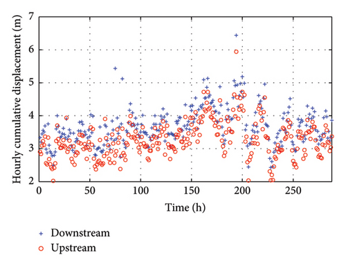
Anomaly detection typically involves comparing baseline data with target data samples. Establishing the baseline for anomaly detection entails processing the 12-day CMDs, measured in one-minute intervals, into hourly CMD values, as depicted in Figure 12. Analysis reveals that the hourly CMD ranges from 2 to 6.5 m.

Subsequently, the Mahalanobis distance is calculated following the procedures described previously, and its distribution is illustrated in Figure 13. Estimation of parameters via maximum likelihood for the GEV distribution yields values of 0.1568, 0.2544, and 1.3459 for the location, scale, and shape parameters, respectively. Since the shape parameter ξ_GEV is positive, the distribution follows a Type II or Fréchet extreme value distribution.

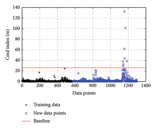
With the GEV distribution determined, a Monte Carlo simulation scheme is adopted to derive the 97% threshold as the reference for alarm. A total of 1 million samples are generated, resulting in a calculated threshold of 26.07. The sample size proves to be a large enough number to obtain the precise estimate, and the obtained value is taken as the baseline for warning of hourly CMD.

As shown in Figure 14, the training data represent the CMD index on both the upstream and downstream sides, while the new data are collected on bridge for 1 month. It is found that outliers appear in the newly collected datasets of the CMD index. As the index can reach as large as 130 m, there is a clear anomaly in the CMD, indicating damage in the components at the girder end. Inspection of the viscous dampers by engineers was carried out, which found malfunction due to leakage of high viscosity oil. The damper is illustrated in Figure 15. The malfunction caused deterioration in the damping of the device, and it was reflected in the proposed CMD index.

6. Conclusions

Note that the proposed two-stage framework and machine learning–based anomaly detection techniques leverage applicable concepts, such as BNNs and Mahalanobis distance, which can be adapted to various types of bridge structures. Future work will focus on validating this framework across a broader range of structures, including different bridge types and environmental conditions, to further substantiate its generalizability.

Disclosure

The interpretations and conclusions herein are solely the authors’ responsibility.

Conflicts of Interest

The authors declare no conflicts of interest.

Funding

This study was financially supported by the National Key Research and Development Program of China under grant contract No. 2023YFC3805902 and Southeast University’s Start-up Research Fund (RF1028623304).