1. Introduction

Bridge health monitoring system (BHMS) delivers an effective tool for evaluating the health status of bridges [1–3]. However, the monitoring data of BHMS are often affected by issues such as data missing and distortion due to the frequently occurring sensor failures [4] or noise interference [5]. These poor-quality data inevitably bring out an unreasonable estimation of bridge dynamic behaviors, even leading to improper decision-making in the following bridge usage and maintenance [6]. Hence, it is urgent to devise a precise method for recovering the bridge monitoring data.

The issues with the monitoring data missing can be classified into discrete and continuous data missing [7]. Among them, discrete data missing is characterized by data intermittently missing at the interval time points. For the problem of discrete data missing, the missing data can be extrapolated via utilizing the correlation between neighboring data points. For example, Lin et al. [8] employed a kriging-based sequence interpolation method to recover discrete data and obtained satisfactory results. Yang et al. [9] harnessed a priori knowledge of intrachannel sparsity and interchannel low-rank characteristics, employing L1-minimization and nuclear-norm minimization theories to recover randomly missing data. Zhang et al. [10] introduced an interpolation technique relying on the correlation between the changes of the measurement point data for recovering the discrete missing data. Chen et al. [11] introduced a probability density function estimation method based on the interpolation theory, utilizing the probability distribution of resultant data probability distribution to reconstruct the discrete missing strain monitoring data. For continuous data missing, it refers to the data missing in a continuous time period. Recovering continuous missing data is more challenging due to its typically greater missing length within a time period compared to discrete missing data. In this scenario, the above methods may be in trouble because the recovery fails to exploit the correlation between collected and missing data points [12].

To tackle the continuous data missing problem, those methods based on compressed sensing, machine learning, and deep learning have been developed [13]. Among them, the compressed sensing-based methods mainly employ the principle of signal sparsity for data recovery. Luo et al. [14] proposed an algorithm for selecting sparse sensors relying on data-driven to reconstruct aerodynamic characteristics of wind pressures on high-rise buildings from sparse measurement locations. Zou et al. [15] utilized a compressive sensing method based on the random demodulator to recover the lost data during the signal transmission of structural health monitoring systems. Bao et al. [16] developed a combined method integrating data mapping and compressed sampling, achieving the recovery of measured acceleration data. Second, machine learning–based methods establish the link between input features and target variables, thereby enabling the prediction of missing data through the mapping relationship [17, 18]. For example, Zhang et al. [19] presented a Bayesian dynamic regression approach for restoring missing monitoring data, enhancing computational efficiency and recovery accuracy. Wan and Ni [20] introduced a Bayesian multi-\task learning method for recovering the temperature and acceleration data, achieving the improvement of recovery accuracy. Huang, Li, and Han [21] proposed a method utilizing correlation analysis combined with machine learning to recover the missing wind pressure data. Although the above methods have made some progress in recovering continuous missing data, these studies mainly focus on scenarios with low missing rates, as shown in Table 1. The recovery capability for scenarios with high missing rates has not been fully explored and deserves several further investigations [22, 23].

As artificial intelligence progresses constantly, deep learning has exhibited a powerful potential in addressing the continuous missing data. Deep learning models are adept at learning and extracting deep features from the data through the nonlinear mapping capabilities of multilayer neural networks [24], thereby facilitating the effective recovery of continuous missing data [25]. Ju et al. [26] introduced a bidirectional forecasting approach utilizing a gated recurrent unit (GRU) model to recover the data of beam-end displacements and pylon tower tilts. Liu et al. [27] presented a method grounded in long short–term memory (LSTM) neural networks to recover the bridge structure temperature data. Liu et al. [28] adopted a wavelet-based residual neural network to recover the missing seismic data. Jeong et al. [29] presented a bidirectional recurrent neural network (RNN) designed to utilize the temporal correlation among sensor data for recovering the missing acceleration data. Lei, Sun, and Xia [30] introduced a deep convolutional generative adversarial network (GAN) with an encoder–decoder structure to recover the missing acceleration data. However, a single deep learning model exhibits insufficient generalization capabilities in handling data with diverse features [31]. To effectively mine more features in the data, the concept of model ensemble design has gradually emerged as a new development trend in the field of signal recovery. For instance, Fan, He, and Li [32] proposed the GAN, combining the self-attention mechanism to capture intrinsic linkages in the data, thereby facilitating the recovery of missing data. Wang et al. [25] developed a method integrating LSTM and U-net to reconstruct beam-end displacement data. Chen et al. [33] proposed a hybrid model combining autoregressive (AR) models, BiGRU, and convolutional neural networks (CNNs) to recover the strain data. However, integrating multiple computationally complex submodels within a composite model may lead to multicollinearity issues due to the high correlation among features extracted by the submodels, thereby reducing the recovery accuracy [34, 35]. More importantly, these deep learning models cannot capture the nonstationarity embedded in the data, resulting in limited recovery accuracy [23].

To mitigate the complexity of nonstationary signals, methods such as empirical mode decomposition (EMD) [36] and variational mode decomposition (VMD) [37] have been utilized in the signal recovery. For example, Li et al. [38] utilized the EMD-assisted LSTM model to reconstruct the bridge acceleration data. Liu et al. [39] utilized EMD-assisted BiGRU to recover the missing acceleration data with significant improvement in terms of recovery accuracy. He, Guan, and Liu [40] introduced a method integrating intermittent criteria-based EMD with finite element modeling to achieve the dynamic response reconstruction. Zhu et al. [41] proposed an optimized bidirectional LSTM method based on VMD for the strain data recovery. However, signal decomposition techniques such as EMD often suffer from endpoint effects and mode aliasing problems [23]. Although VMD can address these problems to some extent, it is difficult to accurately assess the frequency characteristics near the signal endpoints. Meanwhile, the key parameters of VMD such as the decomposition mode number and the balance factor are determined based on the experience of users and usually lack sufficient robustness [42]. Fortunately, a signal decomposition technique called successive VMD (SVMD) can effectively overcome these issues. This technique not only has the advantages of improving the endpoint effect and mode aliasing of traditional decomposition methods but also dispenses with any prior knowledge of important parameter settings. This technique can reduce the sensitivity on the initialization of center frequency and computational complexity [43]. Therefore, the application of SVMD in the field of signal recovery may be promising.

Building upon the insights from the above studies, this paper proposes an innovative SVMD-assisted deep learning composite model for the recovery of continuous missing signals. In this method, SVMD with high reliability and strong robustness is employed to extract the data-embedded time-frequency characteristics. Then, the combination of temporal convolutional networks (TCNs), multihead attention (MHA), and bidirectional GRUs (BiGRUs), i.e., TCN–MHA–BiGRU, is designed to comprehensively capture the data-contained time-series characteristics. A case study using data from BHMS demonstrates the efficacy of the proposed method.

The paper is structured as follows. The theory employed in this study is offered in detail in Section 2. The proposed signal recovery method is described in Section 3. The recovery effect of the method in the case of long-term signal missing is demonstrated in Section 4. The performance of the proposed method under varying data missing rates and different numbers of complete data is analyzed in Section 5. The applicability of the method to short-term datasets is analyzed in Section 6. Section 7 presents the conclusion of the study.

2. Theoretical Background

3. Proposed Method

The proposed method primarily encompasses three aspects, i.e., SVMD-based signal decomposition, TCN–MHA–BiGRU–based subseries prediction, and linear integration. The specific illustration regarding each involved aspect will be expounded in the following sections.

3.1. Signal Recovery Process

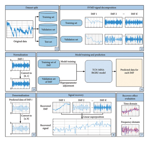
Figure 1 presents the entire procedure of the proposed method, with the details elaborated as follows.

3.1.1. Dataset Split

According to the model complexity and dataset size, the dataset is reasonably split to assure the effective training of the model [49], with the training set X₁ = {x₁, x₂, …, x_c−1, x_c}, the validation set X₂ = {x_c+1, x_c+2, …, x_c+m−1, x_c+m}, and the test set X₃ = {x_c+m+1, x_c+m+2, …, x_c+m+n−1, x_c+m+n} having lengths of c, m, and n, respectively. They are applied sequentially to model training, hyperparameter tuning, and recovery performance evaluation.

3.1.2. SVMD-Based Signal Decomposition

The training and validation set data sequences are decomposed to obtain K IMFs using SVMD, i.e., U_i = {u_i,1, u_i,2, …, u_i,c−1, u_i,c}, $$, where i = 1, 2, …, K, U_i is the i-th IMF of the training set, $$ is the i-th IMF of the validation set, and u_i,c is the c-th data of the i-th IMF. The details of the SVMD can be found in Section 2.1.

3.1.3. Data Normalization

The data of each IMF is min–max normalized, i.e.,

$$ ()

where $$ is the result of the normalization of the c-th data in the i-th IMF. The normalized data range is [0, 1] for eliminating the negative impact caused by the order of magnitude difference in data on the subsequent model training and prediction.

3.1.4. TCN–MHA–BiGRU–Based Model Training and Prediction

For each set of IMFs, the corresponding TCN–MHA–BiGRU model is established, with IMFs from the training set and the validation set fed into the model during training. On this basis, each trained model is employed to predict the corresponding missing IMF, i.e., {u_i,c+m+1, u_i,c+m+2, …, u_i,c+m+n}. More information on the developed TCN–MHA–BiGRU model can be found in Section 3.2.

3.1.5. Denormalization

To convert the predicted values into the same range and scale as the original data, the predicted IMFs are denormalized to obtain each recovered IMF $$, where $$ indicates the j-th data of the i-th recovery IMF.

3.1.6. Signal Recovery

By linearly superposing all the predicted IMFs, the final recovery signal $$ is generated, with the calculation formula for $$ as follows:

$$ ()

where $$ denotes the j-th recovery data.

3.1.7. Recovery Effect Evaluation

The evaluation of recovery results through comprehensive time-frequency analysis, with the evaluation metrics, is detailed in Section 3.3.

3.2. TCN–MHA–BiGRU

The signal recovery model utilized in this article integrates TCN, MHA, and BiGRU. Among them, TCN can be well-suited for capturing linear and nonlinear features due to the convolutional operation [50]. MHA learns the correlation among different positions of the input sequence and the importance of different features to achieve feature enhancement [46]. The bidirectional cyclic structure of BiGRU provides the ability to model global dependencies in the time series [51]. Therefore, the combination of TCN and BiGRU in a functional complementary way is beneficial to adequately describe the temporal features embedded in the monitoring data. By incorporating MHA into the TCN–BiGRU network, the effectiveness of utilizing data information can be further enhanced. This combination is designed to fully exploit the strengths of each submodel to enhance the recovery accuracy. Within this composite model, the task allocation for different models is as follows: (1) Designs such as dilated causal convolution and residual connection in TCN are utilized to precisely capture the linear and nonlinear characteristics of the signal data sequence. (2) To enhance the ability of the network to capture data dependencies and focus on important features in the presence of abundant outlier data, MHA is employed to assign corresponding attention weights to outlier and steady data. (3) The global information of the signal is extracted bidirectionally through BiGRU to enhance the model’s ability to understand the overall trend of the signal. This division of labor design effectively prevents multicollinearity issues caused by the high similarity of features extracted among the submodels. Figure 2 shows the structure of the TCN–MHA–BiGRU composite model. Specific descriptions of each submodel have been given in Section 2. The detailed procedure for this composite model is outlined as follows:

•  

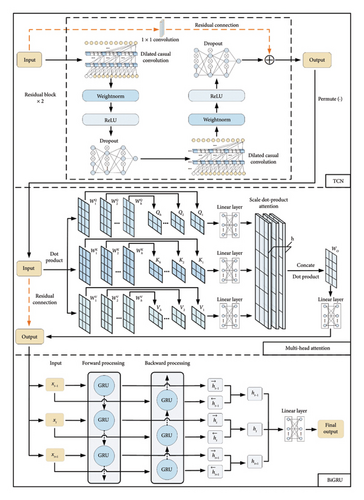
  Step 1: TCN performs convolutional operations on the input time series and utilizes residual connections to propagate feature information across layers, capturing linear and nonlinear data characteristics. TCN comprises two residual blocks with output dimensions of 32 and 64, respectively.

•  

  Step 2: Utilizing the permute (·) function, the output of the TCN model is dimensionally adjusted to facilitate its feeding into MHA.

•  

  Step 3: The data are processed after TCN feature mapping using MHA, calculating the attentional weights of the outlier data points and the steady data points. The attention heads are configured to a total of 8.

•  

  Step 4: Employing residual connections again to elementwise, the input and output of MHA are added, enabling the cross-layer propagation of features extracted by TCN and preserving detailed information. This also aids in mitigating the occurrence of gradient vanishing or explosion, thereby allowing for the training of deeper networks.

•  

  Step 5: Utilizing the bidirectional gating mechanism of BiGRU, the multidimensional time-dependent features fused after processing through TCN and MHA are further refined to extract global time series characteristics. BiGRU fuses the bidirectionally extracted data features and performs the missing data prediction, with both forward and backward GRU units having an internal hidden state dimensionality of 64.

•  

  Step 6: Finally, the output of BiGRU is mapped to the target dimension by a linear layer, with the output at the last time step serving as the ultimate prediction result.

4. Experimental Verification

4.1. Data Sources and Experimental Background

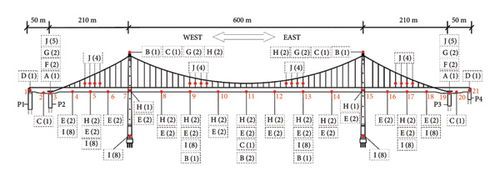
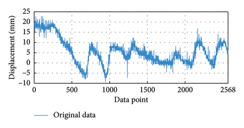
The experimental data are derived from the BHMS installed on a bridge in Chongqing, China. The bridge is a self-anchored large-span suspension bridge with steel box girders for the center and side spans, and a reinforced concrete structure for the main tower. Sensors and other monitoring devices are installed at key structural points including the pier tops, outer sides along the bridge deck, bridge towers, and suspension cables for real-time monitoring of bridge status, as displayed in Figure 3. This experiment takes the horizontal displacement data of bridge pier P2 on the west side at Measurement point 3, sampled at 1/300 Hz. A total of 2568 data were collected after 0:00 on December 8, 2023. The data are shown in Figure 4.

4.3. Signal Decomposition and Data Normalization

To decrease the signal complexity and nonstationarity as well as to extract the different frequency components, the data corresponding to the training and validation sets are decomposed using SVMD. The SVMD parameters are configured as follows: the sampling frequency is 1/300 Hz, the maximum (Max.) balancing parameter value (α_max) takes 300, and the minimum (Min.) balancing parameter value (α_min) takes 10 [42, 43]. A total of four IMFs are obtained from the decomposition, as shown in Figure 5. To demonstrate the signal decomposition performance of SVMD, the overlap rate of bandwidths between neighboring IMFs is computed, with a lower value indicating a lighter degree of modal aliasing [52]. The bandwidth of each IMF refers to the mean ± standard deviation (Std.) of the corresponding IF, and the bandwidth overlap rate refers to the percentage of the overlapping bandwidth between two adjacent IMFs relative to their total bandwidth. In this experiment, three signal decomposition techniques, including EMD, VMD and time-varying filter-based EMD (TVFEMD), are selected to participate in the comparison. To avoid an excessive number of decomposition modes leading to the accumulation of prediction errors in subsequent models and improve operational efficiency [58, 59], the Max. number of decomposition levels is limited to 4 for all techniques [23].

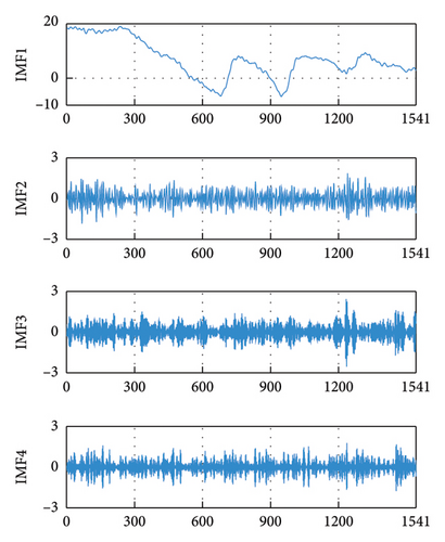
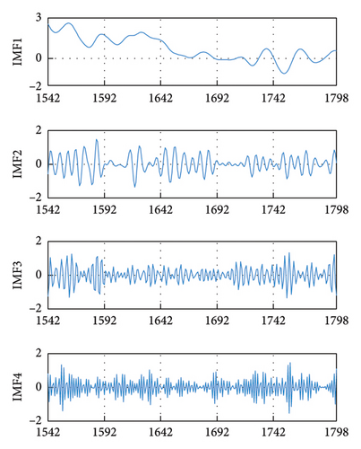
From Table 2, it is observed that the bandwidth overlap rate among SVMD-based IMFs is lower than those of other signal decomposition techniques, which indicates a superior decomposition performance of SVMD. In addition, it can be seen that the two improved signal decomposition methods, SVMD and TVFEMD, have lower average (avg.) values of bandwidth overlap ratio with respect to the traditional signal decomposition techniques, VMD and EMD, respectively. After the decomposition is complete, each IMF is normalized to eliminate the impact of data magnitude differences on model training.

Table 2. Bandwidth overlap rates for four signal decomposition techniques.

Technique	IMF–IMF2	IMF2–IMF3	IMF3–IMF4	Average overlap rate (%)
SVMD	0	0	20.32%	6.77
VMD	0	0	29.76%	9.92
EMD	4.02%	36.92%	32.67%	24.54
TVFEMD	30.62%	38.61%	0	23.08

4.4. Model Training

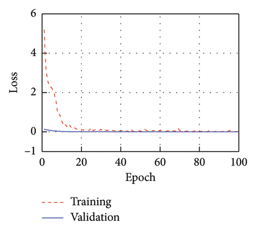
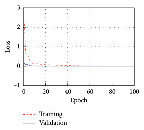
For these decomposed IMFs, four different TCN–MHA–BiGRU models are, respectively, established. In these models, AdamW and MSE are used as the optimizer and loss function, respectively. The model hyperparameters are configured as follows: learning rate of 0.001, training epoch of 100, and batch size of 64. To prevent overfitting, the weight decay coefficient and dropout take 0.001 and 0.1, respectively [60].

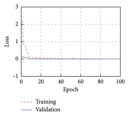
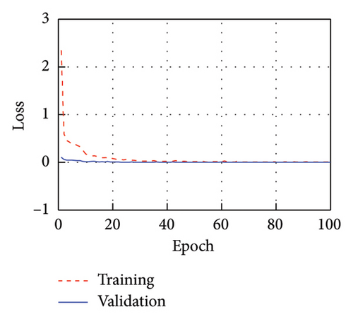
Figure 6 displays the training process of models corresponding to each IMF, with both the training and validation loss (Val.) curves demonstrating rapid convergence. Upon reaching 100 training epochs, the MSE for each model on the training set is 0.0252, 0.0047, 0.0138, and 0.0094, while the MSE on the validation set is 0.0010, 0.0007, 0.0038, and 0.0008, respectively. Throughout the training process, the MSE on the validation set remains generally lower than the training set, indicating the absence of overfitting.

4.5. Signal Recovery

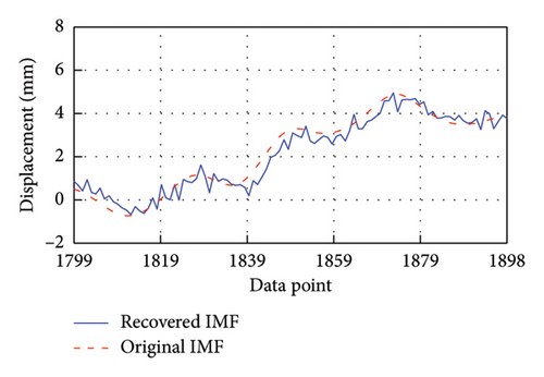
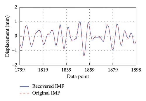
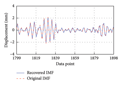
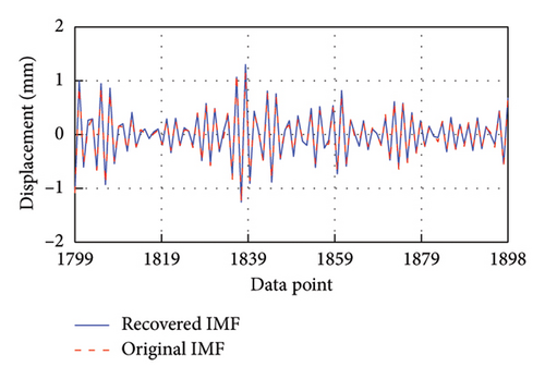
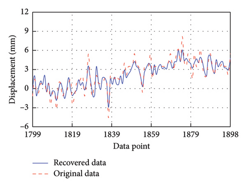
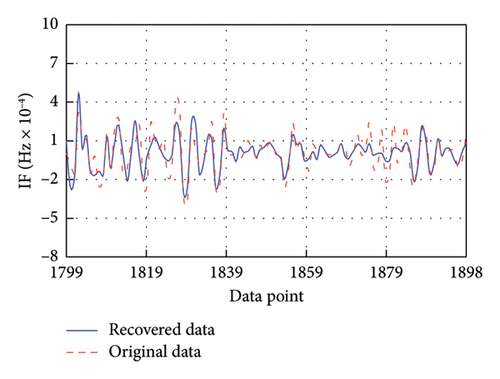
After training, these models are employed to predict the corresponding missing IMF data. To facilitate clear observation, Figure 7 takes the first 100 recovered data for each IMF as an example to display the recovery results. It is evident that the four recovered IMFs generally align with the original IMFs. Subsequently, all recovered IMFs are linearly superimposed to obtain the final recovery data. On this basis, the HT is utilized to acquire the IF of the recovery result. As shown in Figure 8, the recovered data exhibit excellent time-frequency alignment with the original data.

4.6. Evaluation and Comparison

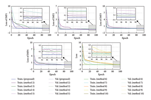
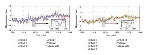
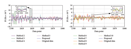
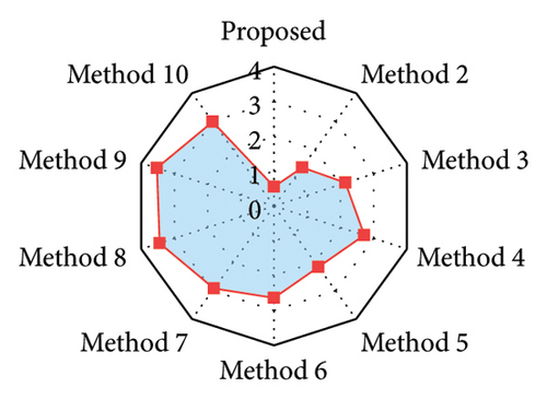
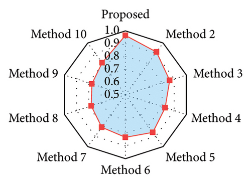
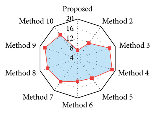
To verify the superiority of the proposed method, four methods based on signal decomposition and five methods not based on signal decomposition are selected for the comparison of time-frequency domain recovery results. The corresponding methods are listed in Table 3. Among them, three advanced data recovery methods (i.e., Method 4, Method 5, and Method 10) are derived from the literature [13, 27, 38], respectively. To ensure fairness, the number of training epochs for each method is 100. Figure 9 displays the training process for each method, and Table 4 gives the Min. training loss (Train.) and Val. as well as the corresponding training time. It can be seen that these methods based on signal decomposition techniques have a longer training time due to the repeated prediction operation for each subseries. The proposed method achieves the fastest convergence for each IMF and has the lowest loss on both the training and validation sets among all the methods based on signal decomposition techniques. In addition, the comparison among all methods without signal decomposition techniques indicates that although the developed TCN–MHA–BiGRU model has a higher model complexity, it achieves the lower Train. and Val..

Table 3. Illustration of different recovery methods.

Method	Decomposition techniques	Model
Proposed method	SVMD	TCN–MHA–BiGRU
Method 2	VMD	TCN–MHA–BiGRU
Method 3	EMD	TCN–MHA–BiGRU
Method 4	EMD	LSTM
Method 5	TVFEMD	ED-LSTM
Method 6	/	TCN–MHA–BiGRU
Method 7	/	TCN–BiGRU
Method 8	/	TCN
Method 9	/	BiGRU
Method 10	/	LSTM

Table 4. Minimum loss during training and training time for each method.

Method	Train./val.	Minimize training loss and validation loss					Training time (s)
		IMF1	IMF2	IMF3	IMF4	Undecomposed data
Proposed	Train.	0.0144	0.0047	0.0097	0.0069	/	418.92
	Val.	0.0007	0.0005	0.0009	0.0008	/
Method 2	Train.	0.0619	0.0637	0.1392	0.1422	/	419.72
	Val.	0.0075	0.0050	0.0125	0.0135	/
Method 3	Train.	0.0721	0.2548	0.0600	0.0974	/	426.76
	Val.	0.0110	0.0332	0.0071	0.0119	/
Method 4	Train.	0.2367	0.2817	0.1285	0.1794	/	348.05
	Val.	0.0251	0.0367	0.0186	0.0143	/
Method 5	Train.	0.0958	0.1185	0.2734	0.0547	/	397.51
	Val.	0.0258	0.0158	0.0360	0.0054	/
Method 6	Train.	/	/	/	/	0.0661	119.29
	Val.	/	/	/	/	0.0079
Method 7	Train.	/	/	/	/	0.0779	104.19
	Val.	/	/	/	/	0.0134
Method 8	Train.	/	/	/	/	0.1412	87.16
	Val.	/	/	/	/	0.0160
Method 9	Train.	/	/	/	/	0.1537	94.22
	Val.	/	/	/	/	0.0183
Method 10	Train.	/	/	/	/	0.1116	99.25
	Val.	/	/	/	/	0.0155

The recovery results are exhibited in Figure 10. The evaluation metric values for each method are presented in Table 5. The rate of change in evaluation metrics for the proposed method relative to other methods is detailed in Table 6 and further visualized in Figure 11. The following observations can be found:

• 1.

  Among these methods based on signal decomposition techniques, the SVMD-based method demonstrates the best time-frequency recovery performance. From the time-domain perspective, compared to VMD- and EMD-based methods, this SVMD-based method realizes the corresponding reduction of RMSE by 36.62% and 49.41% and MSE by 59.82% and 74.40%, while increasing R² by 5.41% and 10.55%, respectively. From the frequency domain aspect, the drop in RMSEIF is 37.09% and 58.15%, respectively. This indicates that decomposition results from SVMD may be better suited for subsequent recovery. This technique is capable of adaptively decomposing the signal into multiple stable subsequences without prior knowledge of crucial parameters and effectively extracts the time-frequency characteristics of the signal.

• 2.

  Among those methods without employing signal decomposition techniques, the TCN–MHA–BiGRU composite model surpasses all the other single models regarding recovery effectiveness in the time-frequency domains. For instance, the RMSE, MSE, and RMSEIF are reduced by 12.60%, 23.61%, and 20.90%, respectively, and the R² is enhanced by 6.22% relative to TCN. This may result from the proposed model integrating the advantages of individual models, thereby enhancing the capability to extract data features. In addition, several experiments (i.e., comparisons of Methods 6, 7, 8, and 9) show that the combination of BiGRU and TCN (i.e., TCN–BiGRU) enhances the recovery accuracy, and the fusion of MHA with BiGRU–TCN delivering additional improvement. For example, TCN–BiGRU reduces RMSE by 7.97% and 8.93% compared to TCN and BiGRU, while RMSEIF decreases by 6.62% and 12.65%, respectively. Furthermore, combining MHA with TCN–BiGRU, respectively, reduces RMSE and RMSEIF by 5.04% and 15.30% relative to TCN–BiGRU. This demonstrates that TCN–MHA–BiGRU can effectively avoid the multicollinearity problem, and thus this combined architecture is reasonable and reliable.

• 3.

  Among all comparison methods, the proposed method of the SVMD-based TCN–MHA–BiGRU model exhibits the best performance in time-frequency aspects. In the time domain, the proposed method exhibits the minimal RMSE and MSE, along with the highest R². In the frequency domain, it still maintains superior recovery capabilities, with an RMSEIF as low as 7.3627 × 10⁻⁵. For example, the proposed method reduces RMSE by 55.01%, 49.49%, and 57.11%, with RMSEIF reductions of 60.51%, 46.98%, and 53.58% compared to Methods 4, 5, and 10, respectively. It should be noted that Method 5 exhibits better recovery accuracy in both the time and frequency domains compared to Method 4. Although the recovery accuracy of Method 4 is improved in the time domain relative to Method 10, its frequency domain recovery accuracy is lower. Therefore, it is beneficial to select suitable signal decomposition techniques and models to improve the recovery level in the time-frequency domain. In addition, based on the comparison of Method 4 and Method 5, it can be found that the TVFEMD and ED-LSTM–based methods provide better recovery results relative to the EMD- and LSTM-based methods. This indicates the importance of optimization and improvement on traditional signal decomposition techniques and models to enhance the recovery accuracy.

Table 5. Evaluation metrics of different methods.

Method	RMSE	MSE	R2	RMSEIF (× 10−5)
Proposed	0.7421	0.5507	0.9650	7.3627
Method 2	1.1708	1.3707	0.9128	11.7034
Method 3	1.4668	2.1514	0.8632	17.5909
Method 4	1.6496	2.7211	0.8269	18.6421
Method 5	1.4692	2.1584	0.8627	13.8858
Method 6	1.6238	2.6367	0.8323	13.2477
Method 7	1.7099	2.9238	0.8140	15.6398
Method 8	1.8579	3.4518	0.7805	16.7487
Method 9	1.8775	3.5249	0.7758	17.9047
Method 10	1.7304	2.9943	0.8096	15.8617

Table 6. Comparison of evaluation metrics between the proposed method and other methods.

Method	RMSE (%)	MSE (%)	R2 (%)	RMSEIF (%)
Method 2	−36.62	−59.82	+5.41	−37.09
Method 3	−49.41	−74.40	+10.55	−58.15
Method 4	−55.01	−79.76	+14.31	−60.51
Method 5	−49.49	−74.49	+10.60	−46.98
Method 6	−54.30	−79.11	+13.75	−44.42
Method 7	−56.60	−81.16	+15.65	−52.92
Method 8	−60.06	−84.05	+19.12	−56.04
Method 9	−60.47	−84.38	+19.61	−58.88
Method 10	−57.11	−81.61	+16.10	−53.58

5. Robustness and Sensitivity Analysis

In order to verify the robustness and sensitivity of the proposed method to changes in the missing rate as well as the number of complete data, this section discusses these two scenarios in detail in Sections 5.1 and 5.2, respectively.

5.1. Missing Rate

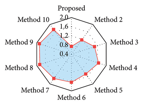
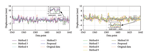
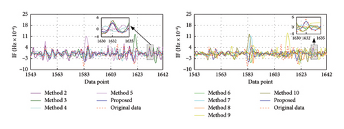
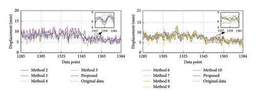
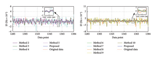
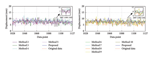
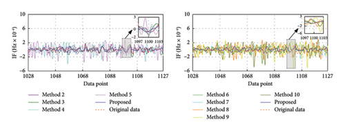
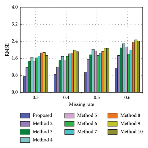
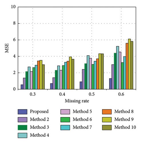
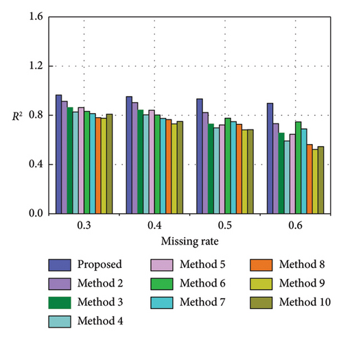
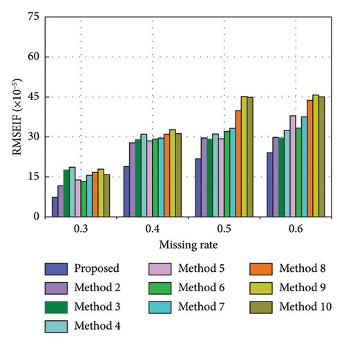
To evaluate the efficacy of the proposed method under various missing rates, this section investigates its recovery effects at missing rates of 40%, 50%, and 60%, respectively. The corresponding missing data series are {x₁₅₄₃, x₁₅₄₄, …, x₂₅₆₈}, {x₁₂₈₅, x₁₂₈₆, …, x₂₅₆₈}, and {x₁₀₂₈, x₁₀₂₉, …, x₂₅₆₈}, respectively. Figures 12, 13, and 14 exhibit the recovery results in the time-frequency domain for all involved methods under the three missing rates. The evaluation metrics and training time for various methods under different missing rates are presented in Tables 7, 8, and 9 and further visualized in Figure 15. The rate of change in the evaluation metrics for the proposed method in comparison to other methods under varying missing data rates is presented in Tables 10, 11, and 12. According to the recovery results, it can be observed that recovery errors of all methods gradually increase as the missing rate rises based on time-frequency analyses. This is likely attributed to the fact that as the data missing rate rises, the available data features for extraction decrease, rendering the recovery process relatively more challenging. It is worth noting that the developed TCN–MHA–BiGRU outperforms other models in recovery performance across different missing rates, although it requires a longer training time. In addition, the proposed method consistently maintains the highest level of recovery accuracy, which can be ascribed to the superiorities of SVMD in extracting time-frequency characteristics and TCN–MHA–BiGRU in mining time-series characteristics.

Table 7. Evaluation metrics and training time (40% missing rate).

Method	RMSE	MSE	R2	RMSEIF (× 10−5)	Training time (s)
Proposed	0.8390	0.7040	0.9518	18.9305	362.86
Method 2	1.1902	1.4166	0.9030	27.8048	367.51
Method 3	1.5182	2.3050	0.8422	29.0691	369.42
Method 4	1.6900	2.8559	0.8045	31.0401	330.65
Method 5	1.5218	2.3158	0.8414	28.5413	345.86
Method 6	1.6996	2.8886	0.8022	29.1582	104.86
Method 7	1.8138	3.2897	0.7748	29.5580	95.64
Method 8	1.8493	3.4200	0.7658	31.0237	80.94
Method 9	1.9851	3.9407	0.7302	32.7424	86.69
Method 10	1.9116	3.6542	0.7498	31.2008	91.45

Table 8. Evaluation metrics and training time (50% missing rate).

Method	RMSE	MSE	R2	RMSEIF (× 10−5)	Training time (s)
Proposed	0.9581	0.9179	0.9324	21.7983	340.57
Method 2	1.5568	2.4235	0.8214	29.6044	344.96
Method 3	1.7672	3.1229	0.7290	29.1760	347.74
Method 4	2.0240	4.0964	0.6982	31.1004	314.06
Method 5	1.9445	3.7812	0.7214	29.2896	326.98
Method 6	1.7397	3.0264	0.7770	32.0631	95.62
Method 7	1.8455	3.4060	0.7491	33.2078	86.55
Method 8	1.9241	3.7023	0.7272	39.8456	75.64
Method 9	2.0796	4.3249	0.6814	45.1324	78.36
Method 10	2.0758	4.3088	0.6825	44.8741	82.62

Table 9. Evaluation metrics and training time (60% missing rate).

Method	RMSE	MSE	R2	RMSEIF (× 10−5)	Training time (s)
Proposed	1.1459	1.3131	0.8973	24.0427	315.85
Method 2	1.7340	3.0067	0.7324	29.7984	318.79
Method 3	2.0966	4.3958	0.6562	29.6306	319.68
Method 4	2.2866	5.2284	0.5911	32.5189	286.43
Method 5	2.1300	4.5369	0.6452	37.9128	307.15
Method 6	1.8030	3.2509	0.7457	33.3306	86.45
Method 7	1.9930	3.9720	0.6893	37.5648	77.63
Method 8	2.3658	5.5968	0.5623	43.6887	67.63
Method 9	2.4717	6.1094	0.5222	45.7018	70.78
Method 10	2.4121	5.8183	0.5449	45.0361	74.35

Table 10. Comparison of evaluation metrics between the proposed method and other compared methods (40% missing rate).

Method	RMSE (%)	MSE (%)	R2 (%)	RMSEIF (%)
Method 2	−29.51	−50.30	+5.13	−31.92
Method 3	−44.74	−69.46	+11.52	−34.88
Method 4	−50.36	−75.35	+25.12	−39.01
Method 5	−44.87	−69.60	+11.60	−33.67
Method 6	−50.64	−75.63	+15.72	−35.08
Method 7	−53.74	−78.60	+18.60	−35.96
Method 8	−54.63	−79.42	+19.54	−38.98
Method 9	−57.74	−82.14	+23.28	−42.18
Method 10	−56.11	−80.74	+21.22	−39.33

Table 11. Comparison of evaluation metrics between the proposed method and other compared methods (50% missing rate).

Method	RMSE (%)	MSE (%)	R2 (%)	RMSEIF (%)
Method 2	−38.46	−62.13	+11.91	−26.37
Method 3	−45.78	−70.61	+21.82	−25.29
Method 4	−52.66	−77.59	+25.12	−29.91
Method 5	−50.73	−75.72	+22.63	−25.58
Method 6	−44.93	−69.67	+16.67	−32.01
Method 7	−48.09	−73.05	+19.66	−34.36
Method 8	−50.21	−75.21	+22.01	−45.29
Method 9	−53.93	−78.78	+26.92	−51.70
Method 10	−53.84	−78.70	+26.80	−51.42

Table 12. Comparison of evaluation metrics between the proposed method and other compared methods (60% missing rate).

Method	RMSE (%)	MSE (%)	R2 (%)	RMSEIF (%)
Method 2	−33.92	−56.33	+18.38	−19.32
Method 3	−45.35	−70.13	+26.87	−18.86
Method 4	−49.87	−74.89	+34.13	−26.07
Method 5	−46.20	−71.06	+28.10	−36.58
Method 6	−36.45	−59.61	+16.90	−27.87
Method 7	−42.50	−66.94	+23.18	−36.00
Method 8	−51.56	−76.54	+37.33	−44.97
Method 9	−53.64	−78.51	+41.81	−47.39
Method 10	−52.49	−77.43	+39.27	−46.62

5.2. The Number of Complete Data

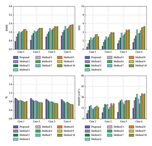
To assess the recovery effectiveness of the proposed method under different numbers of complete data, this section assumes that the number of complete data points is reduced sequentially by 10% of the original data based on Section 4, as listed in Table 13. It needs to be noted that Case 1 is the experiment discussed in Section 4. The evaluation metrics and training times of the involved methods in each case are shown in Tables 14, 15, and 16, respectively. Figure 16 further visualizes these metrics. The corresponding change rate of each method with respect to the proposed method is given in Tables 17, 18, and 19.

Table 13. Different cases of complete data quantities.

Case	The number of complete data	The number of missing data	Complete data	Missing data
Case 1	1798	770	{x1, x2, …, x1798}	{x1799, x1800, …, x2568}
Case 2	1540	770	{x259, x260, …, x1798}	{x1799, x1800, …, x2568}
Case 3	1284	770	{x515, x516, …, x1798}	{x1799, x1800, …, x2568}
Case 4	1028	770	{x771, x772, …, x1798}	{x1799, x1800, …, x2568}

Table 14. Evaluation metrics and training time (Case 2).

Method	RMSE	MSE	R2	RMSEIF (× 10−5)	Training time (s)
Proposed	0.8646	0.7475	0.9525	8.6119	365.91
Method 2	1.3046	1.7020	0.8918	15.3754	369.93
Method 3	1.5024	2.2571	0.8564	20.4870	371.39
Method 4	1.7237	2.9711	0.8110	19.0236	332.15
Method 5	1.5774	2.4882	0.8418	20.1745	342.33
Method 6	1.6890	2.8528	0.8186	13.4253	107.37
Method 7	1.8541	3.4375	0.7814	15.9825	98.72
Method 8	1.9797	3.9194	0.7507	21.3083	82.53
Method 9	1.9616	3.8477	0.7553	18.0433	86.29
Method 10	1.9743	3.8980	0.7521	21.2891	95.76

Table 15. Evaluation metrics and training time (Case 3).

Method	RMSE	MSE	R2	RMSEIF (× 10−5)	Training time (s)
Proposed	1.1723	1.3743	0.9126	9.1481	342.35
Method 2	1.4323	2.0515	0.8695	22.4709	346.93
Method 3	1.6481	2.7162	0.8272	25.1339	344.18
Method 4	1.9545	3.8202	0.7570	26.4075	311.73
Method 5	1.7486	3.0576	0.8055	22.2358	327.22
Method 6	1.8578	3.4514	0.7805	19.9738	96.81
Method 7	1.9691	3.8774	0.7534	24.7056	90.61
Method 8	2.1330	4.5497	0.7106	25.9570	77.73
Method 9	2.0709	4.2886	0.7272	25.0151	83.41
Method 10	2.1404	4.5812	0.7086	25.6992	87.24

Table 16. Evaluation metrics and training time (Case 4).

Method	RMSE	MSE	R2	RMSEIF (× 10−5)	Training time (s)
Proposed	1.2726	1.6195	0.8970	14.7790	313.96
Method 2	1.5784	2.4914	0.8416	25.7274	317.18
Method 3	1.7845	3.1844	0.7975	29.7714	318.21
Method 4	2.1404	4.5812	0.7086	34.3940	288.34
Method 5	1.9005	3.6118	0.7703	27.7854	310.14
Method 6	1.9372	3.7526	0.7613	20.9225	85.81
Method 7	2.0980	4.4016	0.7201	31.5682	79.96
Method 8	2.2490	5.0579	0.6783	35.1774	64.08
Method 9	2.2746	5.1740	0.6709	33.4050	72.78
Method 10	2.3122	5.3463	0.6600	34.8955	76.94

Table 17. Comparison of evaluation metrics between the proposed method and other compared methods (Case 2).

Method	RMSE (%)	MSE (%)	R2 (%)	RMSEIF (%)
Method 2	−33.73	−56.08	+6.37	−43.99
Method 3	−42.45	−66.88	+10.09	−57.96
Method 4	−49.84	−74.84	+14.86	−54.73
Method 5	−45.19	−69.96	+11.62	−57.31
Method 6	−48.81	−73.80	+14.06	−35.85
Method 7	−53.37	−78.26	+17.96	−46.12
Method 8	−56.33	−80.93	+21.19	−59.58
Method 9	−55.92	−80.57	+20.70	−52.27
Method 10	−56.21	−80.82	+21.04	−59.55

Table 18. Comparison of evaluation metrics between the proposed method and other compared methods (Case 3).

Method	RMSE (%)	MSE (%)	R2 (%)	RMSEIF (%)
Method 2	−18.15	−33.01	+4.72	−59.29
Method 3	−28.87	−49.40	+9.36	−63.60
Method 4	−40.02	−64.03	+17.05	−65.36
Method 5	−32.96	−55.05	+11.74	−58.86
Method 6	−36.90	−60.18	+14.48	−54.20
Method 7	−40.47	−64.56	+17.45	−62.97
Method 8	−45.04	−69.79	+22.14	−64.76
Method 9	−43.39	−67.96	+20.32	−63.43
Method 10	−45.23	−70.00	+22.35	−64.40

Table 19. Comparison of evaluation metrics between the proposed method and other compared methods (Case 4).

Method	RMSE (%)	MSE (%)	R2 (%)	RMSEIF (%)
Method 2	−19.37	−35.00	+6.18	−42.56
Method 3	−28.69	−49.14	+11.09	−50.36
Method 4	−40.54	−64.65	+21.00	−57.03
Method 5	−33.04	−55.16	+14.13	−46.81
Method 6	−34.31	−56.84	+15.13	−29.36
Method 7	−39.34	−63.21	+19.72	−53.18
Method 8	−43.42	−67.98	+24.38	−57.99
Method 9	−44.05	−68.70	+25.21	−55.76
Method 10	−44.96	−69.71	+26.42	−57.65

It can be seen that the recovery level and training time gradually drop as the data information reduces and the developed TCN–MHA–BiGRU takes the longest time relative to the other models, but its performance remains optimal. For instance, compared to LSTM, the proposed model exhibits reductions in RMSE by 14.45%, 13.20%, and 16.22% respectively, and reductions in RMSEIF by 36.94%, 22.28%, and 40.04% respectively, from Case 2 to Case 4. In addition, the proposed method also possesses a significant advantage over other methods in recovery performance in the case of different numbers of complete data. For example, in terms of RMSE, the proposed method achieved reductions of 55.01%, 49.84%, 40.02%, and 40.54% from Case 1 to Case 4 compared to Method 4, while RMSEIF decreased by 60.51%, 54.73%, 65.36%, and 57.03%, respectively.

6. Applicability Analysis

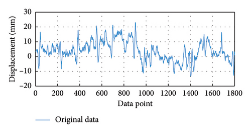
To evaluate the applicability of the proposed method, this section conducts supplementary research using the longitudinal displacement monitoring data. These data originate from Measurement point 11 at the L/2 position on the upstream side of the main bridge midspan, as presented in Figure 3. Data were collected at a 1 Hz sampling rate, with a total of 1800 points collected after December 24, 2023, at 12:00 p.m. The data distribution is displayed in Figure 17. In order to clearly illustrate the differences between the data of this experiment and the above experimental data, Table 20 gives their statistical properties including Max., Min., Std., avg., kurtosis (Kurt.), and skewness (Skew.). It can be observed that the attributes of the two datasets exhibit evident distinctions. This ensures the rationality of validating the practicality of the proposed method. In this experiment, the complete data are {x₁, x₂, …, x₇₂₀} and the missing data are {x₇₂₁, x₇₂₂, …, x₁₈₀₀} with a missing rate of 60%. The dataset is split into training, validation, and testing sets at proportions of 0.3, 0.1, and 0.6 [49]. Those sets are {x₁, x₂, …, x₅₄₀}, {x₅₄₁, x₅₄₂, …, x₇₂₀}, and {x₇₂₁, x₇₂₂, …, x₁₈₀₀}, respectively.

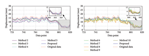
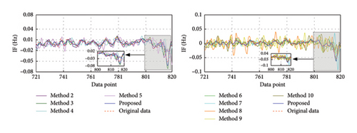
The training and validation sets are decomposed using SVMD, and a total of four IMFs are obtained. Each IMF is treated as a dataset separately and the corresponding TCN–MHA–BiGRU model is built for training and prediction. The recovered data are obtained by linearly superposing each IMF recovery result. Figure 18 displays the results for the proposed method and the other methods, with the corresponding evaluation metrics and training time provided in Table 21. The rate of change regarding evaluation metrics for the proposed method relative to other methods is displayed in Table 22. Evaluation metrics comparisons are shown in Figure 19.

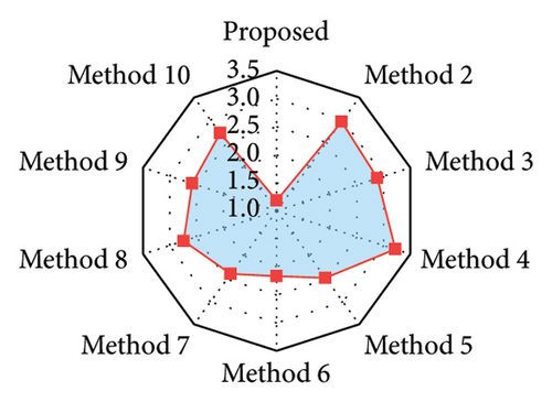
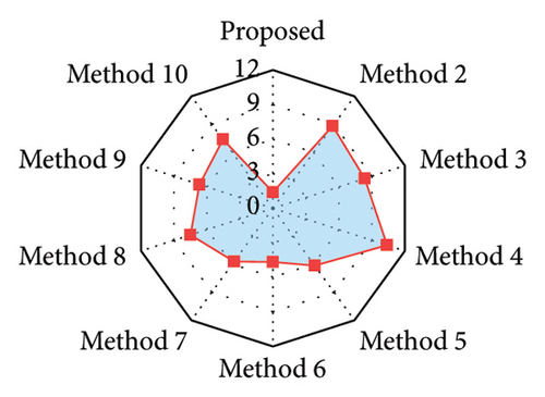
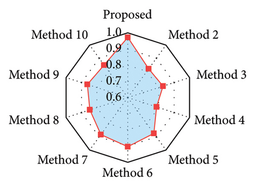
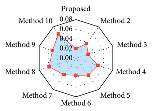
The observations in the following stem from the results analysis: (1) the SVMD-based method exhibits higher time-frequency recovery accuracy in comparison with those methods combining traditional signal decomposition techniques. (2) Among those methods without signal decomposition techniques, the TCN–MHA–BiGRU model significantly improves the recovery accuracy relative to other models despite the higher computational complexity (3) The proposed method (i.e., the combination of SVMD and TCN–MHA–BiGRU) consistently outperforms other methods in time-frequency recovery.

7. Conclusion

Despite the promising results achieved by the proposed method, the following aspects need to be further explored. (1) Develop more efficient deep learning models to realize the trade-off between performance and computational complexity. (2) Investigate the correlation among signals from different measurement points for improving the recovery accuracy. (3) Supplement the analysis of the probabilistic analysis of recovery results and the examination of anomalous data for further enhancing the recovery reliability. In addition, this study only focuses on the recovery of the monitoring data in the bridge health monitoring system. Future work can extend this method to other fields, such as solar radiation data and network traffic signals.

Conflicts of Interest

The authors declare no conflicts of interest.

Funding

The supports by the National Natural Science Foundation of China (Grant nos. 52108475 and 52278292), the Chongqing Outstanding Youth Science Foundation (Grant no. CSTB2023NSCQ-JQX0029), the China Postdoctoral Science Foundation (Grant no. 2023M730431), the Special Funding of Chongqing Postdoctoral Research Project (Grant no. 2022CQBSHTB2053), and the Science and Technology Project of Guizhou Department of Transportation (Grant no. 2023-122-001) are greatly acknowledged.