Explainable Artificial Intelligence–Based Search Space Reduction for Optimal Sensor Placement in the Pipeline Systems of Naval Ships
Abstract
Pipeline damage in mission-critical systems, such as pipelines within naval ships, can result in substantial consequences. Compared to manual inspection of pipeline damage by crew members onboard, structural health monitoring of pipeline systems offers prompt identification of damage sites, enabling efficient damage mitigation. However, one challenge of this approach is deriving an optimal sensor placement (OSP) strategy, given the large and complex pipelines found in real-scale naval vessels. To address this issue, a search space reduction method is proposed for OSP suitable for the large and complex pipeline systems found in naval ships. In the proposed method, the original search space for sensor placement is reduced to a manageable scale using an explainable artificial intelligence (XAI) technique, namely, a gradient-weighted class activation map (Grad-CAM). Grad-CAM enables quantification and visualization of the contribution of individual pipeline nodes to classify damage scenarios. Noncritical sensor locations can be excluded from the candidate search space. Furthermore, a peak-finding algorithm is devised to select only a limited number of nodes with the highest Grad-CAM values; in this research, the algorithm is proven effective in reconstructing the search space. As a result, the original OSP problem—which has an extremely large search space—is reconstructed into a new OSP problem with a computationally manageable search space. The new OSP problem can be solved using either meta-heuristic methods or exhaustive search methods. The effectiveness of the proposed method is validated through a case study on a real-scale naval combat vessel, measuring 102 m in length and carrying a full load of 2300 tons. The results show that the proposed XAI-based search space reduction approach efficiently designs an optimal pipeline sensor network in real-scale naval combat vessels.
1. Introduction
Pipeline damage in safety-related and mission-critical systems can result in substantial losses. To avoid such incidents and mitigate their consequences, structural health monitoring (SHM) has been implemented for various pipelines in engineering assets, such as petrochemical plants, power plants, ships, and buildings. The smart valves that the US Navy developed to enable prompt response to pipeline damage on combat vessels are an excellent example of SHM [1]. Recently, automated pipeline diagnostic systems on naval vessels have also been studied with the aims of (1) ensuring efficient mitigation of damages and (2) reducing the number of crew members needed onboard [2, 3]. Optimal sensor placement (OSP) is required to successfully implement SHM in the large and complex pipelines found on naval ships. If OSP is not performed properly (i.e., if the number of sensors is insufficient and/or the sensors are not placed at critical locations), the SHM outcome can suffer from fault-detection errors caused by unoptimized data acquisition. Thus, the SHM approach cannot produce the desired level of target detectability [4].
Numerous OSP studies were conducted to improve optimization algorithms [5], evaluation criteria [6], and frameworks [7, 8]. Enhanced optimization algorithms were actively studied. The OSP problem can be treated as an NP-hard problem in the mixed integer nonlinear programming (MINLP) form, while evolutionary algorithms (EAs) are suitable for solving OSP problems. To this end, variants of standard EAs were developed by introducing new encoding techniques [9], modifying the fitness function [10], and devising new operators [11–13]. Among them, genetic algorithms (GAs) have become a widely accepted approach.
Selecting sensor types and evaluation criteria are important in developing OSP procedures. In structural systems, modal information is widely employed. For example, modal analysis-based information entropy, the modal assurance criterion, and modal shape reconstruction methods are employed to evaluate the performance of sensor configurations [14–17]. On the other hand, it is limited to directly employ the evaluation criteria in pipeline structures that transport fluids. Damage detection methods for pipelines can be classified into exterior, visual, and interior methods, along with numerical approaches. Among these methods, it was reported that only interior methods, including mass-volume [18, 19] and pressure data [20–22], can cover a large system area [23]. Therefore, this paper adopts an interior method based on pressure data, combined with a numerical approach.
This study devises a search space reduction method suitable for OSP in the large and complex pipeline systems found on naval ships. As mentioned, most existing OSP-related studies focused on two aspects: (1) optimization algorithms and (2) evaluation criteria. However, conventional methods are limited in addressing the curse of dimensionality. The required sensor number increases exponentially with higher detectability targets, resulting in numerous local minima and elevated computational costs. Furthermore, GA approaches face challenges in sensor network design as their solution quality and computational efficiency decline in extremely large search spaces. They also lack effective guidance for relocating sensors when physical constraints make placement infeasible. To this end, the proposed method introduces a significant shift in focus by addressing the search space where optimization algorithms identify optimal sensor locations. Specifically, a novel framework was proposed by incorporating an additional phase, search space reduction, before the optimization phase. This innovation leverages explainable artificial intelligence (XAI) to determine critical sensor locations, effectively excluding nonessential regions from the original search space (OSS). By reconstructing the OSS, optimization algorithms can achieve the optimal sensor locations with improved efficiency and solution quality. Moreover, the application of XAI provides engineers with crucial insights into pipeline regions for damage detection, allowing them to refine sensor placement when physical constraints make the optimal design infeasible. In particular, the artificial intelligence (AI) model proposed in this study enhances the explainability of AI, making it easier for engineers to interpret and use critical information related to sensor placement. In this study, we demonstrate the effectiveness of the proposed method by applying it to the pipeline system of a real-scale naval combat vessel, measuring 102 m in length and carrying a full load of 2300 tons.
The remainder of this paper is organized as follows: Section 2 presents the challenges inherent in the sensor network design for studying the large and complex pipelines found in naval ships. Section 3 describes the proposed method. Section 4 presents a case study that was examined to validate the effectiveness of the proposed method. Finally, Section 5 concludes this paper.
2. Challenges in Sensor Network Design
This section provides an overview of the target system considered in this study. Then, the OSP challenges associated with the large pipelines found in the target system are briefly summarized, followed by a literature review.
2.1. Pipelines in Naval Ships
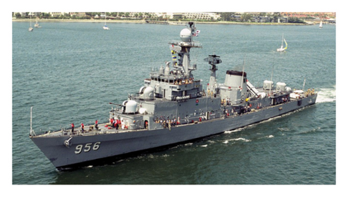
The naval ship examined in this study is an future frigate experimental (FFX) Batch-II, as shown in Figure 1(a). The vessel has a full load displacement of up to 2300 tons. It measures 102 m in length and has a beam width of 11.5 m. The vessel accommodates a crew of 150 personnel. Additional details are not disclosed for national security reasons. A drawing of a single section of the pipeline system of the naval ship is depicted in Figure 1(b) [11]. For this study, a testbed was built to emulate the hydraulic behavior of the pipeline subsection of a naval ship; this testbed and its simulation model of a single section with 109 nodes are shown in Figure 1(c). The simulation model was built using EPANET, an open-source software developed by the US Environmental Protection Agency (US EPA). The simulation model, which represents the pipeline subsection of the entire system, was initially designed to evaluate the feasibility of applying the OSP procedure in a prior study [11]. Details of this model can be found in the referenced study. In this paper, the simulation model shown in Figure 1(c) is utilized to aid in the understanding of the proposed method.
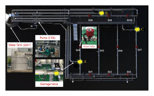
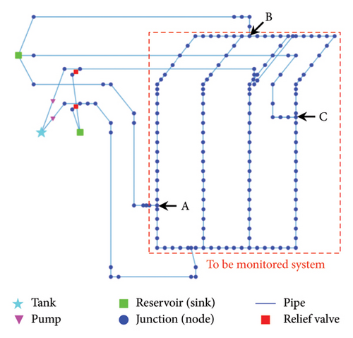
The simulation model inputs include the pipeline geometry, hydraulic parameters (e.g., minor loss and roughness coefficients), and pump specifications. The simulation model with calibrated parameters is employed to predict the hydraulic behavior of the main fire pipeline, such as the pressure and flow rate, under the assumption of pipeline damage due to ruptures. The damage scenarios (DSs) were predefined by domain experts. For instance, a pipeline rupture can result from a missile attack on the front, deck, or stern of a naval ship, corresponding to Sites A, B, and C in Figure 1(b). The scenarios “No damage” and damage at Sites “A,” “B,” or “C” were designated as DSs 1, 2, 3, and 4, respectively. If the pipeline is damaged by rupture, the water is drained out, resulting in a pressure drop from an initial high pressure (9 bars) to the atmospheric pressure.
The simulation model, accounting for measurement uncertainty and the inherent randomness of fluidic coefficients, can predict pressure data for given DSs. However, it is challenging to directly measure uncertain parameters, such as the minor loss and roughness coefficients, since an experiment using real-scale naval ships is infeasible. Therefore, in this study, the uncertain parameters are estimated using the hydraulic values measured from sensors on the testbed, which emulates one section of the pipeline system in a real-scale naval ship. Details on the calibration and validation of the simulation model can be found in the previous work of Kim et al. [11].
2.2. Problem Statement
Two-step approaches have been implemented to enable OSP to cope with the challenges posed by large structures with thousands of degrees of freedom [5, 24]. In the two-step approach, a reduced-order model is constructed first by capturing the essential dynamics of the large structure; this first step decreases the fidelity of the original structure and thus mitigates the computational burden [25–27]. For example, Casciati and Casciati [28] designed the control law based on a reduced-order model in the wind-excited bridge. The reduced-order model has proven effective for OSP in large-scale structures, such as high-rise buildings, irregularly shaped towers, and cable-stayed bridges. Sun and Büyüköztürk [29] built reduced-order models of large structures, including a 21-story building and the 610-m high Canton Tower. Cao et al. [30] reconstructed full-field dynamic responses using a set of basic vectors obtained from high-fidelity data. The results demonstrated that the proposed method is both efficient and practical. However, unlike the large structures discussed above, reduced-order models are not available for naval ship pipeline systems. The large and complex pipelines of naval ships still require a full-blown numerical analysis to predict their complicated system behavior.
3. Proposed Method
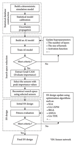
This section presents a procedure for a sensor network design with search space reduction by the XAI technique [31, 32]. A flowchart of the proposed method for the sensor network design is shown in Figure 2. First, a statistical database is constructed using a simulation model that emulates the hydraulic behavior of the pipeline system. Then, a convolutional neural network (CNN) model is trained on this database while optimizing its hyperparameters. After validating the CNN model, Grad-CAM values are computed to exclude noncritical sensor locations from the candidate search space. Consequently, the original OSP search space is reconstructed using only the remaining critical sensor locations. Finally, a meta-heuristic method is employed to select optimal sensor locations in the reduced search space (RSS) while ensuring target detectability.
3.1. Statistical Database Construction
Sensor data are required to develop a data-driven fault-diagnostic model for pipeline systems. The hydraulic simulation model is built and calibrated using the small-scale testbed’s experimental data. After calibration, it is assumed that the simulation model can emulate the target pipelines in real-scale naval ships. More information can be found in the previous publication by Kim et al. [11].
A statistical database is constructed using the Latin hypercube sampling method with a calibrated simulation model. A pair of inputs and corresponding outputs are recorded as a single datum. A statistical database is constructed by accumulating individual data. The statistical database contains values for the roughness coefficient, minor loss coefficient, measurement error, and pressure drops. For training and testing CNN models in pipeline fault diagnosis, the statistical database is divided into training and test sets.
3.2. Search Space Reduction
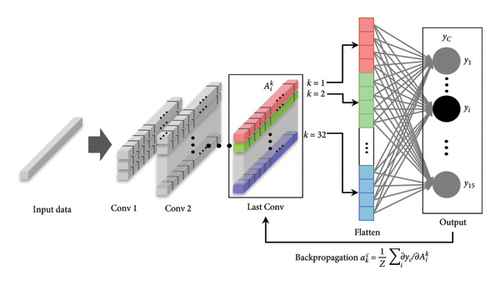
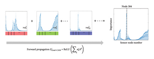
The proposed CNN model is trained to classify the DSs using the statistical database. The hyperparameters of the CNN model, such as the number of layers, kernel size, and activation function, are optimized so that the detectability is maximized. Figure 3(b) illustrates how to compute Grad-CAM values. The Grad-CAM values indicate the contribution of individual sensor nodes at the convolutional layer for the predicted class. Therefore, Grad-CAM values are used to reconstruct the OSS into a reduced one that only includes critical sensor locations for classifying DSs.
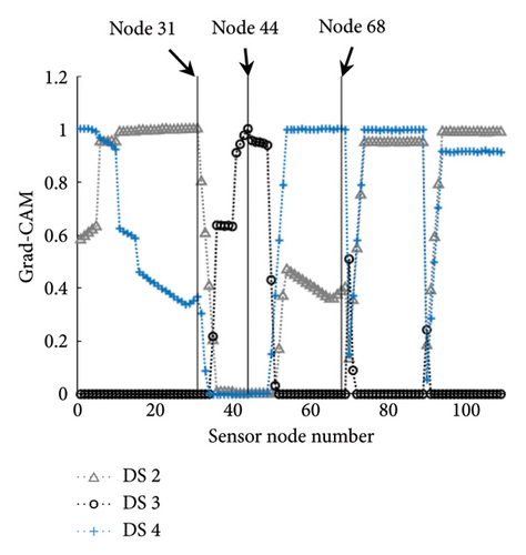
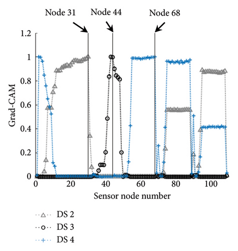
The contributions of individual sensor locations to classify DSs are calculated using the Grad-CAM values. For example, the Grad-CAM values of the small-scale testbed are presented with three DSs, as shown in Figure 4. In Figure 4(a), Nodes 31, 44, and 68 have the highest peaks of Grad-CAM values for DS 2, DS 3, and DS 4, respectively. This indicates that the three nodes offer the most critical information for classifying the DSs. When the CNN model has a recursive-softmax layer, the difference in Grad-CAM values between sensor nodes increases, as shown in Figure 4(b). The Grad-CAM values at the three nodes have sharp peaks compared to those shown in Figure 4(a). Thus, it is verified that the proposed CNN model with the recursive-softmax layer effectively visualizes the sensor location contribution for given DSs.
Grad-CAM values are distributed with a peak value at a particular region. Including all the nodes in a single region as candidates for a RSS is unnecessary. Instead, finding several candidates in multiple regions effectively maximizes the detectability. To this end, a peak-finding algorithm (PFA) is devised to select a small number of nodes with the highest Grad-CAM peaks in individual DSs. This algorithm identifies sensor nodes with peak Grad-CAM values. The pseudo-code for the algorithm is described in Algorithm 1. The PFA is executed repeatedly for all DSs to select critical nodes based on Grad-CAM values, classifying the given DSs.
-
Algorithm 1: Peak-finding (D, np, bd).
-
Require: One-dimensional Grad-CAM data D, the number of peaks np, the bounds of distance from selected nodes bd
-
Collect peak nodes and sort based on the Grad-CAM values: Dsort ⟵ sort (D)
-
Initialize iterator: t ⟵ 1
-
Initialize selected nodes: Dsel≔[]
-
while length(Dsel) < np do
-
Select nodes with the highest peak of Grad-CAM value: Dsel ⟵ [Dsel, Dsort[t]]
-
Check the constraint:
-
If (all index in Dsel—t) < bd:
-
t ⟵ t + 1
-
Else:
-
Select node indexed by t: Dsel⟵[Dsel, Dsort[t]]
-
t ⟵ t + 1
-
end if
-
Return Dsel
The PFA has two hyperparameters. First, the number of nodes to be selected (np) corresponds to the required nodes for each DS. Choosing a large value of np diminishes the effectiveness of the search space reduction, whereas choosing a small value of np can exclude potentially effective sensor locations. Thus, a tradeoff is required to select a proper value of np. Based on the authors’ experience, np should be chosen considering the total number of candidate sensor locations. For example, when np was set to 2, 3, and 4, the number of peak nodes increased to 5, 7, and 9, respectively, with two additional nodes added for each increment of np. Smaller np values reduce computational costs. However, they can eliminate critical sensor locations for damage classification. Gradually increasing np improves the likelihood of including the critical sensor locations. Thus, this study recommends starting with a smaller np and incrementally increasing it while verifying compliance with the target detectability. We set np to 3 in this study. Second, the bounds of the distance (bd) are used to avoid selecting already-selected sensors. The bounds of the distance are associated with the size of the convolutional operation kernels in the CNN model. During CNN model training, information regarding nodes is aggregated by the convolutional operator since the kernel size of the CNN model determines the node quantity. Therefore, the Grad-CAM values already include node information as the kernel size. In this study, bd is set as the kernel size to avoid selecting redundant information from neighboring nodes.
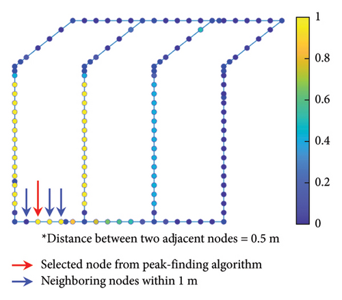
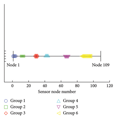
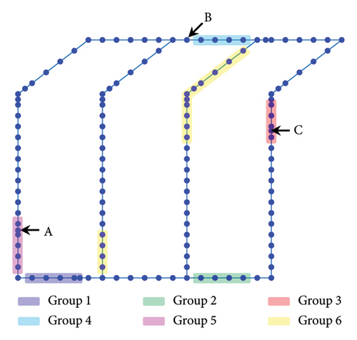
Using the nodes selected by the PFA, search space reconstruction is performed. The search space reconstruction comprises two steps: (1) adding neighboring nodes and (2) clustering. In the first step, physically adjacent nodes are incorporated with the existing ones. This step aims to reduce the discrepancy between Grad-CAM values and the physical locations of the corresponding sensor nodes. For example, the neighboring nodes within 1 m of the selected node were additively selected, as shown in Figure 5. Grad-CAM values are visualized through the node color. The higher the Grad-CAM values of nodes, the closer is to yellow, while lower values are represented by shaded closer to blue. In the second step, selected nodes are clustered using the density-based spatial clustering of applications with noise (DBSCAN) algorithm [35]. After the node groups are clustered, the empty spaces within individual groups are filled. Subsequently, clustered candidate node sets are selected. An illustrative example of the node index is presented in Figure 6. The final candidate nodes span the entire search space, ensuring comprehensive coverage (i.e., all design points). The total number of candidate solutions is expressed as Nn, where N represents the number of final candidate nodes, and the superscript n denotes the number of sensors used in the sensor network design. Six groups are clustered, and empty spaces for individual groups are filled. The individual groups consist of 1–4 (4 nodes), 11–14 (4 nodes), 28–31 (4 nodes), 41–44 (4 nodes), 65–69 (5 nodes), and 86–97 (12 nodes), respectively. Finally, 33 nodes are selected as the candidate sensor locations in total. A new RSS is constructed using the final candidate sensor nodes. The physical locations of the final candidate sensor nodes are described in Figure 7. Intuitively, one might assume that the damage points exhibiting the greatest pressure drops are the optimal locations for sensor installation. However, regions distant from the damage points (A, B, and C) are also included among the final candidate sensor locations. This suggests that classifying all DSs requires obtaining comprehensive information from multiple sensor locations.
3.3. Sensor Network Design
The sensor network design requires multiple iterations of classifying DSs using sensor measurements (e.g., pressure) to determine the sensor locations that maximize detectability. The sensor measurements are obtained by simulating the hydraulic model that produces a pressure distribution.
The OSP aims to find optimal sensor locations that maximize the evaluation criterion. To design a sensor network, the optimization problem is formulated in equation (6). This study employed detectability as the evaluation criterion. Detectability can be calculated using the PoD measure, which is the probability of the correct classification of detection of the classification algorithm [36].
The solution to the OSP problem can be found by implementing three steps. First, the number of sensors is set to be the lowest bound allowed in the optimization problem. Second, a search is conducted for a combination of sensor locations that exceeds the target detectability. If the target detectability is not achieved, the number of sensors is incremented by one. Last, the second step is repeated until the target detectability is achieved or the upper bound of the number of sensors allowed is reached. With the RSS discussed in Section 3.1, meta-heuristic methods such as GAs can be implemented to find the optimal solution. An exhaustive search will be feasible when the RSS is small, and the computational burden is tolerable.
4. Case Study
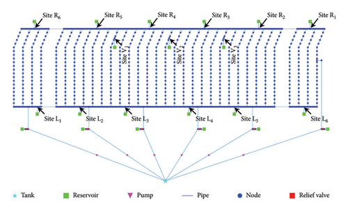
In this section, we move from the small-scale model presented in Figure 1(c) to the real-scale model of the pipeline system used in an FFX-Batch II naval combat vessel, as shown in Figure 8. The real-scale model is employed to verify the effectiveness of the proposed method. First, the implementation details of the proposed method are described. Then, the results are described, and a performance comparison is provided. Last, a discussion of the case study and its results are presented.
4.1. Implementation Details
The real-scale pipeline simulation in Figure 8 is approximately ten times larger than the small-scale pipeline system in the prior study [11]. As a result, the quantity of sensor nodes increased from 109 to 1026, all are potential locations for sensor placement. Fifteen failure sites were identified by domain experts, considering possible attacks from an enemy. Due to the increased number of potential failure sites, the number and complexity of possible DSs have likewise grown. Among them, ten DSs were simulated in this case study (i.e., no damage + nine combinations of damage sites).
The normal state without any damage was defined as DS 1. DSs 2 to 4 were defined as single damaged points at L2, R6, and R1. DSs 5 to 7 were defined with two damaged points in each scenario, at (R5, V3), (R2, R3), and (L2, L5), respectively. DSs 8 to 10 were set with three damaged points for each scenario, at (R2, R5, V1), (L1, L5, L6), and (L4, R1, V2), respectively.
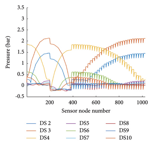
The nominal pressure values along the sensor node from the real-scale simulation model are shown in Figure 9. An optimal sensor location cannot be determined by visual inspection since the pressure distribution is too complicated. Moreover, the pressure values deviate due to measurement uncertainty and the inherent randomness of the pipeline systems. Therefore, an optimal sensor network should be determined by the systematic approach.
A statistical database was constructed using the real-scale simulation model. The dominant uncertainty sources of the simulation model were minor loss and roughness coefficients since the dominant factors affecting the hydraulic flow in a pipeline are corrosion and turbulence. Measurement errors induced by the variability in measurements were incorporated into the model. The pipe’s roughness and minor loss coefficients were modeled as normal distributions, N(0.05, 0.005) and N(150, 15), respectively [37, 38]. The mean value for the roughness coefficient was determined based on the material (i.e., stainless steel) used in our experiment. The mean value of 150 for the minor loss coefficient was selected considering the bends in the designed pipeline system. The standard deviations were set to have a coefficient of variance of 0.1 [39, 40]. The measurement error was assumed to follow a normal distribution N(0, 0.0138). As reported in [3], the standard deviation of the measurement error was characterized through repeated pressure measurements using a prototype nonintrusive sensor system. Uncertainty propagation was conducted via a Monte Carlo sampling method, with 10,000 data samples generated for each DS. A statistical database was constructed using pressure data from 90,000 data samples along the pipeline for the nine DSs, excluding the normal state. Of the total database, 80% was allocated for training, and the remaining 20% was reserved for testing. In summary, the datasets for the individual DSs were divided into training and test data with 72,000 and 18,000 data samples, respectively.
A CNN model was built to classify the DSs for the real-scale pipeline system. The architecture of the CNN model is shown in Table 1. The input was the pressure values of the 1026 nodes from the simulation model, while the output was one of the nine DSs. DS 1 was excluded from the classification task since the pressure value for the normal state was evident (i.e., 9 bars throughout the pipeline). The grid-search method optimizes the hyperparameters of the CNN model, such as the number of layers, kernel size, and activation function. The CNN model was trained to classify the nine DSs. A validation accuracy of 100% was achieved during the training process. It is important to recall that the objective of building the CNN model is to calculate the Grad-CAM values.
| Layer | Output shape | Number of parameters | Note |
|---|---|---|---|
| Input layer | (None, 1,026, and 1) | 0 | — |
| Convolutional layer 1 | (None, 1,026, and 8) | 96 | Kernel = 5; filter = 16 |
| Convolutional layer 2 | (None, 1,026, and 16) | 544 | Kernel = 1; filter = 32 |
| Recursive-softmax layer | (None, 1,026, and 16) | 0 | — |
| Flatten layer | (None, 32, and 832) | 0 | — |
| Output layer | (None and 9) | 295,497 | — |
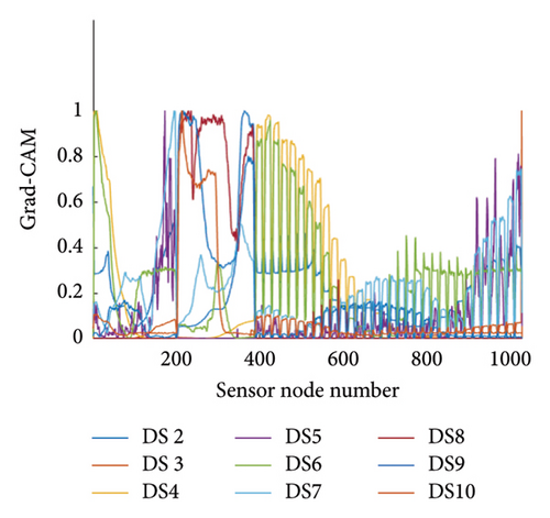
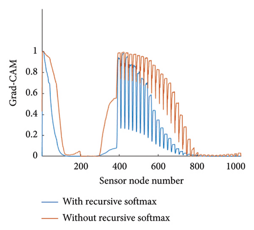
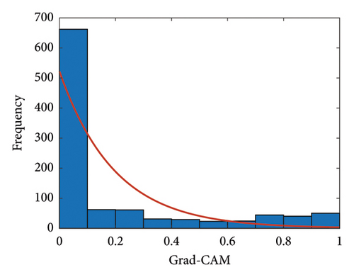
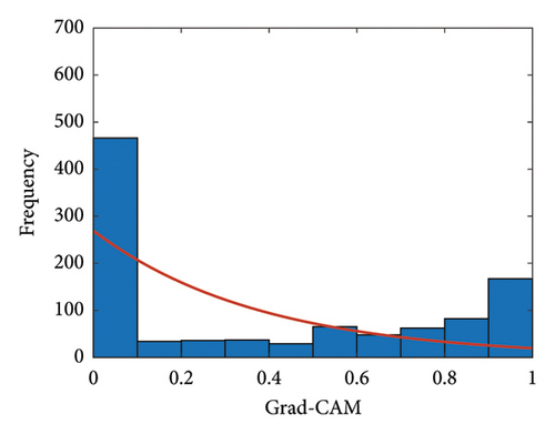
The contribution of the sensor locations to damage classification was calculated using the Grad-CAM technique. The Grad-CAM results of the real-scale pipeline system for all DSs are described in Figure 10(a). The horizontal axis indicates the sensor node number, and the vertical axis indicates the Grad-CAM values. The individual lines present the contribution along the sensor node number for individual DSs. For this case study, the effect of the proposed model with the recursive-softmax layer is compared with that of a conventional CNN model without the recursive-softmax layer. As a representative example, the Grad-CAM values of DS 4 are shown in Figure 10(b). As expected, the Grad-CAM values from the CNN model with the recursive-softmax layer showed sharp peaks compared to the results without the recursive-softmax layer. The effectiveness of the proposed model with the recursive-softmax layer can be analyzed statistically. When two individual Grad-CAMs are fitted to the exponential distribution, the individual hyperparameters (λ) are estimated as 0.19 and 0.38, respectively. The distributions of the Grad-CAM values with/without the recursive-softmax layer can be graphically compared, as shown in Figures 10(c) and 10(d). The proposed method yields the Grad-CAM distribution that tends to lean toward zero values. Consequently, it can be inferred that the proposed model better emphasizes the highlighted Grad-CAM values than the conventional CNN model.
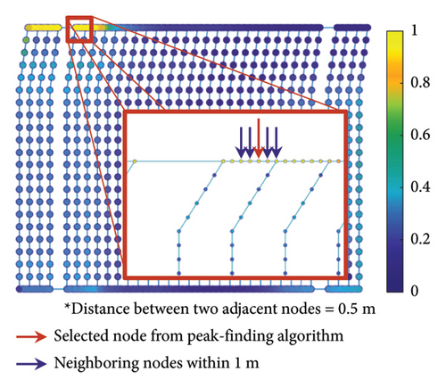
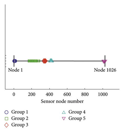
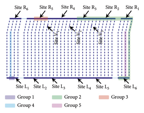
The PFA was used to determine the sensor nodes that exhibit the highest Grad-CAM peaks. The parameters of the PFA, including np and bd, were set to three and five, respectively. As a result, 22 peaks were identified by the PFA across all DSs. The search space was reconstructed in two steps. In the first step, neighbors within 1 m of the peaks were added as candidate sensor locations, as illustrated in Figure 11. The Grad-CAM values indicated by the color at the node are between zero and one. The yellow color indicates that Grad-CAM values are closer to one, while the blue color represents that the Grad-CAM values are closer to zero. The sensor node indicated by the red arrow is determined by the PFA, while the sensor nodes indicated by blue arrows are neighboring nodes within 1 m of the peak node. It should be noted that the distance between adjacent nodes is 0.5 m. Consequently, the number of candidate sensor nodes increased from 22 to 97. In the second step, 97 sensor nodes were clustered using the DBSCAN algorithm, and individual clustered groups were filled out to eliminate any empty spaces. The 97 sensor nodes were clustered into five groups, and individual groups were filled without any missing nodes, resulting in a final count of 171 candidate sensor nodes. The sensor nodes within individual groups consist of 5–13 (9 nodes), 172–279 (108 nodes), 334–355 (22 nodes), 411–426 (16 nodes), and 1011–1026 (16 nodes), as shown in Figure 12. The physical locations of the final candidate sensor groups are illustrated in Figure 13. Among 15 candidate damage points, five (L6, R1,2,3,5) are included in candidate sensor groups, while 10 locations are excluded. The counterintuitive observation can be explained by the assumption that the AI classified all DSs simultaneously rather than individually.
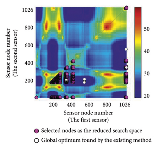
The original and RSSs are visualized in Figure 14, where two sensors are employed. The horizontal and vertical axes indicate the sensor node number of the first and second sensors, respectively. The color of the heat map represents the objective function values (i.e., fitness), and magenta circles illustrate the candidate sensor combinations. In the proposed method, the optimization algorithm explores only the RSS, which is only 2.76% (14,535/525,825) of the OSS. For the case of three sensors, sensors within three groups are combined; thus, the total number of sensor combinations becomes 818,805. The size of the OSS is 179,481,600 when three sensors are employed. Therefore, a search space reduction of 99.54% is achieved in the second case.
4.2. Results
Optimal sensor networks were designed using the proposed method. The optimization procedure was conducted by increasing the quantity of sensors until target detectability was achieved. In this study, the desired level of target detectability was determined to be 99%. The results of OSP using the proposed search space reduction method are summarized in Table 2. To consider the probabilistic nature of the meta-heuristic algorithm, 30 optimizations were performed, and the detectability and computational costs were determined using the average values. As expected, as more sensors are employed, the detectability also increases. Finally, the target detectability of 99% was achieved using 20 optimal sensor locations with a computational time of 3819.2 s.
| Sensor quantity | Computational costs (seconds) | Sensor locations | Detectability (%) | |
|---|---|---|---|---|
| Search space reduction | Optimization | |||
| 1 | 16.0 | 76.6 | (342) | 65.9 |
| 2 | 90.6 | (174, 346) | 83.1 | |
| 3 | 132.2 | (175, 178, 347) | 86.7 | |
| … | … | … | … | |
| 19 | 199.5 | (174, 182, …, 1025) | 98.9 | |
| 20 | 236.1 | (174, 178, …, 1025) | 99.0 | |
| Total | 3819.2 | — | — | |
The effectiveness of conducting OSP in RSS against OSS was evaluated. For this purpose, the existing state-of-the-art (SOTA) meta-heuristic methods were implemented in RSS and OSS. Table 3 shows five SOTA optimization algorithms, including GA-LXPM (SGA in MATLAB; GA with Laplace crossover and power mutation), discrete artificial bee colony algorithm (DABC), Adam-mutated GA (AMGA), improved real-coded GA (IRGA), and GA-two direction crossover (GA-TDX). The OSP results are summarized in Table 4. Due to the proposed search space reduction method, the number of sensors required to achieve target detectability (i.e., 99%) decreased. The results indicate that higher detectability can be attained when the same number of sensors is given. Therefore, it is corroborated that the proposed method improved solution qualities for all individual SOTA optimization algorithms. For example, in the case of SGA, the number of employed sensors to achieve the target detectability of 99% was reduced from 25 to 20 (−20%). With DABC, only 18 sensors (−5.3%) were required in the proposed method, while 19 were employed using the conventional OSP approach (i.e., no use of the search space reduction). The improvement in solution qualities is explained graphically in Figure 15. The required sensor quantity was reduced in the proposed method for all cases against the conventional OSP without search space reduction.
| Optimization algorithm | Crossover operator | Mutation operator | References |
|---|---|---|---|
| Genetic algorithm with Laplace crossover and power mutation (SGA; GA-LXPM) | Laplace crossover | Power mutation | [41, 42] |
| Discrete artificial bee colony (DABC) | Employed bee, onlooker bee, and scout bee | [29] | |
| Improved real-coded genetic algorithm (IRGA) | Directional crossover | Directional mutation | [43] |
| Adam-mutated genetic algorithm (AMGA) | Laplace crossover | Adam mutation | [11] |
| Genetic algorithm with two-direction crossover (GA-TDX) | Two-direction crossover | Grouped mutation | [44] |
| Algorithm | Sensor quantity | Computational costs (seconds; included search space reduction cost) | ||||
|---|---|---|---|---|---|---|
| OSS method | RSS method (proposed) | Decreased expense (%) | OSS method | RSS method (proposed) | Decreased expense (%) | |
| SGA | 25 | 20 | −25.0 | 6255.2 | 3835.3 | −38.7 |
| DABC | 19 | 18 | −5.3 | 8639.9 | 6580.3 | −23.8 |
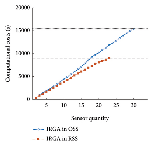
| IRGA | 33 | 23 | −30.3 | 15,410.0 | 9029.0 | −41.4 |
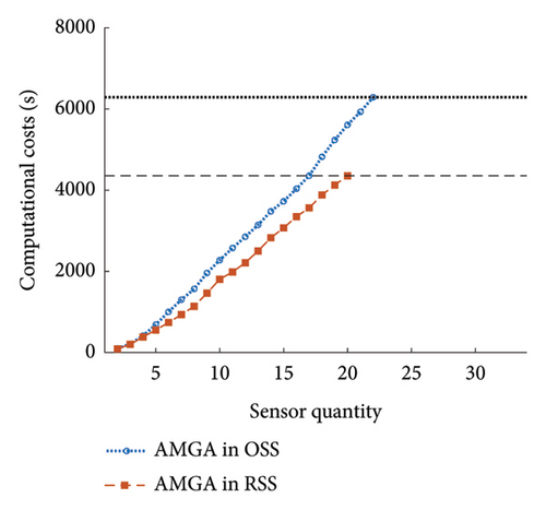
| AMGA | 22 | 20 | −9.1 | 6290.2 | 4371.2 | −30.5 |
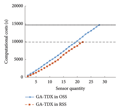
| GA-TDX | 28 | 22 | −21.4 | 14,700.1 | 9901.5 | −32.6 |
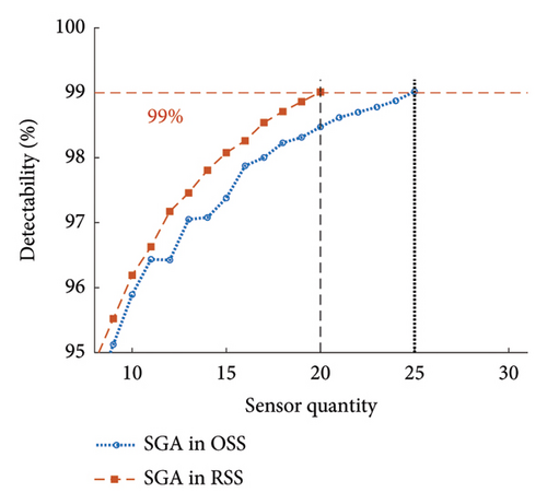
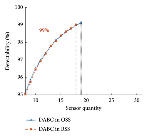
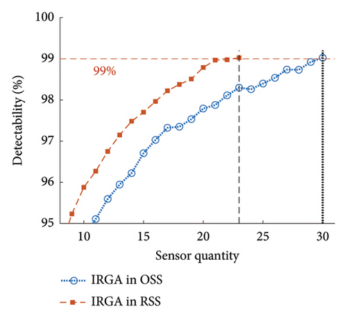
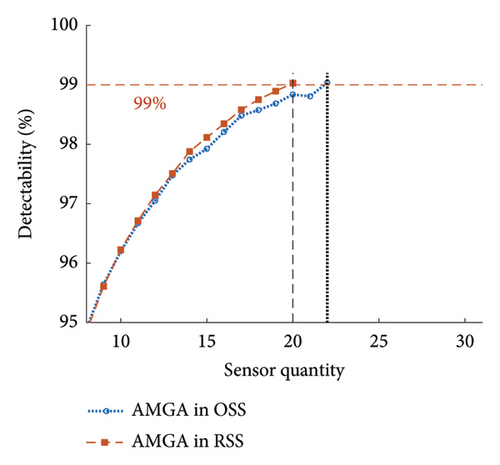
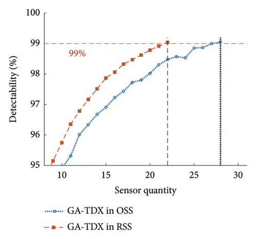
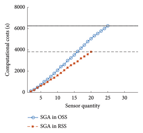
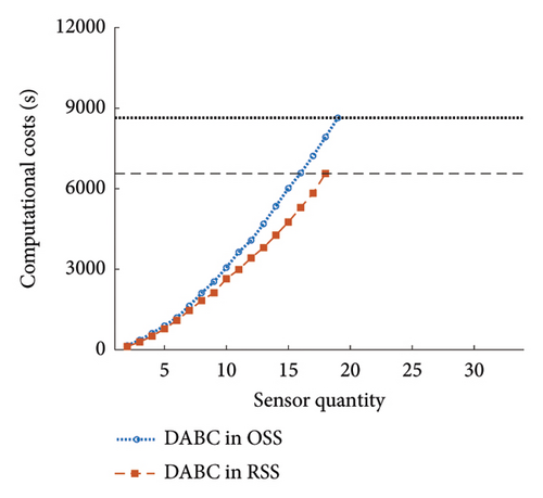
The effectiveness of the proposed method was also observed in the aspect of efficiency. For all cases, the computing time decreased by at least 23.8%. The enhanced efficiency can be explained using the accumulative computational costs shown in Figure 16. First, the number of total OSP trials was reduced. Due to the improvement in solution qualities, the target detectability was achieved with fewer sensors. For example, five additional OSP trials were saved using the proposed method in the SGA case. Second, the computing time in a single OSP procedure was reduced. The slope of accumulative computational costs in Figure 16 indicates that the optimization algorithms can return the optimal solution faster in RSS than in OSS. Therefore, both aspects of sensor quantity and efficiency contributed to the lower computational costs in the overall procedure of OSP.
4.3. Discussion
The proposed method offers the flexibility of relocating sensors by visually inspecting the Grad-CAM image of the pipelines when sensor placement at the optimally designed locations is not feasible due to physical constraints at the specified locations. As shown in Figure 11, the sensor can be relocated manually by visually comparing the Grad-CAM values when a sensor cannot be placed at the optimally selected node. If GA-based methods are used, this option (the relocation of sensors) will not be available since no information near the optimally selected nodes is provided. If sensor relocation becomes necessary, the calculation must be repeated after excluding the problematic sensor location, significantly increasing the computational burden. In fact, noncritical sensor locations can be excluded before finalizing the solution. In such cases, there is no significant difference between conventional methods and our proposed approach. However, if engineers encounter infeasibility in sensor placement due to physical constraints, our proposed approach offers an efficient guideline for relocation. Unlike conventional methods, which require repeating the optimization process, our approach enables engineers to make faster decisions using the Grad-CAM value distributions, highlighting optimal areas for sensor placement. Thus, the proposed framework facilitates easy adjustment of sensor locations, minimizing trial and error.
It is important to note that the proposed method is not limited to the OSP of naval ships. The key idea, namely, XAI-based search space reconstruction, can be extended to the large, complex pipeline systems of other engineered assets. The result could be a significant reduction in the required sensors without compromising the target detectability. For those applications (such as petrochemical plants), the costs of initial sensor installation, data acquisition and processing, and big data analytics can be critical for the successful implementation of SHM.
5. Conclusions
This study proposed a novel framework for OSP in a large, complex pipeline system. Compared to the existing framework, the proposed framework that combined the SSR method with XAI was never reported in the literature. Previous studies have focused on enhancing individual components within the existing OSP frameworks, such as improving optimization algorithms or evaluation criteria. In contrast, this study introduces a novel framework incorporating an entirely new phase (i.e., SSR) alongside the conventional phases. This sets our approach apart because, unlike other methods that require replacing existing components, our proposed method can be seamlessly integrated into the existing OSP framework without removing or substituting the components. In doing so, it enhances the effectiveness of the original framework, yielding improvements in both solution quality and computational efficiency.
To account for the expansibility of the proposed method, the performance of the proposed framework was evaluated using SOTA GAs in the RSS, including GA-LXPM, DABC, AMGA, IRGA, and GA-TDX. It was found that the proposed framework improved both solution quality and computational efficiency. The proposed framework offers a unique benefit: the flexibility of relocating sensors by visually inspecting the XAI images of the pipelines when sensor placement at the optimally designed locations is not feasible due to physical constraints at the specified locations. The key idea of the proposed framework using SSR by XAI has the potential for extension into other application domains beyond the OSP for naval ships, such as petrochemical plants and thermal power plants. Therefore, the proposed framework will benefit many researchers and industrial engineers.
The XAI technique (i.e., Grad-CAM) with the PFA was proposed to reconstruct the search space to design an optimal sensor network. For OSP, a combinatorial optimization problem was tackled to be solved using an exhaustive search. However, the computational cost was not manageable for large, complex pipeline systems such as naval ships. With advanced GAs, it was possible to obtain a sensor network design solution. However, the quality of the solution was not satisfactory. The proposed method significantly enhanced the quality of solutions from optimization algorithms. The sensor network design of pipeline systems was a multimodal problem in which numerous local minima exist. The proposed method effectively found an enhanced solution with even less computational time. The effectiveness of the proposed method was demonstrated in the case study of a real-scale pipeline system of an FFX Batch-II naval combat vessel. Using the proposed method, an optimal sensor network was designed to satisfy the target damage detectability of 99% with the reduced number of sensors compared with the existing methods. It is concluded that the proposed method can improve the solution quality when the same number of sensors is given.
This study focused on developing and validating a single-objective optimization framework for OSP, serving as a foundational step. However, it is limited in addressing practical scenarios involving multiple conflicting factors, such as information redundancy and coverage efficiency. Future work should extend the framework to a multiobjective optimization perspective, enabling the evaluation of tradeoffs between conflicting objectives. Incorporating additional indicators will enhance the framework’s adaptability to real-world applications and provide engineers with a comprehensive tool for OSP in complex systems.
Conflicts of Interest
The authors declare no conflicts of interest.
Funding
This work was supported by the National Research Foundation of Korea (NRF) Grant Funded by the Korea government (MSIT) (No. RS-2022-00144441, No. 2021R1A2C1008143, and No. 2021M2E6A1084687) and by the Basic Project of Korea Institute of Machinery and Materials (Grant no. NK244B).
Acknowledgments
This work was supported by the National Research Foundation of Korea (NRF) grant funded by the Korea government (MSIT) (No. RS-2022-00144441, No. 2021R1A2C1008143, and No. 2021M2E6A1084687) and by the Basic Project of Korea Institute of Machinery and Materials (Grant no. NK244B).
Open Research
Data Availability Statement
The data underlying the findings of this study are related to the naval vessel research in the Republic of Korea Navy. Due to sensitive military security concerns, the data cannot be made publicly available.


