The application of machine learning techniques in bridge health monitoring is gaining widespread popularity as it overcomes the problems faced by conventional methods. However, the scarcity of labeled data for damaged bridges in training the model acts as a hindrance. The present study proposes a data science–based novel approach for overcoming this hindrance using a semisupervised, output-only method for multiple-level damage identification of a steel truss bridge. The method employs sequence-to-sequence modeling of vehicle-induced vibration response only from a single sensor position. The authors have used a bidirectional long short-term memory (BiLSTM) network for damage feature extraction. A statistical distance metric tool, Kullback–Leibler divergence, has then been utilized for feature discrimination. The method’s efficiency is numerically investigated through a 3-D finite element model of a steel truss bridge based on real bridge specifications. A dynamic analysis using a moving vehicle is performed to obtain vehicle-induced accelerations. A total of 36 different damage scenarios have then been incorporated into the bridge. The effect of sensor position and performance because of variation in vehicle operation has also been investigated. The results show that the proposed approach successfully detects all the damage scenarios. The methodology’s performance has also been validated in detecting damages for the Old ADA Bridge benchmark data. The methodology successfully detected multiple damage states using a single sensor response.

1. Introduction

Smooth and unhindered communication is a prerequisite to ensure the economic growth of a country. Bridges are an essential infrastructure in ensuring such communication. These bridges usually have a long design life of about 120 years [1]. However, even before reaching the end of its design life, the service function of the bridge degrades under cracking, fatigue, corrosion, and other damage to the structure resulting from different geological hazards [2]. Such premature failure of the bridges may also be caused by discrepancies between the design and constructed structure, as well as unexpected traffic increases [3]. Thus, monitoring the bridge’s health is crucial to ensure its smooth functioning [4]. However, visual inspection of bridges is subjective, time-consuming, laborious, and prone to error [5]. In recent years, owing to improved and easy sensing technologies, this aspect of bridge health monitoring (BHM) has been easily accomplished via structural health monitoring (SHM) [6, 7]. SHM can be defined as an intricate system composed of sensors, data processing, modeling, and damage detection components [8]. Vibration-based SHM has been tested and proven to be a promising field in detecting bridge damage and monitoring the bridge’s condition [9–11]. The vibrational responses are analyzed in the time domain, frequency domain, and time–frequency domain for structural damage identification.

SHM data used to study the bridge’s condition comprise model-based and data-driven approaches. The model-based approach primarily used modal parameters, namely, damping, frequency, and mode shape, to detect damage in the bridge using SHM data. However, exciting higher modes required for identifying local damage involved in this approach are difficult. Moreover, the mode shape-based method is sensitive to measurement noise and variation in operation [12, 13]. The model-based approach requires developing a precise finite element model (FEM) of the structure in the pristine state, which is referred to as the baseline model. This FEM of the structure, which replicates the behavior of the actual structure based on the collected data, is called its digital twin [14]. The digital twin of the exact model requires calibration as the structure ages over time. Structural damage is detected by comparing the calibrated FEM to the baseline model. This approach has been applied to the SHM of different structures supplemented by statistical and signal processing techniques [15–18]. However, there is the problem of uncertainty and error in calibrating the model to be consistent with the damaged state of the structure. The calibration involves many parameters associated with high modeling costs, which could hinder performance [19]. To overcome these limitations, researchers are now focusing on data-driven algorithms.

The conventional data-driven approach relies solely on the measurements from the actual structure without requiring a physical model of the structure [20]. This approach uses an acceleration response from vehicle-induced bridge vibration, which provides an added advantage of damage detection for inaccessible locations and real-time application [21]. Deviations in the bridge response in the damaged condition from the response in the undamaged condition are then captured using various signal processing and statistical techniques to detect bridge damage [22]. Challenges in SHM created by operational variations [23] and multiple sensor requirements [22] faced by the conventional data-based approach can be circumvented using ML algorithms based on their powerful learning ability and high computational efficiency [24, 25]. Moreover, the operational variation may modify the modal properties of the structure, hindering SHM using a model-based approach, which can be overcome by implementing machine learning (ML) algorithms [26]. These techniques incorporate artificial intelligence (AI) to ensure minimal human intervention, thereby reducing costs and, at the same time, increasing reliability.

The ML approaches can be divided into three categories depending on whether a labeled or unlabeled dataset is used in the training process: supervised, unsupervised, and semisupervised. Of all the ML models, artificial neural networks (ANNs) have gained much attention in recent years [22]. Researchers have developed a vast array of ANNs. Multilayer perceptron (MLP) can have multiple hidden layers, with nonlinear activation functions within the multiple neurons in these layers. The weights are adjusted using backpropagation [27, 28]. MLP has shown significant success in its application to SHM of bridges in recent years [29–31]. However, its application to SHM data for vehicle-induced vibration is difficult because of the complex nature of the data and the inherent weakness of MLP in processing the data [22]. Deep neural networks (DNN) have also been used in the SHM of a calibrated FE model of a steel truss bridge where natural frequencies are mapped with the artificially induced damages (1%–50% stiffness reduction) in the FE model [31]. Based on the success of convolutional neural networks (CNNs) in image processing, it has also been applied to the supervised learning-based algorithm in SHM for detecting cracks and identifying damage using a vibrational response from structures [32]. Significant research has been done using CNN in SHM for crack detection of bridges and structures [33–37]. However, acquiring large volumes of images and preprocessing them to train the network remains a significant challenge, a major drawback of supervised learning-based algorithms.

Recurrent neural networks (RNNs) are a popular ML algorithm for time series data analysis because of their ability to retain historical information from the input sequence. RNN can be utilized in the bridge acceleration response analysis, as it is highly relevant to the time series data. However, conventional RNNs are susceptible to the vanishing gradient and exploding gradient problem [38]. This drawback of the conventional RNN can be overcome using gated units such as long short-term memory (LSTM) [39]. LSTM has been successful in predicting dynamic displacement [40] and structural response under the effect of wind [41], as well as bridge damage detection [42]. Based on the success of LSTM in SHM, damage detection has been expanded to BiLSTM for a numerical example, and the Z24 bridge uses artificial excitation with shakers [26]. However, all these studies are based on a supervised learning-based algorithm, which might not always be practical because of the lack of labeled data from the damaged structure to train the ML model. Based on the superiority of the BiLSTM model in BHM, the present study aims to detect damage in a steel truss bridge using a semisupervised learning-based algorithm where the bridge response only from the undamaged state is required. In addition, the method employs vehicle-induced response without the need for artificial bridge excitation.

1.1. Novelty of the Study

Recently, various techniques have been proposed for damage detection of steel truss bridges. Mustafa et al. [43, 44] have used modal damping and mode shapes as the damage-sensitive feature on an existing steel truss bridge. However, in real-life scenarios, the energy dissipation depends on the type of damage, and structures may not show purely viscous damping which may hinder the damage detection [44]. Studies have also been carried out on railway steel truss bridges for damage detection [26, 45, 46] using data-driven methods validated either on a FE model or a lab-scale model. In addition, these studies used white noise for bridge excitation instead of applying actual vehicle-induced vibration which is inherently complex because of its nonstationary nature. Nguyen-Ngoc et al. [31] used DNN with a new optimization algorithm for damage identification of a calibrated FE model of a steel truss bridge where natural frequencies are mapped with the artificially induced damages (1%–50% stiffness reduction) in the FE model [31]. Such type of labeled data for training the DNN model might not be feasible in real-life applications.

Riasat Azim and Gül [47] used the ARMAX time series model on bridge responses simulating a train passing over the calibrated FE model to obtain the damage-sensitive features. However, for the ARMAX model, the selection of appropriate parameters and models are crucial for result accuracy. The accuracy is also influenced by the model’s sensitivity to measurement noise. Moreover, special attention is required for nonstationary measurement signals [45]. In addition, the study used a damage severity level, with the lowest being 20%. Azim and Gül [46], in another study, used principal component analysis (PCA) of strain response for damage detection, which is numerically verified on the FE model of a railway truss bridge with added artificial noise. The method could identify damage induced by stiffness change, at least 20% to as low as 10%, depending on operational variability and measurement noise level. This indicates the sensitivity of the result accuracy of the PCA-based method to the level of random noise in measurement. Mousavi et al. [48] performed a damage detection approach based on empirical wavelet transform and ANN in a laboratory scale truss model subjected to white noise and impact excitation. The method was able to identify damage as low as 35% in the form of cross-section reduction. The included literature uses either FEM or lab-scale models to validate the methodology which may not be justified for practical applications. The unavailability of the real-world data from damaged bridges might have led to such an approach. However, the present study focuses on validation of the methodology using field experiment data.

Field experiments for SHM using vibration response have high reference values over FEM and laboratory tests, as they can replicate the operational conditions [21]. However, budget limitations and permission from relevant authorities to apply damage to a bridge to obtain vibration response present hindrances [21]. Some of the notable field experiments on the damage detection of real bridges are the Z-24 Bridge [49], Old ADA Bridge [50], I-40 Bridge [51], Dogna Bridge [52], and Alamosa Canyon Bridge. Chang and Kim [21] have conducted damage detection of the Old ADA Steel Truss Bridge using modal frequency, modal damping, modal assurance criteria (MAC), coordinated modal assurance criteria (COMAC), and their combinations as the damage-sensitive features, and Mahalanobis distance for feature discrimination [21]. For all the mentioned features, damage detection required data from multiple sensors, which could hinder SHM because of budget constraints. The methodology couldn’t discriminate between all the damage states using a single feature or their combinations, which would hinder its practical application because of the requirement of prior experience. In another study, Kim et al. [53] used Nair’s damage indicator (NDI) on a steel Gerber truss bridge for detecting a single damaged diagonal member. However, the methodology required a set of multiple sensors. In addition, all the sets of sensors were not successful in confirming the presence of damage. Data acquisition using a limited number of sensors is of utmost importance to ensure efficiency in damage detection. To overcome these hindrances, the authors have proposed a semisupervised learning-based algorithm using the response from a single bridge sensor. The proposed methodology is initially investigated through a numerical simulation based on the FEM of a real steel truss bridge. Further, the damage detection methodology was validated using the benchmark data for vehicle-induced vibration response of the “Old ADA Steel Truss Bridge.” The bridge response was collected from the studies available in the public domain [50, 54]. A single sensor response was used to detect damage for multiple damage states.

In this method, a sequence-to-sequence approach is utilized, where the input sequence generated from the response of a single sensor is used to predict an output sequence generated from the same response. The DL model uses a BiLSTM network with fully connected layers (FCLs). A FEM of an actual bridge has been developed. A dynamic analysis of the bridge is conducted to obtain the vehicle-induced dynamic response. The acceleration response from a joint in the bridge is used to evaluate damage. The DL network is trained for acceleration response incorporated with noise in the undamaged condition. The trained sequence-to-sequence model is referred to as the baseline model. Damage in the form of stiffness reduction is then induced into the horizontal members of the bridge. Deviations in the response predicted by the baseline model are captured. To confirm the presence of damage using the deviations in response, a statistical metric sensitive to the variation between the predicted response and the actual response is required. Past researchers have found Kullback–Leibler divergence (KLD) to be superior to other statistical approaches and PCA in responding to defects in complex dynamics systems [55]. In KLD-based damage detection, the current data are compared against reference data. KLD is utilized to discriminate the damaged state of the bridge and to confirm the presence of damage using a t-test.

2. Numerical Study

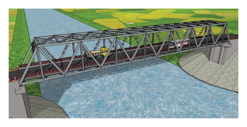
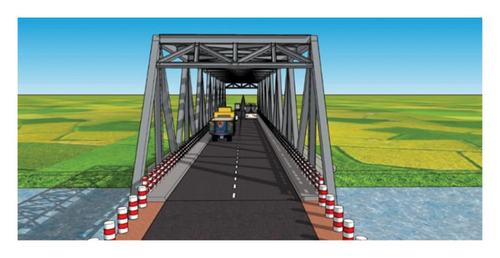
The present study aims to detect damage induced in a steel truss highway bridge by applying time sequence modeling on the acceleration response of the bridge because of vehicle-induced vibration. However, inducing damage to the members of an actual bridge would be unfeasible and costly. Therefore, this study first adopts a 3D FEM approach of an actual bridge to develop and investigate the proposed damage detection method. Next, the method is validated by field experimental steel truss bridge test data. The model has been developed based on the material, design, and loading specifications of a steel truss span bridge, which is under construction at Austagram Upazila in Kishoreganj, Bangladesh. The steel truss bridge spans 100 m. It provides a right of way over the river Kalni, as shown in Figure 1.

Details are in the caption following the image — **Figure 1 (a)**
Open in figure viewer PowerPoint

Rendered image of the bridge. (a) Isometric view. (b) Inside view.

2.1. Bridge Configuration and Specifications

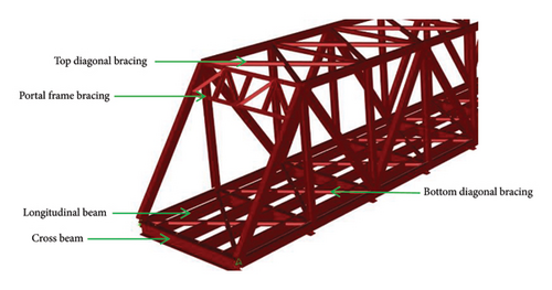
The bridge to be modeled for the study is a full-scale steel truss bridge with a concrete deck. It consists of diagonal members, bottom chord, top chord, bottom diagonal, top diagonal, cross beam, and longitudinal beams, as shown in Figure 2.

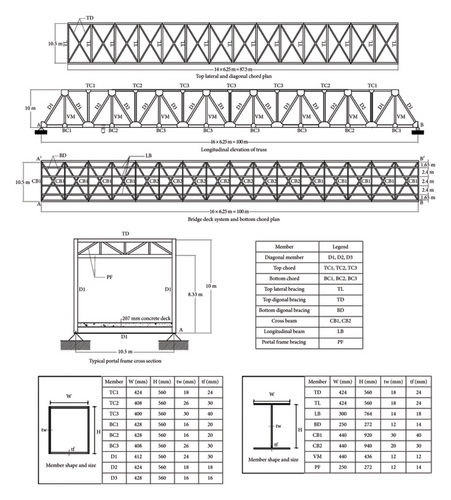
The bridge has two portal frames at the entry and exit. The members are made up of built-up sections with structural steel plates. The cross-section specification for each member is also illustrated in Figure 2. The diagonal members, top chords, and bottom chords are formed with hollow box sections. The vertical members, top diagonals, bottom diagonals, long beams, and portal frame bracings are formed using I-sections. The longitudinal beams support a concrete deck of 207 mm with an overlay of a 62-mm-thick mastic asphalt wearing course.

The steel grade of the truss members was ASTM A709 Grade 50 W. The concrete used in the deck has a compressive strength of 35 MPa. The entire bridge is designed to be simply supported by pin supports at one end and roller supports at the other. The individual bridge members were modeled to be pin-connected at their ends.

2.2. FEM

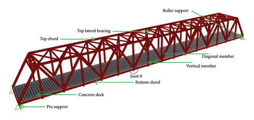
A multielement, stiffness-based FEM framework has been used to conduct a time-dependent structural response analysis under vehicle loading. FEM and analysis were performed using the commercially available software package CsiBridgev21 [56]. The steel and concrete used in the members and deck were modeled as isotropic materials following the specifications of the actual bridge. The steel truss bridge consists of steel members with a concrete deck overlay, as shown in Figure 3. The isotropic properties of steel and concrete used in the model are mentioned in Table 1. The bridge was modeled to be simply supported at its ends. It was restrained against translation in the UX, UY, and UZ directions at one end and against translation in the UY and UZ directions at the other. All the members were modeled to be pin connected at their i^th and j^th nodes.

Table 1. Isotropic properties of materials.

Material	Modulus of elasticity, E (MPa)	Unit mass, ρ (kg/m³)	Poisson’s ratio
Steel	200,000	7850	0.3
Concrete	24,860	2400	—

The deck was applied on top of the longitudinal beams as panels. The panels were divided into smaller meshes, each with an aspect ratio of 4:9. Each panel was divided into 36 small meshes. Smaller mesh sizes were also found to produce similar results. The cross beam and bottom chords were also divided into the same mesh size as the slab to ensure compatibility with the deck at the interface when it deflects under vehicle loading.

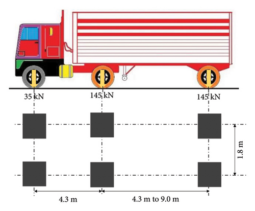
The dynamic load was applied using an HL-93 truck shown in Figure 4, which has been modeled to commute from one end of the bridge to the other in the positive X direction along a lane of 3.65 m width. The vehicle was modeled to enter the bridge at end A-A′ and exit at end B-B′, as indicated in Figure 2. The vehicle loading duration was 12 s with a speed of 10 m/s. In addition to the self-weight of the bridge, an external uniform load of 3.59 kN/m² was applied on the deck arising from the bitumen-wearing course.

2.3. Dynamic Analysis

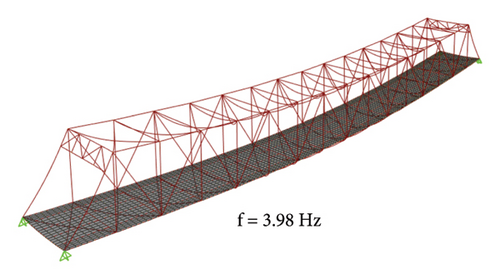
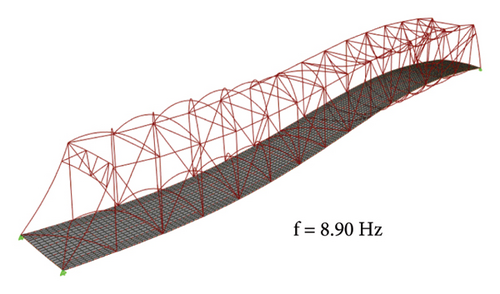
A direct integration approach using the Newmark’s Beta method was used to conduct the dynamic analysis, and a loading program was modeled accordingly. Newmark’s Beta method was used with a value of γ set as 0.5 and β set as 0.25. A Raleigh damping was utilized with a modal damping ratio of 0.4% as per reference [43]. The developed FEM of the bridge was then analyzed to obtain the response. The modal response of the bridge was obtained through eigenvalue analysis. The modes and modal frequencies for the first four vertical modes are typically presented in Figure 5. The modal responses depict that the range of frequencies for the first four vertical modes lies within the range for steel truss bridges obtained by earlier researchers [57]. However, the bridge would be classified as a stiff bridge having a high redundancy.

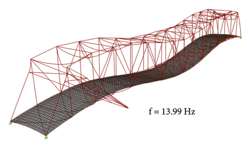
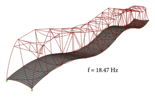
The acceleration response because of vehicle loading from dynamic time history analysis was sensed at a sampling frequency of 200 Hz. The response only corresponds to the forced vibration; that is, only the time from which the first axle of the vehicle enters the bridge to the instant when the last axle exits the bridge was considered in this study. The obtained acceleration response in the vertical direction is shown in Figure 6, typically for a Joint 8 (see Figure 3). The vertical acceleration response obtained from the model was similar to the study obtained in past research for steel truss bridges [43, 50].

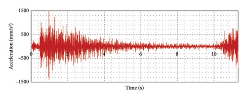
In Figure 6, the first three peaks correspond to when the three axles enter the bridge, eventually decreasing because of damping. At approximately 2 s, as the vehicle passes over the sensor location, the peak acceleration response increases again and decreases gradually because of bridge damping. The last set of peaks corresponds to when the vehicle exits the bridge.

3. Damage Detection Methodology

The study aims to detect damage from the acceleration response of the bridge from vehicle-induced vibration employing a semisupervised method using a deep learning technique and a statistical distance metric. This semisupervised learning scheme comprises BiLSTM and FCLs to train the network using sequence-to-sequence modeling based on the undamaged bridge state only. This section discusses the steps involved, from data preprocessing to the model architecture.

3.1. Semisupervised Learning Scheme Using BiLSTM

Our methodology generates input and output values from the same dataset. Moreover, the datasets are independent of labels. Sequence-to-sequence modeling has been adopted to serve this objective. This section elaborates on the adopted modeling approach. The acceleration response of the bridge in the healthy condition was used to prepare the dataset to train the network and then test the trained network. To simulate multiple test vehicle passes over the bridge and real-life situations where the measured response was contaminated by noise [44], 40 responses were generated, applying a 10% random noise each time to the response at Joint 8. Noise was incorporated into the response using Equation (1).

()

where X_m = acceleration response with noise; X = measure acceleration response; p = percentage of noise level; N_noise = gaussian noise distribution with standard normal distribution; and σ(X) = standard deviation of the measured acceleration response.

The noise-incorporated responses were then divided into 50 sets of data for training and validation and 20 sets of data for testing. Twenty percent of the data from the training dataset was used for validation. Each of the training, validation, and testing datasets was then standardized. As shown in Equation (2), the data were standardized to improve the training accuracy and speed [58].

()

where x_ij is the amplitude at the j^th time step of sample i of length L, x_mean is the mean of the sample i, σ is the standard deviation of the sample i, and X_{ij,standardized} is the standardized amplitude at the j^th time step of sample i.

3.1.1. Sequence Modeling of Vehicle-Induced Acceleration

The prepared datasets were arranged into sequences depending on the window size for sequence-to-sequence modeling. The window size dictates how many previous time steps should be used to predict a target value. Delay controls how many time steps to skip after the end of the window to get the target value. The target value is the value to be predicted in the dataset using the BiLSTM algorithm. A target value and the set of time steps within the window is considered a sample. Samples were generated with a sliding window with a step size of 1. The delay is set to zero. An overall description of arranging the dataset into sequence or sample is explained with an illustration in Figure 7.

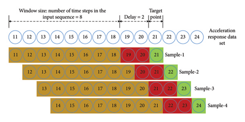
The training and test datasets consist of 112,500 and 45,000 sequences or samples, respectively. A validation set was also generated to control the model’s training. The 112,500 sequences of the training set were divided into 90,000 and 22,500 sequences. The BiLSTM model was then trained based on these prepared training and validation sets. The BiLSTM algorithm creates a mode that maps the input sequence to the target point.

3.2. Overview of LSTM Network

LSTM network overcomes the problems of exploding gradient and vanishing gradient problems faced by conventional RNNs. Using the cell state, it learns long-term dependencies among data in the time steps. At each time step, the LSTM unit learns data and removes data from the cell state. At each step, the LSTM cell also has a hidden state, which contains the output of the LSTM layer from that time step. Each LSTM cell comprises input gate i_t, forget gate f_t, cell candidate g_t and output gate o_t. All the gates, along with the cell state vector c and hidden state vector h, are shown in Figure 8.

The hidden state vector (h) and cell state vector (c) are of size p × 1, where p corresponds to the number of hidden states. In the figure, h_t−1 is the output vector of the previous state, and X_t is the current input. The LSTM cell passes h_t−1 and X_t through the sigmoid function to determine which information should be omitted from the existing cell state.

Each gate in the LSTM cell has learnable parameters. These are input weights W, recurrent weights R, and bias b. Each of the parameters for the four gates is concatenated into a matrix. The concatenated form is represented in Equations (3)–(5).

()

In the concatenated form, the subscripts i, f, g, and o denote the input gate, forget gate, cell candidate, and output gate, respectively. The operation executed in each of the gates at each time step is provided in Equations (6)–(9).

()

where σ_g is the sigmoid activation function and σ_c is the hyperbolic tangent activation function. The cell state at time step t is calculated by combining f_t, g_t, and i_t. The hidden state is calculated by combining the output gate and cell state. Equations (10) and (11) depict the computations.

()

where ⊙ denotes element-wise multiplication. The hidden state vector, h_t, cell state vector, c_t, and input data, X_t+1 are sent as input to the LSTM cell at the time step t + 1. In this manner, the hidden state vector and cell state vector output at time step t + 1 and data, X_t+2, at the time step t + 2 are used to calculate the hidden state vector and cell state vector input for t + 3. Subsequently, the hidden state output at the last time step is fed into a FCL to predict the target value for the data sequence of a sample.

3.3. Overview of Bidirectional LSTM (BiLSTM) Network

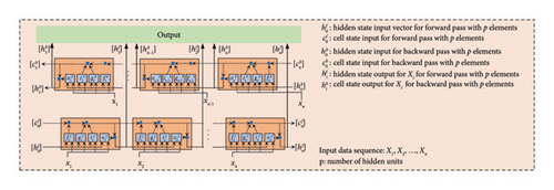
The BiLSTM network further transcends the LSTM network, incorporating a forward and backward pass. In the forward pass, each LSTM unit takes a hidden state vector, , cell state vector, , and a value from the data sequence, X_i, as input to give a hidden state vector, , and a cell state vector, , as output, as done for the LSTM network discussed in the earlier section.

The hidden states for the forward pass, h^f, and backward pass, h^b, and the cell states for the forward pass, c^f, and backward pass, c^b, are vectors of size p × 1, where p equals the number of hidden units. Consequently, the recurrent weight matrix, for a BiLSTM cell had a size of 8p × p. The operation of LSTM cells in the forward and backward pass is the same as the operation of an individual LSTM cell discussed in the earlier section.

A similar scheme is followed for the backward pass, but the data sequence is fed into the network, beginning with the last value in the sequence and continuing up to the first value of the sequence. The hidden state outputs from the forward pass, , and backward pass, , for the same time step are then concatenated to get the output from the BiLSTM Layer. This concatenated output, , is then used as input for the subsequent layer. A visual representation of how the BiLSTM network functions has been presented in Figure 9.

3.4. Model Architecture

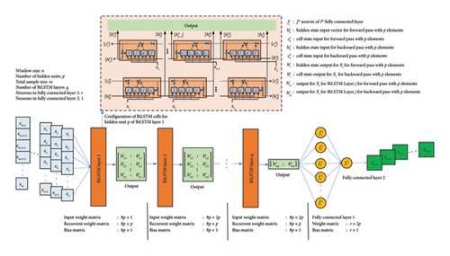
BiLSTM, a variant of RNN, is used in conjunction with FCLs to deal with the sequential data. A typical architecture comprising the input sequence, BiLSTM Layers, and FCL, used for the present study in bridge damage detection, is presented in Figure 10.

3.4.1. Network Optimization

To ensure an efficient and accurate network, the network needs to be optimized. Network optimization includes optimizing both the architecture and hyperparameters. The architecture optimization includes deciding the number of layers to be used. The layers include the BiLSTM layer, dropout layer, and FCLs. Mean squared error (MSE) was used as the loss function in training with the “Adam” optimizer. The final architecture was decided through trial based on the root MSE (RMSE) values of the test dataset. A range of BiLSTM layers ranging from 1 to 5 and FCLs ranging from 2 to 5 were experimented with. The effect of the number of neurons within the FCLs was also studied. The final architecture was then decided as four BiLSTM layers and two FCLs, with a dropout layer before and after the last BiLSTM layer to prevent overfitting. Once the training was complete, the model that had the least validation loss at the end of each epoch was selected as the trained model.

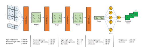
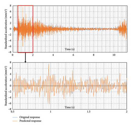
A thorough hyperparameter tuning analysis was conducted for the hyperparameter optimization based on the RMSE values of the test dataset. The range of values tested for different hyperparameters with their optimal configuration is presented in Table 2. The adopted network architecture to be used for damage detection in the bridge is presented in Table 3. An illustration of the architecture is also provided in Figure 11. The trained network with the selected hyperparameters is then applied to the test dataset. The trained model was found to fit the test data reasonably well, capturing all the peaks and troughs perfectly. The comparison between the predicted responses from the trained network by overlaying it over the actual response for a typical test dataset is presented in Figure 12, with an RMSE value of 0.0972. In the figure, the response within the first 3.5 s has been magnified to demonstrate the fit of the predicted response. The predicted response was a good fit with the actual response.

Table 2. Hyperparameters used for tuning the network.

Hyperparameter	Values	Optimal hyperparameters
Number of hidden units	8, 16, 32, 64, 128	64
Window size	8, 16, 32, 64, 128	16
Delay	0, 2, 5	0
Initial learning rate	0.008, 0.005, 0.003, 0.001, 0.0008	0.001
Learn rate drop period	50, 80, 90, 100	90
Learn rate drop factor	0.9, 0.8, 0.7, 0.5	0.9
Dropout layer probability	0.1, 0.2, 0.3, 0.4, 0.5	0.1
Max epoch	900, 1000, 1200, 1500, 2000, 2500	1500

Table 3. Final trained network architecture.

Layer	Hidden unit	Input size (sequence)	Output size (sequence)
Sequential input layer		1	—
BiLSTM Layer 1	64	1	128
BiLSTM Layer 2	64	128	128
BiLSTM Layer 3	64	128	128
Dropout layer		—	—
BiLSTM Layer 4	64	128	128
Dropout Layer		—	—
Fully connected Layer 1	16	128	16
Fully connected Layer 2	1	16	1

3.5. Damage-Sensitive Feature Generation and Discrimination

The trained network is referred to as the baseline model. The damage detection scheme comprises two major steps: damage-sensitive feature extraction and feature discrimination [21].

The prediction error is considered as the damage-sensitive feature, and KLD is used as the statistical metric for feature discrimination. The training data sequences are passed through the baseline model, and the prediction error vector, referred to as the reference error vector, e_r is calculated. The 20 reference error vectors are determined for the 20 training datasets. Further, test error vectors, e_b, are calculated similarly to the test datasets.

It is observed that the errors between the predicted and original responses followed a normal distribution. Therefore, a statistical distance metric called the KLD has been used as a metric to discriminate between the original response and the predicted response. It will give us a measure of the difference between errors of the predicted and actual responses for feature discrimination to detect damage.

The KLD, which is also referred to as relative entropy or I-divergence [59], is a univariate distance approach proposed by Kullback and Leibler in 1951. KLD is a nonsymmetric measure of the difference between two probability distributions or probability density functions (PDF). It is denoted by d_kld(P_x‖P_z), which is a statistical measure of how one PDF P_x is different from a second reference PDF P_z. It is expressed mathematically according to Equation (12).

()

The KLD value lies between 0 and greater values. A value that deviates from 0 is indicative of dissimilarity between two distributions. KLD is appropriate for random high-dimensional data samples [60]. If P_x and P_z are two PDFs that have a normal distribution, then Equation (12) can be further simplified into Equation (13) [61], where μ₁, σ₁ and μ₂, σ₂ are the mean and standard deviation of P_x and P_z, respectively.

()

If e_u and e_d represent the vector for the residual between the actual response and predicted response for the undamaged and damaged states, respectively, we can calculate the μ and σ for each of the vectors. Comparing them using Equation (13), we can ascertain by how much the PDF of e_d differs from e_u.

The unknown state acceleration responses of the bridge are then preprocessed, as discussed in Section 3.1. The responses are arranged into sequences and passed through the baseline model, and the prediction error vector, denoted as e_d, is calculated for this state. Subsequently, the distance between e_r and e_b is calculated using the distance metric KLD, which is referred to as baseline . Similarly, the distance between e_r and e_d is calculated for the unknown states using the distance metric, KLD, which is referred to as the unknown state . The step-by-step process to calculate the is presented in Figure 13.

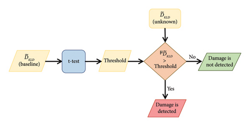
Then, a one-tailed t-test is conducted on the baseline at 95% confidence level to get a threshold against which the damaged case values will be compared. The mean and standard deviation for e_b, e_r,, and e_d are calculated using the mean likelihood estimate (MLE). A larger value of the mean of the unknown state , denoted as , will confirm the presence of damage. A flowchart of the process involved in confirming the presence of damage is presented in Figure 14.

4. Damage Scenario

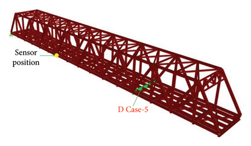
To evaluate the performance of the proposed methodology in detecting damage in a bridge, an acceleration response is collected from the bridge after simulating damage in the FEM of the bridge. The damage to bridges in the form of corrosion and rust results in a reduction of the stiffness of different members in the bridge [62, 63]. The damage is induced by stiffness reduction through a reduction in the elastic modulus [64] in the bottom chords and top chords of both the truss webs of the bridge as well as the cross beams and a diagonal member. The members into which the damage is introduced for the present study are shown in Figure 15. Four different levels of damage are considered.

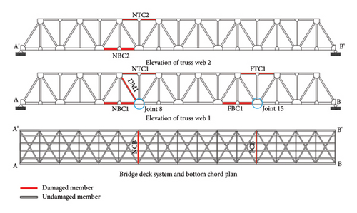
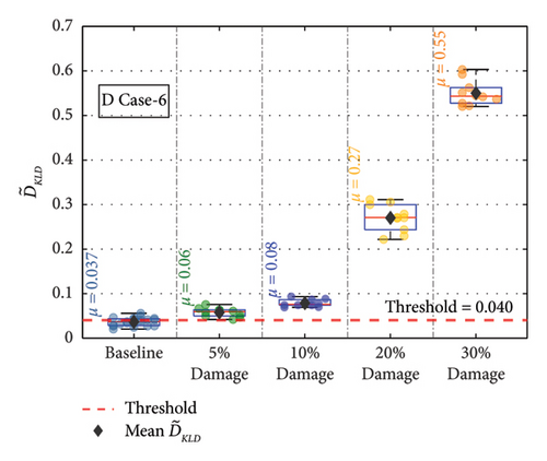
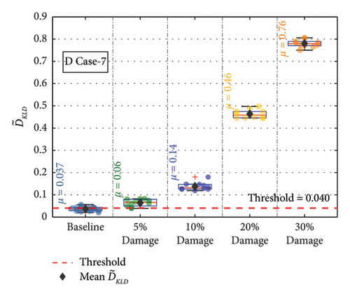
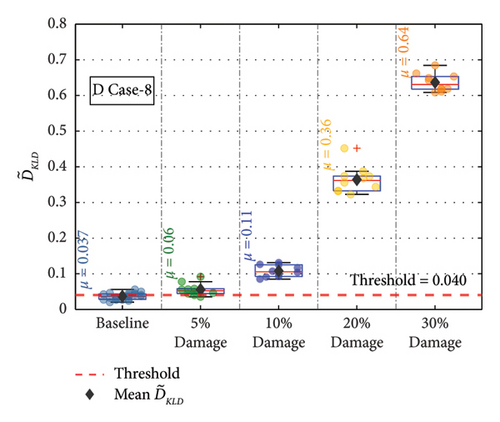
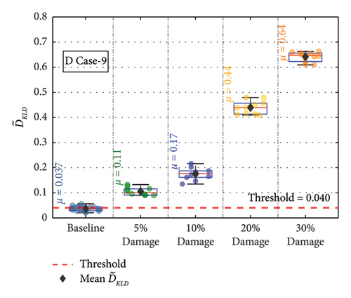
The description of the nomenclature of each of the members into which the damage is introduced is given in Table 4. The members were classified as far and bottom depending on the relative distance from Joint 8. A damaged case number was assigned to each of the damage scenarios. Three damage scenarios simulated in the FEM are typically shown in Figure 16. Eight different damage cases are considered, with four different damage levels per member. Thus, a total of 36 different damage scenarios are considered individually for a single sensor position in evaluating the efficacy of the proposed method in detecting damage in the bridge using vehicle-induced vibration.

Table 4. Damaged member description.

Damage case	Member name	Member description	Truss web	Damage level (%)
D Case 1	NBC1	Near bottom chord	1	5, 10, 20, 30
D Case 2	FBC1	Far bottom chord	1	5, 10, 20, 30
D Case 3	NBC2	Near bottom chord	2	5, 10, 20, 30
D Case 4	NCB	Near cross beam	—	5, 10, 20, 30
D Case 5	FCB	Far cross beam	—	5, 10, 20, 30
D Case 6	NTC1	Near top chord	1	5, 10, 20, 30
D Case 7	FTC1	Far top chord	1	5, 10, 20, 30
D Case 8	NTC2	Near top chord	2	5, 10, 20, 30
D Case 9	DM1	Diagonal member	1	5, 10, 20, 30

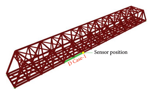
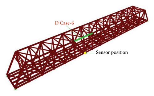
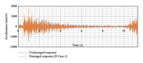
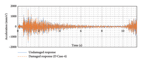
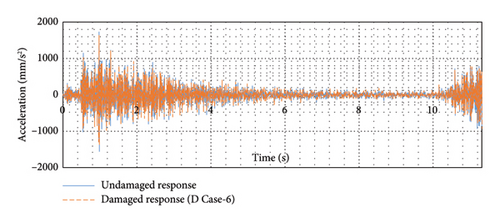
The acceleration response from Joint 8 in the damaged condition for different damage scenarios was obtained by passing a test vehicle over the damaged bridge, as was done for the undamaged bridge. The difference in response between the damaged and undamaged conditions cannot be discerned visually, as seen in Figure 17, for the different damage cases.

5. Damage Detection Result

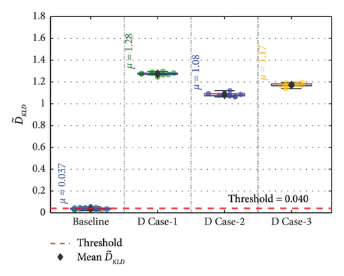
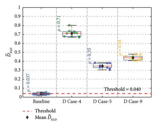
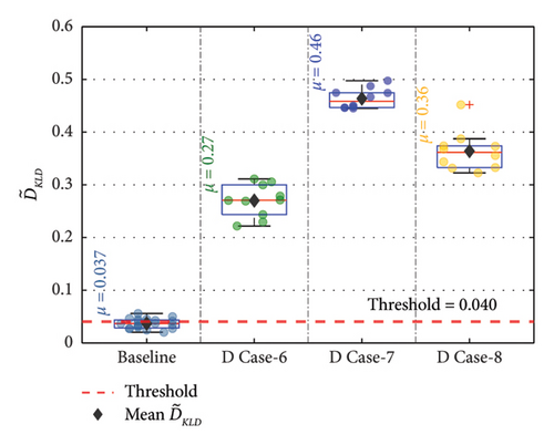
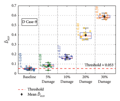
Nine members were evaluated to detect the presence of damage in the bridge using the adopted methodology. The for the three bottom chords, two cross beams, three top chords, and one diagonal member against the threshold value at 20% damage severity level are presented in Figures 18(a), 18(b), and 18(c). The values, along with for each of the damaged cases, are plotted with distinct colors within the region bounded by vertical lines. In all the damaged cases, the is greater than the threshold value. This confirms that the proposed methodology can detect damages in the bridge. Moreover, it can be observed from Figure 18 that the deviation of from the threshold is more prominent for the bottom chords than the cross beams, top chords, and diagonal member.

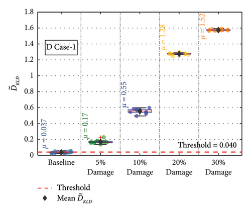
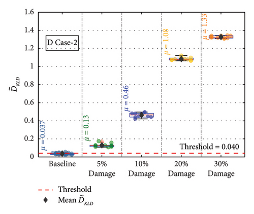
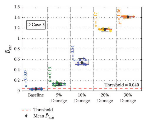
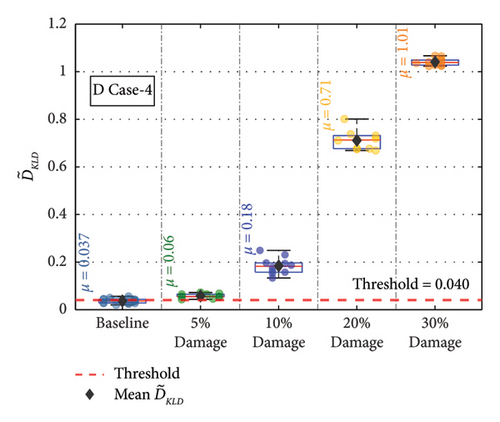
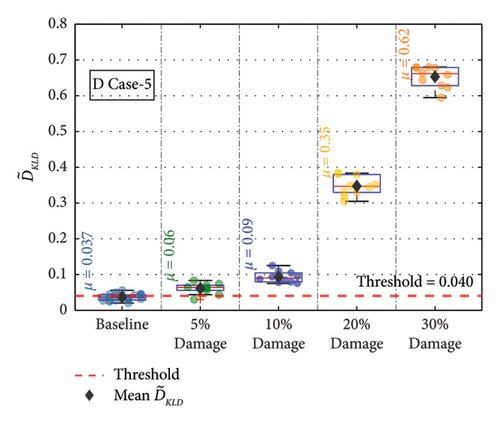
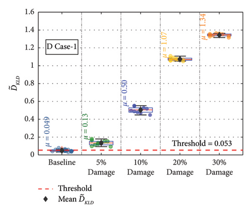
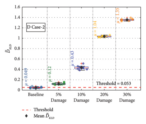
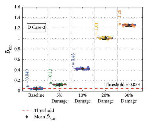
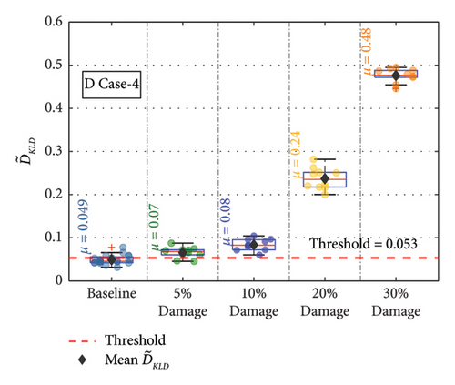
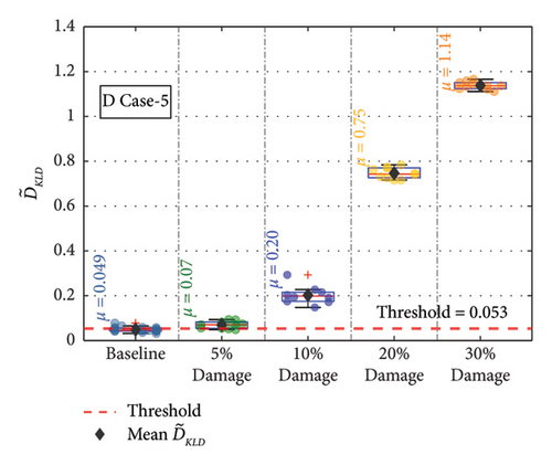
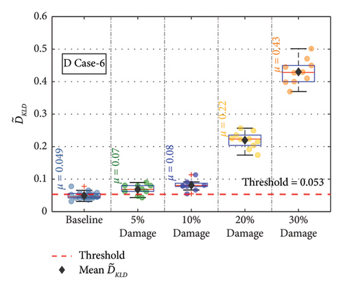
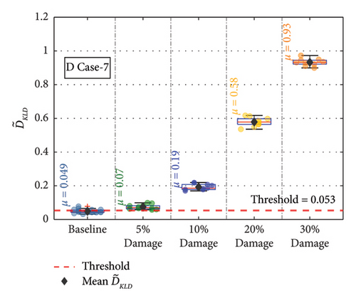
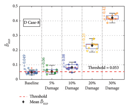
For the remaining damage levels, the efficacy of the methodology has been investigated similarly. The damage index , against the threshold value for nine damaged cases with four different damage levels, is presented separately in Figures 19(a), 19(b), 19(c), 19(d), 19(e), 19(f), 19(g), 19(h), and 19(i), respectively. The figures reveal that is higher than the threshold set by the t-test for all the cases. This confirms the capability of the proposed technique to discriminate the various damage scenarios in the bridge. Moreover, the methodology is also successful in identifying gradual damage. The value increases with the damage severity level in all the damaged cases.

5.1. Effect of Sensor Position

The acceleration responses from Joint 15, shown in Figure 15, were used to evaluate the effect of sensor position in damage detection. The damaged members and damaged cases remained unchanged. Data preprocessing methodology and network architecture were maintained similarly to that for Joint 8. The network was trained using the newly prepared datasets, and the hyperparameters were optimized based on the test dataset’s RMSE values. The hyperparameter values used for this network are mentioned in Table 5.

Table 5. Optimal hyperparameter value.

Hyperparameter	Value
Number of hidden units	64
Window size	16
Mini batch size	9436
Delay	0
Initial learning rate	0.001
Learn rate drop period	90
Learn rate drop factor	0.9
Dropout layer probability	0.1
Max epoch	1500

The for the members at different damage conditions were calculated and compared against the threshold value. The at the different damage levels for the various members are shown separately in Figures 20(a), 20(b), 20(c), 20(d), 20(e), 20(f), 20(g), 20(h), and 20(i). In Figure 20, the values at each damage level along with are plotted for the different damage severity levels. The methodology is successful in detecting all the damage scenarios. The value increases with the damage severity level in all the damaged cases. This confirms the capability of the methodology in detecting damages irrespective of the sensor location in the bridge.

5.2. Damage Detection for Damage in Multiple Members

The methodology’s performance for multiple damaged members in the bridge was evaluated. To evaluate its performance, a new damage scenario named D Case-10 was introduced. In D Case-10, damages were induced simultaneously in the bottom chord close to Joint8 (NBC1) and top chord away from the Joint 8 (FTC1), as indicated in Figure 15. Two levels of damage at 5% and 10% were considered for this study. The performance of the methodology for D Case-10 was then compared against the individual damage cases of such members, namely, D Case-1 and D Case-7, as shown in Figures 21(a) and 21(b).

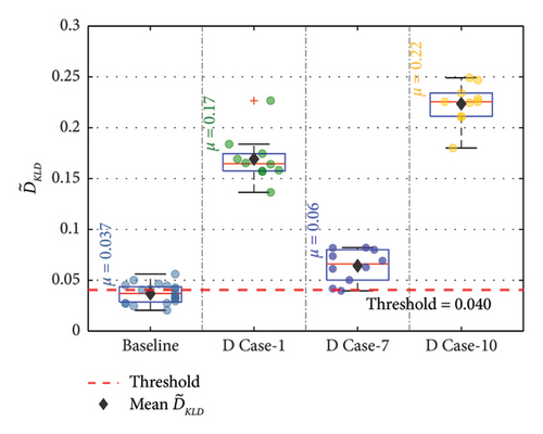
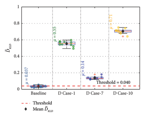
Figure 21 shows that when multiple members are damaged, the deviation of from the threshold increases than that of individual damage cases for the same damage severity. At both the damage severity levels, the deviation from the threshold is greater for the multiple damaged state than the individual damage state. This confirms the capability of the methodology in detecting damage when multiple members are damaged at the same time.

5.3. Performance Under Operational Variations

In order to evaluate the practical applicability of the methodology, its performance needs to be evaluated under operational variations. The operational variation was introduced in the FE model by varying the test vehicles in the undamaged state of the bridge.

To prepare the training dataset, five different test vehicles were considered by varying the axle loads of each vehicle as a percentage of the axle loads of the HL-93 test vehicle. The five different vehicles used to prepare the training and testing datasets are shown in Table 6. Fifty datasets for training and 20 datasets for testing were then prepared for each test vehicle by incorporating a 10% random noise into the acceleration response obtained from Joint 8.

Table 6. Test vehicles for operational variation.

Test vehicle no.	Axle weight as % of HL-93 (%)
1	50
2	90
3	100
4	110
5	150

Once the datasets were prepared, the final network architecture was established and hyperparameters were optimized. The network architecture was found to be the same as in Figure 11 with an alteration of the removal of dropout layers and addition of a single BiLSTM layer. The optimized hyperparameters are shown in Table 7.

Table 7. Optimal hyperparameters for evaluation of vehicle operation.

Hyperparameter	Value
Number of hidden units	64
Window size	32
Mini batch size	11,250
Delay	0
Initial learning rate	0.001
Learn rate drop period	90
Learn rate drop factor	0.9
Dropout layer probability	0.1
Max epoch	1500

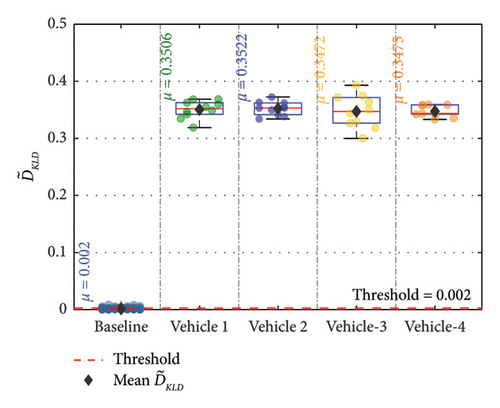
A one-tailed t-test at 95% confidence level was then conducted to calculate a threshold for the test vehicles. Next, four unknown vehicles different from those used in training were run over the undamaged bridge. Upon evaluating the responses by the baseline model, the method should identify the state as undamaged. The four vehicles used to prepare the unknown state response of the bridge are shown in Table 8. Two vehicles were kept within the range of the vehicles used for training the dataset, while the other two vehicles were kept outside the range. A 10% random noise was then introduced into each acceleration response from Joint 8 to prepare 10 datasets for evaluation. A comparison of the mean for the undamaged state for the four unknown vehicles has been shown in Figure 22.

Table 8. Unknown vehicles for evaluation of operational variation.

Unknown vehicle no.	Axle weight as % of HL-93 (%)
Vehicle 1	80
Vehicle 2	120
Vehicle 3	40
Vehicle 4	160

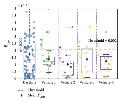
From Figure 22, it is observed that, for an unknown vehicle, the mean value is less than the threshold for the baseline state of the bridge. The methodology thus confirms the state as a undamaged condition of the bridge. If the methodology was not successful, it would have considered the response from an unknown vehicle as a damaged state with a mean value greater than the threshold. The methodology was then evaluated in detecting damage for D Case-1 at a 10% damage level because of operational variation for the four vehicles mentioned in Table 8. The performance of the methodology in detecting damage is demonstrated in Figure 23. The methodology was successful in detecting damage for D Case-1 at a 10% damage level for all four vehicles. This confirms the potential of the methodology to be used under varying vehicles.

6. Experimental Validation on Old ADA Steel Bridge Measurements

The proposed methodology in the earlier section was then evaluated to detect damage using full-scale vibrational measurements from an actual bridge experiment with vehicle-induced vibration to validate its real-world applications. The vibrational measurements from the benchmark data, such as the Old ADA Steel Truss Bridge, were used.

6.1. Bridge and Loading Vehicle

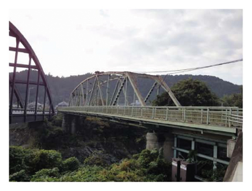
The steel truss bridge is located in the Nara Prefecture of Japan. The bridge is simply supported and spans 59.2 m, having a width of 3.6 m and a maximum height of 8.2 m. A series of tests were conducted on the bridge before its replacement in 2012. When performing the tests, traffic movement was stopped to ensure safety and avoid interruption. A picture of the bridge is given in Figure 24.

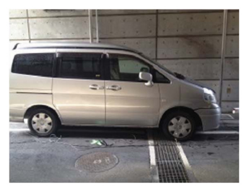
For information related to the experiment, equipment, and test scenario, Chang and Kim [21] can be consulted. The bridge was excited using a two-axle reaction vehicle (Serena Model: Nissan Motor Co. Ltd). The vehicle had a total weight of 21 kN, including the passenger and measurement devices. The frequencies associated with sprung motion at the front and rear axle of the vehicle were identified to be 1.7–1.8 Hz and 2.1–2.3 Hz, respectively. The figure of the test vehicle is presented in Figure 25.

6.2. Sensor Placement and Test Scheme

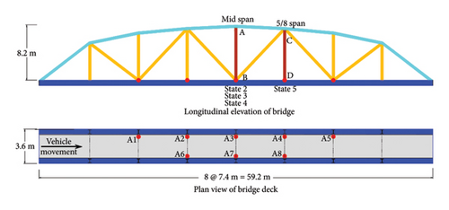
Because of vehicle-induced vibration, the acceleration response of the bridge in the vertical direction was collected using uniaxial accelerometers placed at eight different nodes along the bridge. The accelerometers had a sampling frequency of 200 Hz. Five sensors (A1–A5) were placed on one truss web, while the remaining three sensors (A6–A8) were placed on the opposite truss web. Two optical sensors were also placed at the entry and exit points of the bridge to monitor the vehicle entrance and exit. The location of the sensors on the bridge is provided in Figure 26.

6.3. Test Scenarios

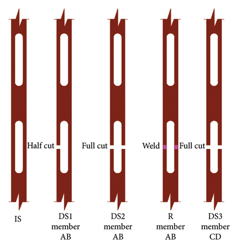
The bridge was tested under vehicle-induced vibration in five realistic states, from State 1 to State 5. The states were created by inducing damage and repair of the bridge members “AB” and “CD” in Figure 23. The baseline case in the undamaged state was assigned to State 1. Acceleration readings were obtained from all eight sensors at varying speeds of the test vehicle. However, the present study has used acceleration readings at 40 km/h. Details of the damage scenario have been summarized in Table 9. However, it should be noted that, at State 4, the complete restoration of the bridge to its original state was not guaranteed [21]. The five different damage scenarios in the members of the bridge have been shown in Figure 27.

Table 9. Damage scenarios in Old ADA Bridge.

State	Label	Condition	Damage scenario	Number of repetitions
State 1	IS	Undamaged	Intact condition	10
State 2	DS1	Damaged	Cut halfway along the depth of member AB	12
State 3	DS2	Damaged	Full cut along the depth of member AB	10
State 4	R	Recovered	Welding along the full cut of member AB	10
State 5	DS3	Damaged	Full cut along the depth of member AB	10

6.4. Data Preprocessing

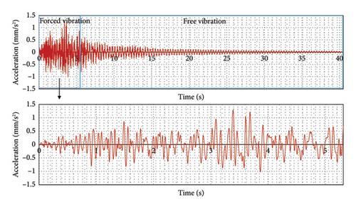
In the damage detection scheme, State 1 was used as a baseline state in the damage detection for State 2 and State 3. State 4 was used as a baseline case in the damage detection for State 5. The data obtained in the repository [54] contain the free and forced vibration response. The response corresponding only to the forced vibration part has been used to train the DL model. Each state’s sensor response had multiple passes of the vehicle. The forced acceleration response was then standardized for each pass. The step-by-step process involved in data extraction is illustrated in Figure 28.

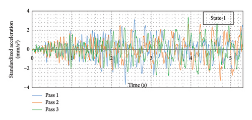
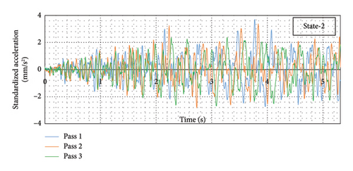
A comparison of standardized forced acceleration response for three different passes has been presented in Figure 29. The figure shows that the recorded acceleration responses for different passes of the test vehicle are not entirely identical. Such variation is expected and can be attributed to the coupled dynamic system for vehicle bridge interaction and road roughness. Detecting damage despite these variations in recorded data will establish the robustness and reliability of the methodology in bridge damage detection.

6.5. Network Optimization

Standardized data were then arranged into sequences to train the numerical model discussed in the previous section. The first five datasets were used in training from the baseline data, while the remaining five were used as the test dataset. From the training dataset, 20% of the prepared data sequences were used as the validation set. A model was then trained using the training dataset.

Sequences of the standardized data for State 1 (baseline state) were then used to train a BiLSTM model architecture, which would be used in bridge damage detection. The network architecture and hyperparameters, which gave the minimum RMSE value for the actual response and predicted response for sensor A1, are provided in Table 10. Two BiLSTM layers were used with two dropout layers before and after the last BiLSTM Layer. Two FCLs were also used after the BiLSTM layers, as done for the FEM. Before creating damaged State 5 of the bridge, recovery was done by welding the damaged member AB. The recovered State 4 was considered as the baseline state for the damaged State 5.

Table 10. Optimal hyperparameter values for State 1 and State 4.

Hyperparameter	Value (State 1)	Value (State 4)
Number of hidden units	8	32
Window size	16	16
Mini batch size	4128	4216
Delay	0	0
Initial learning rate	0.005	0.005
Learn rate drop period	100	100
Learn rate drop factor	0.9	0.9
Dropout layer probability	0.2	0.2
Max epoch	2500	2500

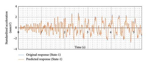
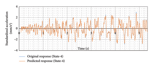
An overlay shows the predicted response over the actual response for sensor A1 in Figure 30 for both states. The figure indicates that the trained model could predict the response quite well because of vehicle-induced vibration for both states. The trained model was then used to predict the presence of damage in the bridge using the same methodology applied to the FEM.

6.6. Damage Detection Results

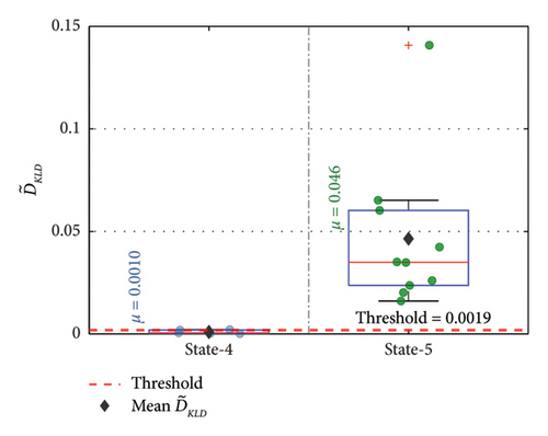
Two members were evaluated to detect the presence of damage in the bridge using the adopted methodology. For State 2 and State 3, State 1 was used as the baseline condition, and for State 5, State 4 was used as the baseline condition. The for State 2 and State 3 against the threshold value is presented in Figure 31.

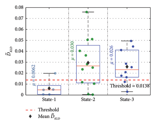
In the figure, the adopted methodology can detect the presence of damage for both the states using a single sensor response, as the value is well above the threshold value for both the states. The for State 5 against the threshold value is presented in Figure 32. In the figure, the mean is greater than the threshold value for the damaged condition response at State 5. Thus, the proposed methodology can detect damage states using a single sensor response in a real-world field experimental bridge. Even though the sensor position A1 is chosen far from the damaged location, the proposed method successfully detects all the damaged states in the bridge.

7. Conclusions

Conventional BHM methods are a rather time-consuming, expensive, and erroneous process. The inception of ML algorithms and their transcendence into data science has opened a gateway to applying these tools to BHM. However, the scarcity of damaged bridge data, a requisite for training ML models, hinders its application to BHM. The present study aims to circumvent this hindrance and investigate the efficacy of a novel methodology comprising a semisupervised BiLSTM architecture for feature extraction and KLD for feature discrimination. The method is first numerically investigated on damage detection of an FE model of a real steel truss bridge using sequence-to-sequence modeling of vehicle-induced acceleration response.

The BiLSTM network model is then trained using the sequences developed from the acceleration response from a single sensor position. Hyperparameters of the model are optimized using the training and validation set of sequences. Damage is then induced into the structural members of the bridge by stiffness reduction. The discrimination between the bridge’s damaged and undamaged state is performed using a proposed damage index,

. The efficacy of the methodology under multiple damage scenarios and vehicle operation variations has also been evaluated. The proposed methodology has then been applied for detecting damage in a bridge in a real-world scenario. The acceleration response of a single sensor from the “Old ADA Bridge” test under varying damaged conditions has been used to validate the applicability of the methodology. The following specific conclusions have then been drawn from the study:

i.
The developed semisupervised BiLSTM modeling approach supplemented by damage index, , successfully detects not only all the damage scenarios considered but also gradual damage in all damaged cases studied.
ii.
The sensor position does not affect the method’s efficacy in detecting bridge damage. However, the hyperparameters need to be optimized, keeping the architecture intact with the change in sensor location for bridge damage detection.
iii.
The proposed semisupervised methodology requires only data from the undamaged state of the bridge without the need for any labeled data from the damaged state, and it does not require any artificial excitation.
iv.
The proposed methodology is validated and proved to be effective in detecting damage in a bridge in a real-world scenario using only a single sensor response.
v.
The proposed methodology is capable of functioning under varying vehicular operation.

It is important to note that the experimental study used for the validation of the method was conducted in a controlled environment, which may influence the method’s performance under environmental and operational variations. This is because of the lack of experimental data comprising varying vehicles passing the bridges in undamaged and damaged states and with changing environmental conditions. Further studies have to be explored accounting for these factors to prove the robustness of the method for practical applications.

Conflicts of Interest

The authors declare no conflicts of interest.

Funding

No funding was received for this research.

Acknowledgments

The authors would like to thank Professor Chul-Woo Kim, Department of Civil and Earth Resources Engineering, Kyoto University, Kyoto, Japan, for sharing the data of the steel truss bridge utilized in this research work.

Open Research

Data Availability Statement

The proposed methodology is validated on a real field vibration measurement performed on the Old ADA Steel Truss Bridge located in Japan. The measurements were collected, published, and uploaded by Kim et al. [21, 53]. References have been cited in this article. The data of the Old ADA Bridge are available online at https://doi.org/10.17632/sc8whx4pvm.2

References

1 Eurocode 1: Basics of Structural Design, 2002, British Standards Institution.
Google Scholar
2 AASTHO Officials, Bridging the Gap-Restoring and Rebuilding the Nation’s Bridges, 2008, American Association of State Highway and Transportation Officials.
Google Scholar
3 Lopez R. and Love P. E. D., Design Error Costs in Construction Projects, Journal of Construction Engineering and Management. (2012) 138, no. 5, 585–593, https://doi.org/10.1061/(ASCE)CO.1943-7862.0000454, 2-s2.0-84862065021.
10.1061/(ASCE)CO.1943-7862.0000454
Web of Science® Google Scholar
4 He Z., Li W., Salehi H., Zhang H., Zhou H., and Jiao P., Integrated Structural Health Monitoring in Bridge Engineering, Automation in Construction. (2022) 136, https://doi.org/10.1016/j.autcon.2022.104168.
10.1016/j.autcon.2022.104168
Web of Science® Google Scholar
5 González A., Obrien E. J., and McGetrick P. J., Identification of Damping in a Bridge Using a Moving Instrumented Vehicle, Journal of Sound and Vibration. (2012) 331, no. 18, 4115–4131, https://doi.org/10.1016/j.jsv.2012.04.019, 2-s2.0-84861636398.
10.1016/j.jsv.2012.04.019
Web of Science® Google Scholar
6 Das S. and Saha P., A Review of Some Advanced Sensors Used for Health Diagnosis of Civil Engineering Structures, Measurement. (2018) 129, 68–90, https://doi.org/10.1016/j.measurement.2018.07.008, 2-s2.0-85049556615.
10.1016/j.measurement.2018.07.008
Web of Science® Google Scholar
7 Rodrigues C., Cavadas F., Félix C., and Figueiras J., FBG Based Strain Monitoring in the Rehabilitation of a Centenary Metallic Bridge, Engineering Structures. (2012) 44, 281–290, https://doi.org/10.1016/j.engstruct.2012.05.040, 2-s2.0-84863821098.
10.1016/j.engstruct.2012.05.040
Web of Science® Google Scholar
8 Bakht B. and Aftab M., BRIDGES: Analysis, Design, Structural Health Monitoring, and Rehabilitation, 2018, Springer International Pu.
Google Scholar
9 Almasri N., Sadhu A., and Ray Chaudhuri S., Toward Compressed Sensing of Structural Monitoring Data Using Discrete Cosine Transform, Journal of Computing in Civil Engineering. (2020) 34, no. 1, https://doi.org/10.1061/(ASCE)CP.1943-5487.0000855.
10.1061/(ASCE)CP.1943-5487.0000855
Web of Science® Google Scholar
10 Gatti M., Structural Health Monitoring of an Operational Bridge: A Case Study, Engineering Structures. (2019) 195, 200–209, https://doi.org/10.1016/j.engstruct.2019.05.102, 2-s2.0-85066863453.
10.1016/j.engstruct.2019.05.102
Web of Science® Google Scholar
11 Singh P. and Sadhu A., Limited Sensor-Based Bridge Condition Assessment Using Vehicle-Induced Nonstationary Measurements, Structures. (2021) 32, 1207–1220, https://doi.org/10.1016/j.istruc.2021.03.091.
10.1016/j.istruc.2021.03.091
Web of Science® Google Scholar
12 Carden E. P. and Fanning P., Vibration Based Condition Monitoring: A Review, Structural Health Monitoring. (2004) 3, no. 4, 355–377, https://doi.org/10.1177/1475921704047500, 2-s2.0-33644795626.
10.1177/1475921704047500
Web of Science® Google Scholar
13 Fan W. and Qiao P., Vibration-Based Damage Identification Methods: A Review and Comparative Study, Structural Health Monitoring. (2011) 10, no. 1, 83–111, https://doi.org/10.1177/1475921710365419, 2-s2.0-79751492551.
10.1177/1475921710365419
Web of Science® Google Scholar
14 Ritto T. G. and Rochinha F. A., Digital Twin, Physics-Based Model, and Machine Learning Applied to Damage Detection in Structures, Mechanical Systems and Signal Processing. (2021) 155, https://doi.org/10.1016/j.ymssp.2021.107614.
10.1016/j.ymssp.2021.107614
Web of Science® Google Scholar
15 Alves V. N., De Oliveira M. M., Ribeiro D., Calçada R., and Cury A., Model-Based Damage Identification of Railway Bridges Using Genetic Algorithms, Engineering Failure Analysis. (2020) 118, https://doi.org/10.1016/j.engfailanal.2020.104845.
10.1016/j.engfailanal.2020.104845
Web of Science® Google Scholar
16 Liu T., Zhang Q., Zordan T., and Briseghella B., Finite Element Model Updating of Canonica Bridge Using Experimental Modal Data and Genetic Algorithm, Structural Engineering International. (2016) 26, no. 1, 27–36, https://doi.org/10.2749/101686616X14480232444405, 2-s2.0-84984666946.
10.2749/101686616X14480232444405
Web of Science® Google Scholar
17 Tran-Ngoc H., Khatir S., De Roeck G., Bui-Tien T., Nguyen-Ngoc L., and Abdel Wahab M., Model Updating for Nam O Bridge Using Particle Swarm Optimization Algorithm and Genetic Algorithm, Sensors. (2018) 18, no. 12, https://doi.org/10.3390/s18124131, 2-s2.0-85057534018.
10.3390/s18124131
Web of Science® Google Scholar
18 Saadatmorad M., Talookolaei R.-A. J., Pashaei M.-H., Khatir S., and Wahab M. A., Pearson Correlation and Discrete Wavelet Transform for Crack Identification in Steel Beams, Mathematics. (2022) 10, no. 15, https://doi.org/10.3390/math10152689.
10.3390/math10152689
Web of Science® Google Scholar
19 Simoen E., De Roeck G., and Lombaert G., Dealing with Uncertainty in Model Updating for Damage Assessment: A Review, Mechanical Systems and Signal Processing. (2015) 56–57, 123–149, https://doi.org/10.1016/j.ymssp.2014.11.001, 2-s2.0-84919705008.
10.1016/j.ymssp.2014.11.001
Web of Science® Google Scholar
20 Santos J. P., Orcesi A. D., Crémona C., and Silveira P., Baseline-Free Real-Time Assessment of Structural Changes, Structure and Infrastructure Engineering. (2015) 11, no. 2, 145–161, https://doi.org/10.1080/15732479.2013.858169, 2-s2.0-84908481276.
10.1080/15732479.2013.858169
Web of Science® Google Scholar
21 Kim C.-W. and Chang K.-C., Modal-Parameter Identification and Vibration-Based Damage Detection of a Damaged Steel Truss Bridge, Engineering Structures. (2016) 122, 156–173, https://doi.org/10.1016/j.engstruct.2016.04.057, 2-s2.0-84977134499.
10.1016/j.engstruct.2016.04.057
Web of Science® Google Scholar
22 Xu D., Xu X., Forde M. C., and Caballero A., Concrete and Steel Bridge Structural Health Monitoring—Insight into Choices for Machine Learning Applications, Construction and Building Materials. (2023) 402, https://doi.org/10.1016/j.conbuildmat.2023.132596.
10.1016/j.conbuildmat.2023.132596
Web of Science® Google Scholar
23 Sun H., Song L., and Yu Z., A Deep Learning-Based Bridge Damage Detection and Localization Method, Mechanical Systems and Signal Processing. (2023) 193, https://doi.org/10.1016/j.ymssp.2023.110277.
10.1016/j.ymssp.2023.110277
Web of Science® Google Scholar
24 Salehi H. and Burgueño R., Emerging Artificial Intelligence Methods in Structural Engineering, Engineering Structures. (2018) 171, 170–189, https://doi.org/10.1016/j.engstruct.2018.05.084, 2-s2.0-85047606626.
10.1016/j.engstruct.2018.05.084
Web of Science® Google Scholar
25 Sun L., Shang Z., Xia Y., Bhowmick S., and Nagarajaiah S., Review of Bridge Structural Health Monitoring Aided by Big Data and Artificial Intelligence: From Condition Assessment to Damage Detection, Journal of Structural Engineering. (2020) 146, no. 5, https://doi.org/10.1061/(ASCE)ST.1943-541X.0002535.
10.1061/(ASCE)ST.1943-541X.0002535
Web of Science® Google Scholar
26 Mousavi M. and Gandomi A. H., Structural Health Monitoring Under Environmental and Operational Variations Using MCD Prediction Error, Journal of Sound and Vibration. (2021) 512, https://doi.org/10.1016/j.jsv.2021.116370.
10.1016/j.jsv.2021.116370
Web of Science® Google Scholar
27 Bishop C. M., Neural Networks for Pattern Recognition, 1995, Clarendon Press; Oxford University Press.
10.1093/oso/9780198538493.001.0001
Google Scholar
28 Rumelhart D. E., Hinton G. E., and Williams R. J., J. A. Anderson and E. Rosenfeld, Learning Internal Representations by Error Propagation, Parallel Distributed Processing: Explorations in the Microstructure of Cognition, 1988, Foundations, The MIT Press, Cambridge, MA, 675–695, https://doi.org/10.7551/mitpress/4943.003.0128.
Google Scholar
29 Nguyen D. H., Tran-Ngoc H., Bui-Tien T., De Roeck G., and Wahab M. A., Damage Detection in Truss Bridges Using Transmissibility and Machine Learning Algorithm: Application to Nam O Bridge, Smart Structures and Systems. (2020) 26, 35–47, https://doi.org/10.12989/SSS.2020.26.1.035.
10.12989/SSS.2020.26.1.035
Web of Science® Google Scholar
30 Zhao D., Ren Y., Huang Q., and Xu X., Analysis of Temperature-Induced Deflection of Cable-Stayed Bridge Based on BP Neural Network, IOP Conference Series: Earth and Environmental Science. (2019) 242, https://doi.org/10.1088/1755-1315/242/6/062075, 2-s2.0-85064390097.
10.1088/1755-1315/242/6/062075
Google Scholar
31 Nguyen-Ngoc L., Nguyen-Huu Q., De Roeck G., Bui-Tien T., and Abdel-Wahab M., Deep Neural Network and Evolved Optimization Algorithm for Damage Assessment in a Truss Bridge, Mathematics. (2024) 12, no. 15, https://doi.org/10.3390/math12152300.
10.3390/math12152300
Web of Science® Google Scholar
32 Khodabandehlou H., Pekcan G., and Fadali M. S., Vibration-Based Structural Condition Assessment Using Convolution Neural Networks, Structural Control and Health Monitoring. (2018) https://doi.org/10.1002/stc.2308, 2-s2.0-85058398443.
10.1002/stc.2308
Google Scholar
33 Alipour M., Harris D. K., and Miller G. R., Robust Pixel-Level Crack Detection Using Deep Fully Convolutional Neural Networks, Journal of Computing in Civil Engineering. (2019) 33, no. 6, https://doi.org/10.1061/(ASCE)CP.1943-5487.0000854, 2-s2.0-85069773934.
10.1061/(ASCE)CP.1943-5487.0000854
Web of Science® Google Scholar
34 Dung C. V. and Anh L. D., Autonomous Concrete Crack Detection Using Deep Fully Convolutional Neural Network, Automation in Construction. (2019) 99, 52–58, https://doi.org/10.1016/j.autcon.2018.11.028, 2-s2.0-85058160438.
10.1016/j.autcon.2018.11.028
Web of Science® Google Scholar
35 Modarres C., Astorga N., Droguett E. L., and Meruane V., Convolutional Neural Networks for Automated Damage Recognition and Damage Type Identification, Structural Control and Health Monitoring. (2018) 25, no. 10, https://doi.org/10.1002/stc.2230, 2-s2.0-85050922701.
10.1002/stc.2230
Web of Science® Google Scholar
36 Xu H., Su X., Xu H., and Li H., Autonomous Bridge Crack Detection Using Deep Convolutional Neural Networks, Proceedings of the 3rd International Conference on Computer Engineering, Information Science & Application Technology (ICCIA 2019), 2019, Atlantis Press, Chongqing, China, https://doi.org/10.2991/iccia-19.2019.42.
10.2991/iccia-19.2019.42
Google Scholar
37 Nguyen D. H. and Abdel Wahab M., Damage Detection in Slab Structures Based on Two-Dimensional Curvature Mode Shape Method and Faster R-CNN, Advances in Engineering Software. (2023) 176, https://doi.org/10.1016/j.advengsoft.2022.103371.
10.1016/j.advengsoft.2022.103371
Web of Science® Google Scholar
38 Rehmer A. and Kroll A., On the Vanishing and Exploding Gradient Problem in Gated Recurrent Units, IFAC-PapersOnLine. (2020) 53, no. 2, 1243–1248, https://doi.org/10.1016/j.ifacol.2020.12.1342.
10.1016/j.ifacol.2020.12.1342
Google Scholar
39 Pascanu R., Mikolov T., and Bengio Y., Understanding the Exploding Gradient Problem, 2012.
Google Scholar
40 Zhao H., Ding Y., Li A., Sheng W., and Geng F., Digital Modeling on the Nonlinear Mapping Between Multi-Source Monitoring Data of In-Service Bridges, Structural Control and Health Monitoring. (2020) 27, no. 11, https://doi.org/10.1002/stc.2618.
10.1002/stc.2618
Web of Science® Google Scholar
41 Li S., Li S., Laima S., and Li H., Data-Driven Modeling of Bridge Buffeting in the Time Domain Using Long Short-Term Memory Network Based on Structural Health Monitoring, Structural Control and Health Monitoring. (2021) 28, no. 8, https://doi.org/10.1002/stc.2772.
10.1002/stc.2772
PubMed Web of Science® Google Scholar
42 Sony S., Gamage S., Sadhu A., and Samarabandu J., Vibration-Based Multiclass Damage Detection and Localization Using Long Short-Term Memory Networks, Structures. (2022) 35, 436–451, https://doi.org/10.1016/j.istruc.2021.10.088.
10.1016/j.istruc.2021.10.088
Web of Science® Google Scholar
43 Mustafa S., Matsumoto Y., and Yamaguchi H., Vibration-Based Health Monitoring of an Existing Truss Bridge Using Energy-Based Damping Evaluation, Journal of Bridge Engineering. (2018) 23, no. 1, https://doi.org/10.1061/(ASCE)BE.1943-5592.0001159, 2-s2.0-85032451235.
10.1061/(ASCE)BE.1943-5592.0001159
Web of Science® Google Scholar
44 Mustafa S. and Matsumoto Y., Bayesian Model Updating and its Limitations for Detecting Local Damage of an Existing Truss Bridge, Journal of Bridge Engineering. (2017) 22, no. 7, https://doi.org/10.1061/(ASCE)BE.1943-5592.0001044, 2-s2.0-85017516529.
10.1061/(ASCE)BE.1943-5592.0001044
Web of Science® Google Scholar
45 Entezami A. and Shariatmadar H., Structural Health Monitoring by a New Hybrid Feature Extraction and Dynamic Time Warping Methods under Ambient Vibration and Non-Stationary Signals, Measurement. (2019) 134, 548–568, https://doi.org/10.1016/j.measurement.2018.10.095, 2-s2.0-85056217597.
10.1016/j.measurement.2018.10.095
Web of Science® Google Scholar
46 Azim M. R. and Gül M., Data-Driven Damage Identification Technique for Steel Truss Railroad Bridges Utilizing Principal Component Analysis of Strain Response, Structure and Infrastructure Engineering. (2021) 17, 1019–1035, https://doi.org/10.1080/15732479.2020.1785512.
10.1080/15732479.2020.1785512
Web of Science® Google Scholar
47 Riasat Azim M. and Gül M., Damage Detection of Steel-Truss Railway Bridges Using Operational Vibration Data, Journal of Structural Engineering. (2020) 146, no. 3, https://doi.org/10.1061/(ASCE)ST.1943-541X.0002547.
10.1061/(ASCE)ST.1943-541X.0002547
Google Scholar
48 Mousavi A. A., Zhang C., Masri S. F., and Gholipour G., Damage Detection and Localization of a Steel Truss Bridge Model Subjected to Impact and White Noise Excitations Using Empirical Wavelet Transform Neural Network Approach, Measurement. (2021) 185, https://doi.org/10.1016/j.measurement.2021.110060.
10.1016/j.measurement.2021.110060
Web of Science® Google Scholar
49 Maeck J. and De Roeck G., Description of Z24 Benchmark, Mechanical Systems and Signal Processing. (2003) 17, no. 1, 127–131, https://doi.org/10.1006/mssp.2002.1548, 2-s2.0-0037269495.
10.1006/mssp.2002.1548
Web of Science® Google Scholar
50 Kim C.-W., Zhang F.-L., Chang K.-C., McGetrick P. J., and Goi Y., Ambient and Vehicle-Induced Vibration Data of a Steel Truss Bridge Subject to Artificial Damage, Journal of Bridge Engineering. (2021) 26, no. 7, https://doi.org/10.1061/(ASCE)BE.1943-5592.0001730.
10.1061/(ASCE)BE.1943-5592.0001730
Web of Science® Google Scholar
51 Farrar C. R., Baker W. E., Bell T. M. et al., Dynamic Characterization and Damage Detection in the I-40 Bridge Over the Rio Grande, 1994, https://doi.org/10.2172/10158042.
10.2172/10158042
Google Scholar
52 Dilena M. and Morassi A., Dynamic Testing of a Damaged Bridge, Mechanical Systems and Signal Processing. (2011) 25, no. 5, 1485–1507, https://doi.org/10.1016/j.ymssp.2010.12.017, 2-s2.0-79953884577.
10.1016/j.ymssp.2010.12.017
Web of Science® Google Scholar
53 Kim C.-W., Chang K.-C., Kitauchi S., and McGetrick P. J., A Field Experiment on a Steel Gerber-Truss Bridge for Damage Detection Utilizing Vehicle-Induced Vibrations, Structural Health Monitoring. (2016) 15, no. 2, 174–192, https://doi.org/10.1177/1475921715627506, 2-s2.0-84962590184.
10.1177/1475921715627506
Web of Science® Google Scholar
54 Chang K.-C., Old_ADA_Bridge-Damage_Vibration_Data, 2021, https://doi.org/10.17632/SC8WHX4PVM.2.
10.17632/SC8WHX4PVM.2
Google Scholar
55 Xie L., Zeng J., Kruger U., Wang X., and Geluk J., Fault Detection in Dynamic Systems Using the Kullback–Leibler Divergence, Control Engineering Practice. (2015) 43, 39–48, https://doi.org/10.1016/j.conengprac.2015.05.010, 2-s2.0-84936861594.
10.1016/j.conengprac.2015.05.010
Web of Science® Google Scholar
56 Computers and Structures, 2021, Inc, CSIBridge.
Google Scholar
57 Sharma A., Kumar P., Vinayak H. K., Walia S. K., and Patel R. K., Condition Assessment of Retrofitted Steel Truss Bridge through Fused Hilbert Transform and Frequency Resolution Enhancing Techniques, Innovative Infrastructure Solutions. (2021) 6, no. 1, https://doi.org/10.1007/s41062-020-00396-7.
10.1007/s41062-020-00396-7
Web of Science® Google Scholar
58 Rana S., Adhikary S., and Tasnim J., A Statistical Index Based Damage Identification Method of a Bridge Using Dynamic Displacement under Moving Vehicle, Structures. (2022) 43, 79–92, https://doi.org/10.1016/j.istruc.2022.06.018.
10.1016/j.istruc.2022.06.018
Web of Science® Google Scholar
59 Csiszar I., $I$-Divergence Geometry of Probability Distributions and Minimization Problems, Annals of Probability. (1975) 3, no. 1, 146–158, https://doi.org/10.1214/aop/1176996454.
10.1214/aop/1176996454
Google Scholar
60 Daneshvar M. H., Gharighoran A., Zareei S. A., and Karamodin A., Structural Health Monitoring Using High-Dimensional Features from Time Series Modeling by Innovative Hybrid Distance-Based Methods, Journal of Civil Structural Health Monitoring. (2021) 11, no. 2, 537–557, https://doi.org/10.1007/s13349-020-00466-5.
10.1007/s13349-020-00466-5
Web of Science® Google Scholar
61 Maltoni D. and Pellegrini L., Continual Learning by Three-Phase Consolidation, 2024, https://doi.org/10.48550/ARXIV.2403.14679.
10.48550/ARXIV.2403.14679
Google Scholar
62 Fisher J. W., Yen B. T., and Wang D., Corrosion and Its Influence on Strength of Steel Bridge Members, Transportation Research Record. (1991) 1290, 211–219.
Google Scholar
63 Wu B., Cao J.-L., and Kang L., Influence of Local Corrosion on Behavior of Steel I-Beams Subjected to End Patch Loading: Experiments, Journal of Constructional Steel Research. (2017) 135, 150–161, https://doi.org/10.1016/j.jcsr.2017.04.020, 2-s2.0-85018270316.
10.1016/j.jcsr.2017.04.020
Web of Science® Google Scholar
64 Li Y., Minh H.-L., Cao M., Qian X., and Abdel Wahab M., An Integrated Surrogate Model-Driven and Improved Termite Life Cycle Optimizer for Damage Identification in Dams, Mechanical Systems and Signal Processing. (2024) 208, https://doi.org/10.1016/j.ymssp.2023.110986.
10.1016/j.ymssp.2023.110986
Web of Science® Google Scholar

All articles

Output Only Damage Detection of a Steel Truss Bridge Based on a Semisupervised BiLSTM Modeling Scheme

Abstract

1. Introduction

1.1. Novelty of the Study

2. Numerical Study

2.1. Bridge Configuration and Specifications

2.2. FEM

2.3. Dynamic Analysis

3. Damage Detection Methodology

3.1. Semisupervised Learning Scheme Using BiLSTM

3.1.1. Sequence Modeling of Vehicle-Induced Acceleration

3.2. Overview of LSTM Network

3.3. Overview of Bidirectional LSTM (BiLSTM) Network

3.4. Model Architecture

3.4.1. Network Optimization

3.5. Damage-Sensitive Feature Generation and Discrimination

4. Damage Scenario

5. Damage Detection Result

5.1. Effect of Sensor Position

5.2. Damage Detection for Damage in Multiple Members

5.3. Performance Under Operational Variations

6. Experimental Validation on Old ADA Steel Bridge Measurements

6.1. Bridge and Loading Vehicle

6.2. Sensor Placement and Test Scheme

6.3. Test Scenarios

6.4. Data Preprocessing

6.5. Network Optimization

6.6. Damage Detection Results

7. Conclusions

Conflicts of Interest

Funding

Acknowledgments

Open Research

Data Availability Statement

References

Figures

References

Related

Information