Structural Control and Health Monitoring

Volume 2025, Issue 1 5587918

Research Article

Open Access

Damage Identification in Bridge Structures Based on a Novel Whale-Sand Cat Swarm Optimization Algorithm and an Improved Objective Function

Zhen Chen

orcid.org/0000-0001-7311-914X

School of Civil Engineering and Communication , North China University of Water Resources and Electric Power , Zhengzhou , 450045 , China , ncwu.edu.cn

School of Civil and Environmental Engineering , Queensland University of Technology (QUT) , Brisbane , 4000 , Australia , qut.edu.au

Key Laboratory of Geotechnical Mechanics and Engineering of the Ministry of Water Resources , Changjiang River Scientific Research Institute , Wuhan , 430010 , China , crsri.cn

Search for more papers by this author

Yikai Wang,

Yikai Wang

School of Civil Engineering and Communication , North China University of Water Resources and Electric Power , Zhengzhou , 450045 , China , ncwu.edu.cn

Search for more papers by this author

Hui Wang,

Hui Wang

School of Civil Engineering and Communication , North China University of Water Resources and Electric Power , Zhengzhou , 450045 , China , ncwu.edu.cn

Search for more papers by this author

Shiming Liu,

Corresponding Author

Shiming Liu

[email protected]

orcid.org/0000-0001-5289-1616

School of Civil Engineering and Communication , North China University of Water Resources and Electric Power , Zhengzhou , 450045 , China , ncwu.edu.cn

Search for more papers by this author

Tommy H. T. Chan,

Tommy H. T. Chan

School of Civil and Environmental Engineering , Queensland University of Technology (QUT) , Brisbane , 4000 , Australia , qut.edu.au

Search for more papers by this author

Zhen Chen,

Zhen Chen

orcid.org/0000-0001-7311-914X

School of Civil Engineering and Communication , North China University of Water Resources and Electric Power , Zhengzhou , 450045 , China , ncwu.edu.cn

School of Civil and Environmental Engineering , Queensland University of Technology (QUT) , Brisbane , 4000 , Australia , qut.edu.au

Key Laboratory of Geotechnical Mechanics and Engineering of the Ministry of Water Resources , Changjiang River Scientific Research Institute , Wuhan , 430010 , China , crsri.cn

Search for more papers by this author

Yikai Wang,

Yikai Wang

School of Civil Engineering and Communication , North China University of Water Resources and Electric Power , Zhengzhou , 450045 , China , ncwu.edu.cn

Search for more papers by this author

Hui Wang,

Hui Wang

School of Civil Engineering and Communication , North China University of Water Resources and Electric Power , Zhengzhou , 450045 , China , ncwu.edu.cn

Search for more papers by this author

Shiming Liu,

Corresponding Author

Shiming Liu

[email protected]

orcid.org/0000-0001-5289-1616

School of Civil Engineering and Communication , North China University of Water Resources and Electric Power , Zhengzhou , 450045 , China , ncwu.edu.cn

Search for more papers by this author

Tommy H. T. Chan,

Tommy H. T. Chan

School of Civil and Environmental Engineering , Queensland University of Technology (QUT) , Brisbane , 4000 , Australia , qut.edu.au

Search for more papers by this author

First published: 01 April 2025

https://doi.org/10.1155/stc/5587918

Academic Editor: Jun Li

Share a link

Email
Wechat
Bluesky

Abstract

Structural damage identification (SDI) serves as an indirect approach that has the potential to meet real-time monitoring of structures. However, the identification accuracy and efficiency of some methods need to be improved, especially when there are some uncertain interfering factors or noise. This paper presents a new optimization algorithm and an improved objective function for inverse problems of SDI, offering an effective solution for bridge damage identification under uncertain noise interference and incomplete modal data. In this study, by hybridizing the whale optimization algorithm and the sand cat swarm optimization, a novel whale-sand cat swarm optimization (W-SCSO) method is proposed for SDI. The cubic chaotic mapping is introduced for initialization of the W-SCSO method, and then the lens opposition-based learning and the stochastic differential mutation are employed to enhance the search capability and convergence accuracy of the proposed algorithm. Besides, the mode shape curvature, the frequency change ratio, and the L_1/2 sparse regularization are used to improve the objective function. Four other existing state-of-the-art methods are used to verify the performance of the proposed W-SCSO method by the CEC2017 benchmark functions and a simply supported beam finite model. The comparative analysis highlights the feasibility and effectiveness of the proposed method in the considered cases. Moreover, an aluminum alloy simply supported beam was conducted for the SDI experiment to further prove the effectiveness of the improved method in practice. Simulation and experimental results show that the proposed method effectively locates and quantifies stiffness reduction in bridge structures, which maintains high accuracy in damage identification despite potential modal incompleteness and uncertain measurement noise interference.

1. Introduction

Bridge structures are easy to be damaged owing to excessive loading, temperature changes, reinforcement corrosion, vehicle impacts, etc. The occurrence of sudden and high-risk structural failures can be avoided if the damage is detected and addressed in a timely manner. Hence, structural health monitoring systems play a crucial role in ensuring the safety and durability requirements throughout the entire service life of structures [1–3].

Structural damage identification (SDI) methods can be divided into two categories: nondestructive testing methods and vibration-based methods [2]. The majority of nondestructive testing methods are used for localized identification, which are more sensitive to localized damage but cannot easily detect the damage located within structures [4–6]. Vibration-based methods are capable of examining changes in the overall vibration characteristics of a structure and are considered to be global identification methods, which contain both static and dynamic methods [7, 8]. Static methods commonly utilize static displacement or strain changes for structural condition assessment [9, 10]. Dynamic methods include modal parameter-based methods [11], Bayesian methods [12], and finite element (FE) model updating methods [13]. Modal parameters, including natural frequencies and mode shapes, have proven effective for damage identification [14–16]. However, complete modal information needs to be acquired to ensure the accuracy of modal parameter-based methods, which are susceptible to environmental factors and difficult to realize in practical engineering structures [17]. Modal parameters are nonlinear functions of the damage index, which presents challenges in the computational processes of Bayesian methods [18].

FE model updating methods can quantitatively identify the location and degree of damage by establishing an accurate calculation model. With FE model updating methods, the SDI process can be transformed into solving the minimum value of an objective function, which can evaluate the difference between the measured and calculated dynamic responses. The objective function can be composed of different modal parameters, such as modal assurance criterion (MAC), frequency change ratio (FCR), and mode shape curvature (MSC) [19, 20]. However, the objective function typically exhibits ill-posedness when formulated based on the alteration of vibration properties with incomplete modal data [21]. There are often two strategies to overcome this specific challenge. The first strategy is introducing the proper approach to circumvent the issues of ill-posedness and uncertainty within the function [22]. Sparse regularization approaches can convert the ill-posed function to be well-posed, and sparsity can be used as a priori information in favor of practical damage identification [23–25]. Another strategy is developing more efficient calculation methods to optimize the objective function, such as swarm intelligence optimization algorithms [26]. These algorithms are not only independent of gradient estimation and specific formulas but they also demonstrate a remarkable effect on solving inverse issues with ill-posedness. Minh et al. [27] proposed a new K-means Optimizer and applied the method to SDI in a complex 3D concrete structure. Zhang et al. [28] proposed a hybrid algorithm based on Jaya and a differential evolution algorithm for SDI. Ding, Li, and Hao [29] put forward a new objective function for SDI and employed an improved Jaya algorithm for model updating and optimization analysis. Chen et al. [30] developed a novel hybrid whale-chimp optimization algorithm for SDI based on the whale optimization algorithm (WOA) [31] and the chimp optimization algorithm, which could identify single and multiple damages in the presence of noise interference. Huang et al. [32, 33] employed a genetic algorithm and shuffled frog leaping algorithm for damage identification in bridge structures while taking into account environmental uncertainty factors. Although many algorithms have proven successful in SDI, some algorithms have the problem of intricate parameters and convoluted calculations, which are not conducive to their application in engineering. In addition, the FE model updating methods still have some drawbacks, such as high measurement noise and temperature changes that can affect the reliability of the model update [34]. Furthermore, during the practical mode identification process, only a few low-order modes can be acquired via a limited number of sensors. Hence, the issue of structural modal incompleteness needs to be addressed through the application of model expansion or model reduction techniques. Modal expansion broadens the error into whole freedom, while model reduction diminishes the error only for the master degree of freedoms (DOFs) such as the Guyan reduction scheme. Thus, the latter technique is more widely employed than the former [35].

In addition to model-based SDI methods, data-driven approaches, particularly machine learning techniques, have also gained significant attention in SDI [36]. Machine learning techniques can learn complex patterns from datasets without relying on physical models of the structure [37]. For example, convolutional neural network (CNN) [38] and long short-term memory neural network (LSTM) [39] have been proven to be effective in feature extraction for SDI, which significantly enhances the accuracy and reliability of damage identification. Swarm intelligence optimization algorithms can play an important role in deep learning-based SDI methods, which are often used to optimize machine learning models by fine-tuning hyperparameters and improving iteration efficiency [40, 41]. However, machine learning techniques require large datasets for training; otherwise, these techniques are prone to overfitting when the data are limited [42]. Optimization algorithms also need to exhibit strong optimization performance to avoid obtaining local optima in the convergence result.

With the development of optimization techniques, many advanced algorithms demonstrate the potential to efficiently optimize ill-posed objective functions. Thereinto, the sand cat swarm optimization (SCSO) algorithm is a recently developed swarm intelligence algorithm [43]. The optimization algorithm possesses several advantages, including a simple structure, few numbers of parameters, and the ability to adaptively balance the exploration and exploitation phases, which has been applied and enhanced by researchers to address optimization problems [44–46]. However, it still has some disadvantages, such as the tendency to fall into local search stagnation and low convergence accuracy.

To overcome the challenges mentioned above in swarm intelligence algorithms and FE model updating methods, a novel whale-SCSO (W-SCSO) algorithm and an improved objective function have been developed for damage identification in bridge structures. This approach provides an effective solution for SDI, particularly under conditions of uncertain noise interference and incomplete modal data. In Section 2, the definition of structural damage is briefly introduced. Additionally, an improved objective function for SDI is established by MSC, FCR, and L_1/2 sparse regularization. In Section 3, several improvements are applied based on the original SCSO algorithm, and the performance of the proposed W-SCSO algorithm is confirmed utilizing CEC2017 benchmark functions. In Section 4, numerical simulations of a simply supported beam are performed using incomplete modal data with Gaussian white noise. In Section 5, an experimental beam was established to validate the proposed SDI method. Finally, the conclusions of this study are briefly summarized in Section 6.

2. Theory of Structural Damage

2.1. Structural Damage Definition

The index values of the structural dynamic response are changed along with the intrinsic parameters of the structure [47]. Considering the stiffness and mass of the structure, the differential equation for the free undamped vibration of the structural system can be established as

()

where K and M represent the stiffness and mass matrices of the system, respectively; ω_i refers to the ith circular frequency and Φ_i denotes the ith mode shape vector. Thus, the modal parameters of the structure can be obtained by solving eigenvalue problems.

Changes in stiffness or mass within the structural system can reflect structural damage [29]. Therefore, a decrease in stiffness is presumed to express the structural damage in both simulations and experimental verification. Considering the issue of structural modal incompleteness in the measured modal parameters, the Guyan reduction method is adopted to condense the mass and stiffness matrices, effectively addressing this problem [48]. The Guyan reduction scheme is a simple and cost-effective condensation technique, which ignores the inertia terms on slave coordinates and provides a good approximation for low-order modes. Assuming that the practical FE model of a structure is discretized into Q elements, the scalar variables of stiffness reduction represent a set of SDI factors α_j(j = 1, 2, …, Q) to analyze structural damage in each element, shown as follows:

()

where

denotes the global stiffness matrix in the damaged state of the structure; Q means the total number of elements in the structure;

and

represent the stiffness matrix of the element j in the damaged and intact states, respectively; and α_j indicates the SDI factor of the jth element. Considering the practical structural damage, the values of α_j are chosen between 0 and 1.0. For example, α_j = 0.1 indicates a 10% decrease in the stiffness of the jth element.

2.2. Improved Objective Function of Damage Identification

The objective function based on MSC is sensitive to damage within bridge structures [19]. The MSC at one node can be calculated using the central difference method. Besides, the L_1/2 sparse regularization can efficiently contribute to the sparsity of SDI consequences, which provides a valid trade-off between maintaining damage characteristics and avoiding the over-smoothing [49]. Therefore, in this study, the improved objective function is constructed based on MSC, FCR, and L_1/2 sparse regularization to accurately reflect structural damage, which can be defined as obj 1:

()

where

and

represent the calculated and measured circular frequencies of the ith order, respectively;

and

are the calculated and measured MSC of the ith order at the zth node, respectively;

and

present the calculated and measured mode shape values, respectively; OM and OF denote the order of the selected mode shape and circular frequency, respectively; MN denotes the number of measured nodes; ϵ‖α‖_(1/2) denotes the L_1/2 sparsity regularization item, which ϵ signifies the regularization parameter; l refers to the distance between two measured nodes, and the notation |⋯| means calculating the absolute value. The calculated modal data are acquired by damage identification factor α = [α₁, α₂, …, α_Q] in the FE analysis. The objective function is commonly considered to be ill-posed, and it has multiple locally optimal solutions [29]. Hence, the swarm intelligence algorithm technique is employed to determine the optimal set of parameters for minimizing the ill-posed objective function.

3. W-SCSO Algorithm

3.1. SCSO

The SCSO algorithm is inspired by the natural behavior of sand cats [43]. Sand cats are capable of detecting noise below 2 kHz. Exploration and exploitation phases represent the two main actions of sand cats in the algorithm. Sand cats choose whether to attack or search for prey according to the frequency of the emitted sound. Optimal values are regarded as prey within the search space, and the values obtained from the objective function are used to ascertain whether the position of the sand cat should be updated during each iteration.

During the initial stage, sand cats and their associated parameters are initialized within the search space. In the context of a d-dimensional optimization problem, each sand cat x_k refers to a 1 × d array representing the positions of the kth sand cat, i.e., the solution of the problem x_k = [x₁, x₂, …, x_d]. The initial values in each dimension are randomly defined as

()

where x_k,q is the qth variable of x_k;

and

are the upper and lower bounds of the variable x_k,q, respectively; and rand(0, 1) denotes a random number within the range of 0-1.

The general sensitivity range r_G and the adaptive parameter R of x_k are used to allow the algorithm to seamlessly switch between the exploration and the exploitation phases. r_G decreases linearly from S_M to 0, where S_M is the maximum sensitivity of sand cats with a default value of 2. The r is the sensitivity range of x_k. Parameters r_G, R, and r can be defined as

()

where t and iter_max denote the current and maximum number of iterations, respectively.

In the exploration phase, the position of the sand cat in the qth dimension is updated based on three factors: the current position x_k,q, the best-candidate position x_best,q, and the parameter r. The exploration phase can be mathematically represented as

()

where x_k,q and

denote the current and the next updated positions of the kth individual in the qth dimension, respectively. According to the exploration mechanism, the position of each individual is randomized, which has the characteristics of low calculation costs.

In the exploitation phase, the algorithm selects a random angle θ_k,q for each sand cat in the qth dimension through the roulette wheel selection algorithm [43], where θ_k,q varies between [0, 360], resulting in cos(θ_k,q) changes between [−1, 1]. Parameters of the sensitivity range allow individuals to move in different circular directions and converge toward the optimal position. The exploitation phase can be expressed as

()

where x_rand,q denotes the position of a randomly selected individual in the qth dimension, which facilitates the proximity of sand cats to each other.

R is regulated by r_G for phase transition control. If |R| ≤ 1, sand cats attack the prey, i.e., the exploitation phase. Otherwise, sand cats are forced to globally search for the prey, i.e., the exploration phase. The phases of the SCSO algorithm can be summarized as in equation (9)

()

3.2. Improved Algorithm

3.2.1. Cubic Chaotic Mapping

To obtain a better effect of identifying minor structural damage, the algorithm incorporates the utilization of cubic chaotic mapping for initialization [50]. This method enables more diverse population ranges with better chaotic traversal, which can be expressed as

()

where β_k,q and β_k+1,q denote the kth and (k + 1)-th values in the qth dimension, respectively. k takes a value within the range of [1, n], where n indicates the total number of individuals in each dimension. σ is the control parameter of cubic chaotic mapping.

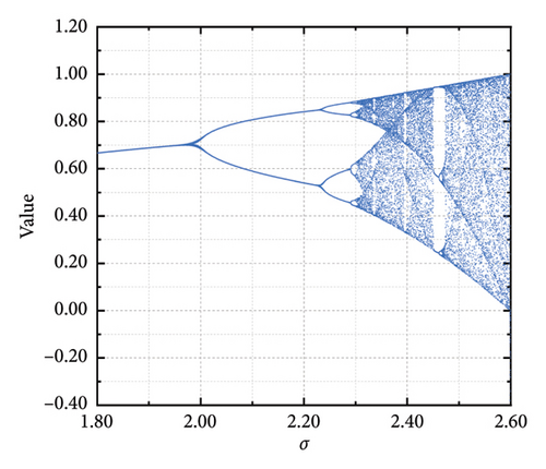
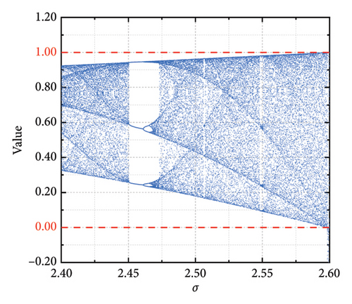
Assuming an initial value of β₁ = 0.1, the value of the parameter σ is determined using the bifurcation diagram of the cubic chaotic mapping. Taking σ as the horizontal axis, the parameter space is divided into 1000 segments. For each σ within the range [1.8, 2.6], the value of β is iterated 100 times. By sweeping through the entire parameter range, the bifurcation diagram of the cubic chaotic mapping is obtained, as shown in Figure 1(a). Figure 1(b) presents a local zoomed-in bifurcation diagram for σ within the range [2.4, 2.6]. It can be observed that when σ = 2.59, the generated values lie within the range [0, 1], which aligns with the search space of the SDI problem. Upon testing, it is found that the values yielded by the cubic chaotic mapping in one dimension exhibit good chaotic traversal properties when β₁ = 0.1 and σ = 2.59.

Details are in the caption following the image — **Figure 1 (a)**
Open in figure viewer PowerPoint

Bifurcation diagram of cubic chaotic mapping. (a) Global view. (b) Local view.

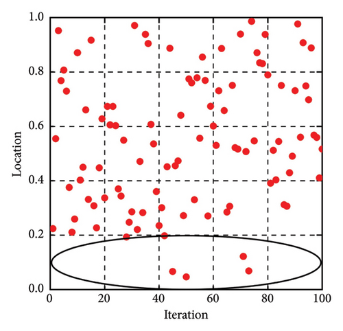
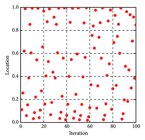
The distributions of the cubic chaotic mapping sequence and pseudo-random sequence are given in Figure 2. The number of iterations for both methods is set as 100, and the search space is between [0, 1]. Compared with the pseudo-random sequence, the cubic chaotic mapping sequence is unevenly distributed and most of the generated values tend to concentrate near the lower bound of the search space. This kind of distribution is more applicable to optimizing the problem of identifying minor damages. The β₁ is iterated (n − 1) times in each dimension according to equation (10) to accomplish the initialization in the improved algorithm.

3.2.2. WOA

The WOA is a swarm intelligence optimization algorithm that simulates the foraging behavior of humpback whales [31]. A random search mechanism in the WOA is employed in the exploration phase of the SCSO algorithm to enhance the global search ability. During the search phase, humpback whales conduct random searches based on each other’s position, which can be expressed as

()

where y_k,q and

denote the current and the next updated positions of the kth individual in the qth dimension, respectively; y_rand,q represents a randomly selected individual in the qth dimension; a decreases linearly from 2 to 0 during the iteration; and A is a random value between [−a, a] and the value of C is between [0, 2].

For better controlling the iteration process, a proper inertia weight is added to the random search mechanism [51]. Based on the sigmoid function, a curvilinear decreasing inertia weight w is adopted to the position updating equation. Moreover, the number of variables in the improved algorithm is reduced by substituting a and C, utilizing the parameters in the SCSO algorithm. The improved random search mechanism can be given as follows:

()

where Y_k,q and

denote the current and the updated positions of the kth individual in the qth dimension, respectively; Y_rand,q is a randomly selected individual in the qth dimension; t and iter_max represent the current and maximum numbers of iterations, respectively; r and r_G are the sensitivity parameters; and w decreases in the range of (0, 1).

3.2.3. Lens Opposition-Based Learning

The lens opposition-based learning (LOBL) [52] is applied in the exploration phase of the SCSO algorithm to overcome the disappearance of population diversity and search stagnation. The strategy is used to determine the individual opposite position based on the principle of convex lens imaging. The LOBL in the one-dimensional spatial is shown in Figure 3, and the search range is assumed to be [

]. The height of an individual P is h, and the projection of P on the x-axis is the individual current position X_k,q. A convex lens is placed at the center of the search range and oriented parallel to the y-axis. An inverted solid image P^′ of height h^′ is formed on the opposite side of the convex lens. The projection of P^′ on the x-axis is the generated opposite position

. Let the parameter λ = h/h^′. When λ < 1,

is closer to the convex lens; conversely,

is farther from the convex lens. In the study, λ is set as 1.2 to assist the algorithm in escaping local optima. If X_k,q and the middle value of the search space γ are used as boundaries of the search range, a new LOBL strategy can be developed as

()

where the new position

facilitates the algorithm to jump out of search stagnation. During the exploration phase, the strategy for updating the position is determined by a random number rand between [0, 1]. In the exploration phase, the position update method mainly uses the improved random search mechanism, while the LOBL performs an auxiliary search process. For simulating this search strategy, a random parameter rand with a value chosen from [0, 1] is utilized to determine the method to be adopted in each iteration. If rand ≤ 0.8, the position is updated by equation (14). Otherwise, the position can be updated according to equation (16).

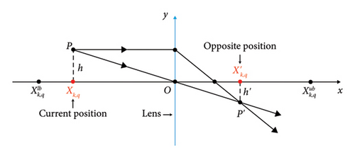
3.2.4. Stochastic Differential Mutation

Inspired by the mutation strategy of the differential evolution algorithm [53], a stochastic differential mutation strategy is proposed to overcome the issue of premature convergence in the exploitation phase of the SCSO algorithm. In the strategy, a new position of a sand cat in the qth dimension is generated by performing an operation of stochastic differential mutation utilizing the current sand cat Z_k,q, the current best individual Z_best,q, and a randomly selected individual in the population Z_rand,q. The mutation strategy helps the algorithm have better population diversity and improve its convergence accuracy. The developed strategy for stochastic differential mutation can be expressed as

()

where Z_best,q facilitates the algorithm accurately converging to the optimal solution; Z_rand,q is utilized to prevent search stagnation and expand the exploitation area; and V_k,q is a random value between [0, 1]. The influence of Z_best,q and Z_rand,q is randomly modulated by V_k,q obtained from the pseudo-random distribution, which can aid in achieving a balance between accurately converging and avoiding stagnation. During the exploitation phase, the strategy for updating the position is selected by a random number rand between 0 and 1. In line with the exploration phase, in the exploitation phase, a parameter rand with a random value generated from [0, 1] regulates the process of method selection in each iteration between the exploitation strategy of the SCSO and the stochastic differential mutation. If rand ≤ 0.8, the position is updated by equation (8). Otherwise, the position can be updated according to equation (17).

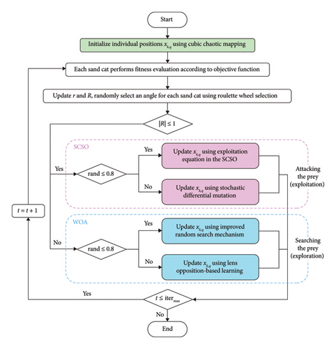
Through these improvements mentioned above, a new algorithm is developed named the W-SCSO algorithm based on the SCSO algorithm. The flowchart of the new algorithm is shown in Figure 4. It is worth noting that the algorithm chooses only one of the methods to update the position of individuals through simple judgments in each iteration. The iterative strategy does not generate much complexity in the calculation.

3.3. Benchmark Function Test

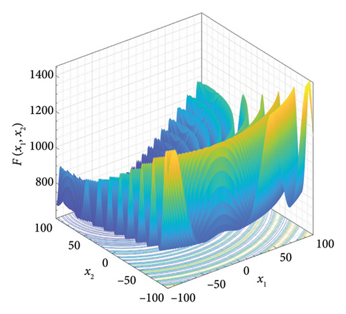
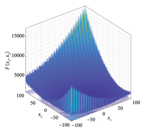
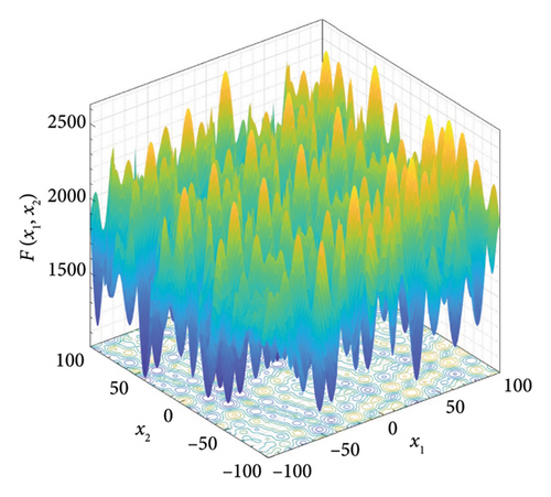
Five multimodal benchmark functions from CEC2017 have been selected for testing the exploration and exploitation ability of the W-SCSO algorithm [54]. The search domain and global minimum value f_min are presented in Table 1.

Table 1. Details of five multimodal functions.

F	Benchmark function	Domain	f_min
1	Shifted and rotated expanded Scaffer’s F6 function	[−100, 100]	600
2	Shifted and rotated Lunacek Bi_Rastrigin function		700
3	Shifted and rotated noncontinuous Rastrigin’s function		800
4	Shifted and rotated Levy function		900
5	Shifted and rotated Schwefel’s function		1000

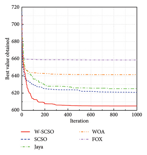
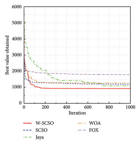
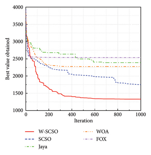
In the study, simulations are performed using MATLAB 2020b software (MathWorks, US) on the Core i7-8700 processor with 32 GB of RAM computer. The proposed algorithm is compared with the SCSO algorithm [43], Jaya algorithm (Jaya) [55], WOA [31], and Fox optimizer (FOX) [56] to show its superior optimization performance. The parameters for each optimization algorithm are shown in Table 2. The number of individuals for all algorithms is set as 30, and the maximum of iterations is set as 500. The dimension of each benchmark function is set to 10, with additional tests conducted for F1, F2, and F3 at a dimension of 30. Both algorithms are calculated 10 times for each benchmark function to acquire the best value, mean, and standard deviation of the results, and the better values between algorithms are highlighted in bold in Table 3. The convergence process of five algorithms for three typical benchmark functions in a 10-dimensional space is shown in Figure 5. According to Table 3 and Figure 5, the best value and mean of the results obtained by the proposed algorithm are lower than those of other algorithms, and the W-SCSO algorithm maintains a low standard deviation, indicating better computational accuracy and stability. Considering that the proposed algorithm maintains good accuracy and stability without significantly increasing computational complexity, it demonstrates higher efficiency compared to other algorithms. The simulation results demonstrate that the new algorithm outperforms the other four algorithms in terms of both convergence efficiency and calculation accuracy.

Table 2. Parameters of each optimization algorithm.

Algorithm	Parameter	Value
W-SCSO	Sensitivity range (r_G)	[0, 2]
	Random angle (θ)	[0, 360]
	A^′	[0, 2]
	λ	1.2

SCSO	Sensitivity range (r_G)	[0, 2]
SCSO	Random angle (θ)	[0, 360]

Jaya	Without algorithm-specific control parameters


WOA	a	[0, 2]
	A	[0, 2]
	l	[−1, 1]
	C	2·rand (0, 1)
	b	1

FOX	c₁	0.18
	c₂	0.19
	Time_S_T_it	[0, 1]

Table 3. Simulation results of five multimodal functions.

F	Dimension	Result	W-SCSO	SCSO	Jaya	WOA	FOX
1	10	Best	602.95	609.37	620.88	625.71	651.57
		Mean	605.08	620.86	625.21	641.50	658.52
		Standard deviation	1.77	7.43	5.41	10.01	5.13
	30	Best	637.46	648.25	674.18	652.96	664.09
		Mean	639.72	662.73	689.63	672.54	666.59
		Standard deviation	1.32	8.72	14.78	18.74	1.68

2	10	Best	733.37	785.68	764.44	755.31	811.27
		Mean	738.29	790.61	783.16	768.48	818.79
		Standard deviation	4.10	3.71	11.73	8.91	8.92
	30	Best	957.99	1170.7	1284.9	1332	1283.1
		Mean	986.91	1259.23	1417.08	1359.43	1311.78
		Standard deviation	22.89	85.07	93.88	20.14	23.41

3	10	Best	811.28	826.37	838.77	830.63	833.83
		Mean	813.71	827.53	853.20	843.06	848.75
		Standard deviation	1.94	0.73	13.32	7.74	21.95
	30	Best	941.76	964.04	1126.10	999.59	990.04
		Mean	953.33	1002.06	1157.20	1012.47	1010.93
		Standard deviation	15.27	26.56	19.49	13.49	26.11

4	10	Best	900.56	1008.00	1063.20	1136.40	1742.20
		Mean	913.33	1185.73	1088.98	1256.68	1781.65
		Standard deviation	20.57	200.69	32.85	123.63	34.34

5	10	Best	1172.10	1522.70	2301.40	1835.60	1934.70
		Mean	1328.58	1749.03	2388.98	2275.03	2535.98
		Standard deviation	96.53	210.75	54.54	363.54	443.86

4. Numerical Simulations

In this section, a simply supported beam is employed for numerical simulations to assess the effectiveness of the proposed SDI method in bridge structure. Gaussian white noise is randomly added to interfere with the modal data for accurately simulating the impact of uncertain measurement noise on practical measurement data [57, 58]. The interference can give randomness to the influence of noise appearing at any moment, which can be expressed as

()

where τ_noise and τ₀ represent the modal parameter value with and without noise interference, respectively; ε denotes the degree of noise interference; and R_τ is a generated random number subjected to the standard normal distribution.

To illustrate the advantages of the improved objective function, it will be compared to the traditional objective function constructed based on FCR and MAC [29], defined as obj 2:

()

where

and

represent the calculated and measured mode shape vectors of the ith order, respectively. The superscript T indicates the transpose operation applied to the vector; and MN denotes the number of measured nodes.

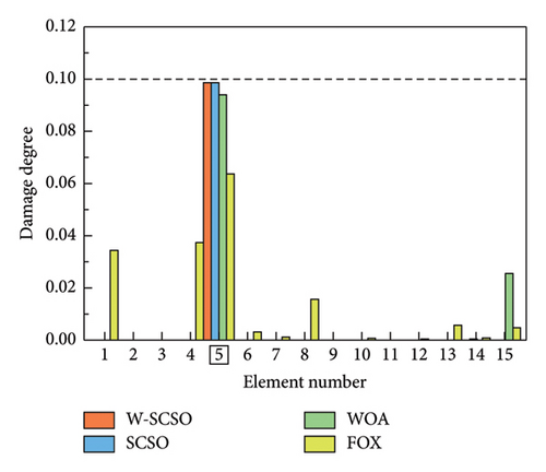
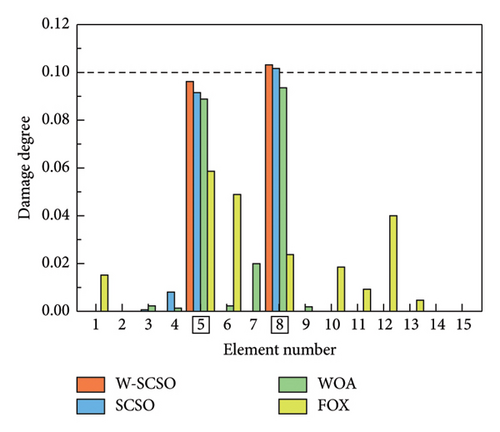
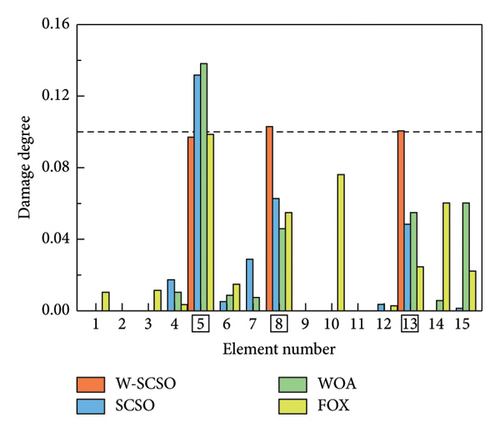
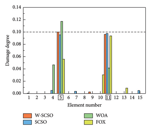
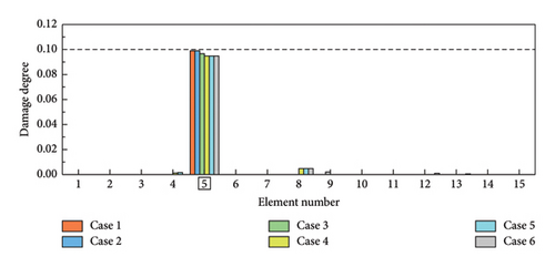
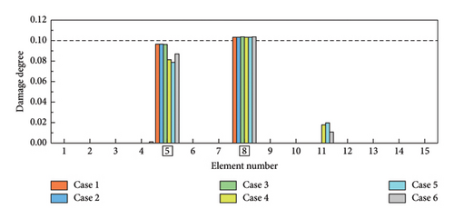
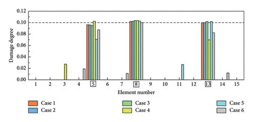
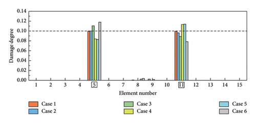
The FE model of a simply supported beam is composed of 15 elements and 14 measured nodes, as shown in Figure 6. The left support of the beam is completely fixed, and the right support is constrained in vertical freedom. Deformation along the axial direction of the beam is neglected in the simulation. Vertical DOFs are measured at the nodes on the beam. Two scenarios with different sensor configurations were considered. When 14 DOFs are measured, sensors are placed at all nodes, while for 7 DOFs, sensors are positioned at nodes 1, 3, 5, 7, 9, 11, and 13. The length and Young’s modulus of the beam are set as 6.00 m and 70 GPa, respectively. The rectangular sectional area, density, and moment of sectional inertia are defined as 3.00 × 10⁻² m², 2750 kg/m³, and 1.10 × 10⁻⁵ m⁴, respectively. Figure 7 illustrates the first-order MSC of the simply supported beam in different damage elements with a 10% degree of damage in a noise-free condition. It can be found that the MSC at the location of the intact element remains smooth, whereas the MSC at the damaged element changes significantly. In order to locate and quantify structural damage effectively, the first five modal data of the structure are selected for both obj 1 and obj 2 in simulations [20]. The W-SCSO algorithm, SCSO algorithm [43], WOA [31], and FOX [56] are applied in simulations. The initial number of individuals for four algorithms is set as 30, and the maximum number of iterations is set as 100. Each damage case is calculated 30 times to avoid singularity results. Subsequently, the result with the lowest fitness value is obtained to determine the effective SDI consequence.

To acquire the optimal performance of the improved objective function, different regularization parameters ϵ are selected for analysis. The triple damage of the simply supported beam is used as a case study, and the W-SCSO algorithm along with obj 1 is employed for computation. Table 4 shows the SDI results with different regularization parameters. The symbol “5@10%” in Table 4 indicates that the stiffness of element “5” has been decreased by “10%.” The symbol “0.15%&5%” represents a noise level of ±0.15% in natural frequencies and ±5% in mode shape data [58]. Results show that when ϵ = 0.001, the SDI result achieves the highest accuracy without any misidentifications compared to other parameters. Therefore, ϵ = 0.001 is used to improve the robustness of both obj 1 and obj 2 in the simulations.

Table 4. Damage identification results with different regularization parameters.

ϵ	Damage element	Noise level	Identified damage	Misidentification
0	5@10%, 8@10%, 13@10%	0.15%&5%	[email protected]%, [email protected]%, [email protected]%	[email protected]%
0.0001			[email protected]%, [email protected]%, [email protected]%	[email protected]%
0.001			[email protected]%, [email protected]%, [email protected]%	None
0.01			[email protected]%, [email protected]%, [email protected]%	None
0.1			[email protected]%, [email protected]%, [email protected]%	[email protected]%
1			[email protected]%, [email protected]%, [email protected]%	[email protected]%

As shown in Table 5, six distinct cases are applied for the simulations of single, double, triple, and symmetrical damages. In cases 1–3, obj 1 is used for SDI, while obj 2 is employed in cases 4–6. The SDI results are shown in Figures 8 and 9. The labels of the actual damaged elements are framed, and the actual degree of damage is marked with a dashed line. On the one hand, the proposed W-SCSO algorithm produces higher precision and less degree of misidentifications compared to the other algorithms in these simulations. On the other hand, compared to obj 2, the proposed obj 1 can more accurately locate and quantify structural damages, which exhibits stronger noise robustness. Especially in triple damage cases, obj 2 struggles to accurately quantify the damage degree of multiple damaged elements, while obj 1 is sensitive to multiple damages, even under high level noise interference. The accuracy of the identification using obj 2 in symmetrical damage cases is reduced because the natural frequency, or circular frequency, sensitivities between symmetric parameters are always equal when damages occur in a symmetric structure with symmetrical form and degree [59]. On the contrary, obj 1 can effectively restrict the adverse effect of natural frequency sensitivities in symmetrical damage identification. Based on the W-SCSO algorithm and the improved objective function, the proposed method has been successfully validated for accurately identifying structural damage in both single and multiple damages using incomplete modal data, even with strong noise interference.

Table 5. Different cases of damage identification for simply supported beam.

Case	Measured DOFs	Objective function	Noise level	Damage degree
1	14	obj 1 (MSC & FCR & L_1/2 sparse regularization)	0.15%&5%	10%
2	14		0.15%&10%
3	7		0.15%&10%
4	14	obj 2 (MAC & FCR & L_1/2 sparse regularization)	0.15%&5%
5	14		0.15%&10%
6	7		0.15%&10%

5. Experimental Verification

5.1. Experimental Setup and Finite Element Model Updating

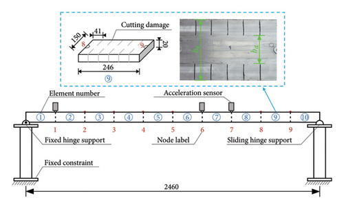
A simply supported beam model made of aluminum alloy was constructed in the laboratory to evaluate the effectiveness of the proposed method. The geometric parameters and boundary conditions of the beam model are shown in Figure 10, and the experimental model and instruments applied in the experiment are shown in Figure 11. The acceleration responses are collected using the DH5922 dynamic signal test system. The data collection method is preset to continuous sampling, and the signal sampling frequency, the number of time domain points, and the sampling time of each case are 1000 Hz, 2048, and 60 s, respectively. The length and moment of sectional inertia of the beam are defined as 2.46 m and 1.00 × 10⁻⁷ m⁴, respectively. The initial sectional area, density, and Young’s modulus of the beam are 3.00 × 10⁻³ m², 2750 kg/m³, and 70 GPa, respectively.

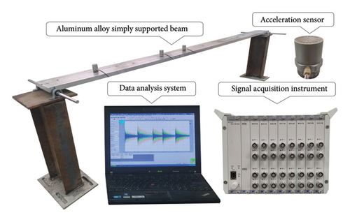
The modal information of the beam is obtained by hammer impact testing for FE model updating and SDI. Three piezoelectric acceleration sensors with the INV9828 specification and a voltage sensitivity of 50.047 mV/ms⁻² are placed at nodes to measure the vertical acceleration responses. The sensor located at the first node is fixed, and the remaining sensors are moved in turn from the second node to the ninth node to measure the response data. Subsequently, acceleration responses of the beam are obtained by conducting normalization and the Fast Fourier Transform method is utilized to precondition the responses [60]. Then, the data analysis system is used to obtain the mode shapes and natural frequencies of the experimental beam.

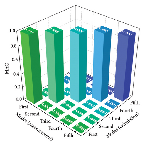
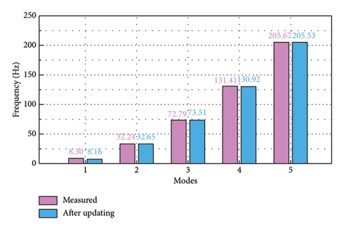
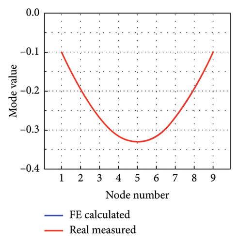
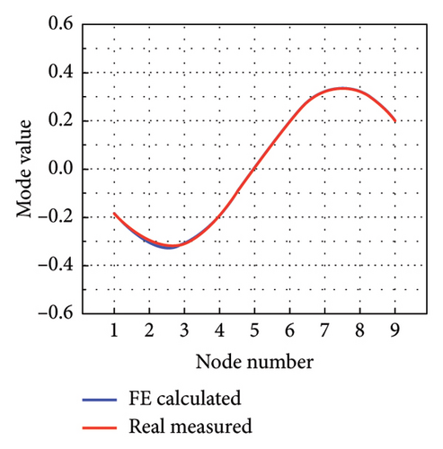
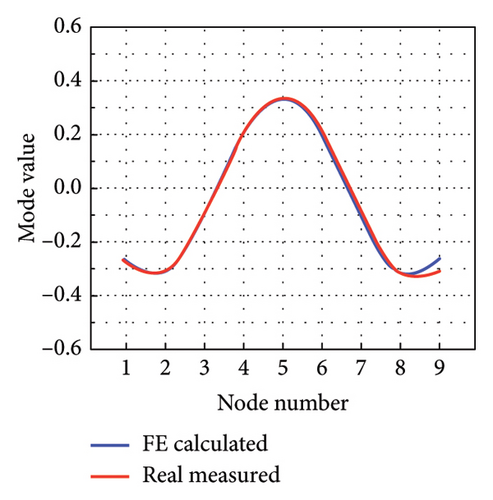
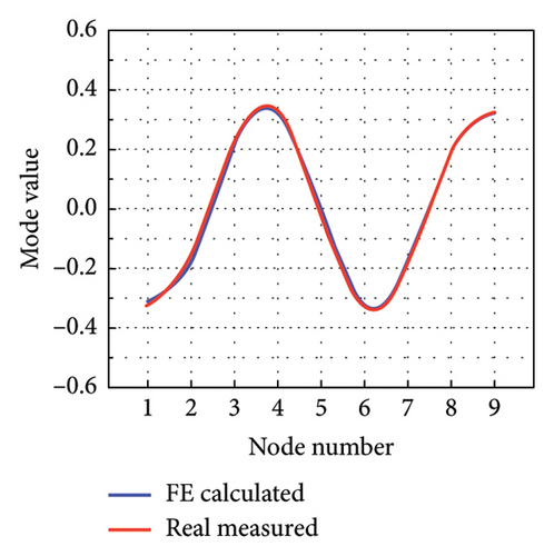
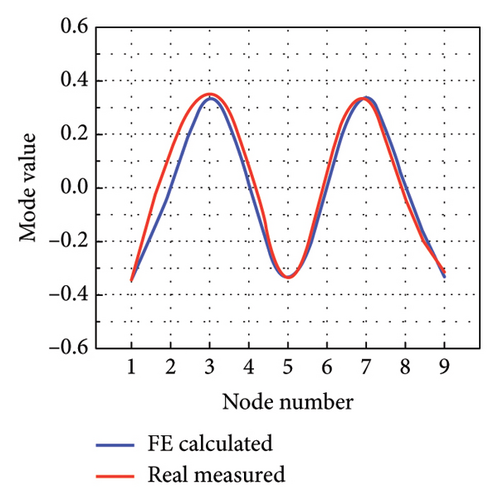
The intact experimental beam is measured five times, and the average of the measured data serves as the measured response for model updating. The limited number of sensors causes the issue of structural modal incompleteness; thereby, Guyan reduction scheme is utilized to acquire low-order modes of the FE model. The W-SCSO algorithm and the improved objective function are utilized for model updating. The updated sectional area, density, moment of sectional inertia, and Young’s modulus of the beam are 2.81 × 10⁻³ m², 2683 kg/m³, 1.002 × 10⁻⁷ m⁴, and 7.32 × 10¹⁰ N/m², respectively. The accuracy of the updated FE model can be verified by comparing the measured and calculated MAC, natural frequencies, and mode shapes from the first one to the five orders [20], as shown in Figures 12 and 13. It is obvious that, after model updating, the correlation values of the same orders along the diagonal line in the MAC tend to be 1 and the other values tend to be 0, indicating a strong correlation between modes of the same order in the measured and calculated data. Furthermore, the measured and calculated natural frequencies and mode shapes exhibit similarities. Hence, the calculated results of the updated model have been validated to be consistent with the experimental measurements.

5.2. Experimental Process and Damage Identification

Symmetric cutting damage is employed to simulate the reduction of stiffness within the specified element, as shown in Figure 10 [37, 61]. Without taking into account the loss of mass, the change in flexural stiffness is simulated by reducing the cross-sectional moment of inertia. The SDI factor α in the experiment is calculated as

()

where

and

represent the moment of inertia of the cross section in the intact and damaged states, respectively; b_e and b_d represent the widths of the cross section before and after cutting, respectively; and h_e and h_d represent the height of the cross section before and after cutting, respectively.

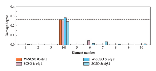
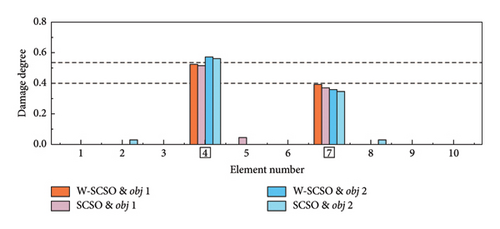
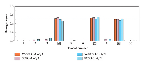
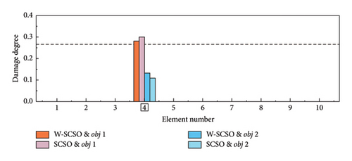
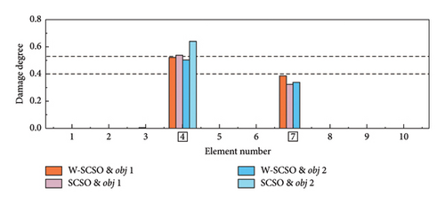
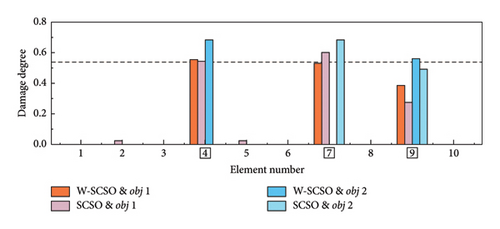
In the experiment, three damage cases are set up, as detailed in Table 6. SDI is performed based on the first four orders of modal information. Each damage case was measured five times, and the average of the measured data was calculated to serve as the reference results. It is worth noting that the measurement data were inevitably interfered with noise, which can lead to uncertain measurement errors and impact the accuracy of the SDI. The reference results are inputted into the W-SCSO and SCSO algorithms to independently calculate the consequence based on obj 1 and obj 2 separately. In this section, the number of individuals for both algorithms is set as 30, with a maximum of 100 iterations.

Table 6. Damage cases of W-SCSO and SCSO algorithms for experimental beam.

Case	Damage element	Depth of cut (cm)	Damage degree (%)
1	4	4	26.67

2	4	8	53.33
2	7	6	40.00

3	4	8	53.33
	7	8	53.33
	9	8	53.33

To select an appropriate regularization parameter ϵ and compare the numerical and experimental results, SDI is conducted using the updated FE model of the experimental beam, with damage cases consistent with those presented in Table 6. Table 7 shows the SDI results for case 3 under different regularization parameters, where the W-SCSO algorithm with obj 1 is applied for computation. The results indicate that when ϵ = 0.05, the SDI results achieve the highest accuracy compared to other parameter values. Thus, the regularization parameter ϵ is set as 0.05 for obj 1 and obj 2 in the subsequent numerical simulations and experiments.

Table 7. Damage identification results of experimental beam with different regularization parameters.

ϵ	Noise level	Identified damage	Misidentification
0	0.15%&5%	[email protected]%, [email protected]%, [email protected]%	[email protected]%, [email protected]%
0.005		[email protected]%, [email protected]%, [email protected]%	[email protected]%
0.01		[email protected]%, [email protected]%, [email protected]%	[email protected]%
0.05		[email protected]%, [email protected]%, [email protected]%	None
0.1		[email protected]%, [email protected]%, [email protected]%	None
0.5		[email protected]%, [email protected]%, [email protected]%	None
1		[email protected]%, [email protected]%, [email protected]%	None

In both the numerical model and experimental beam, the W-SCSO and SCSO algorithms are, respectively, applied to compute each damage case 20 times, with the SDI results corresponding to the lowest fitness values shown in Figures 14 and 15. Specially, in the numerical simulation, a noise level of ±0.15% in natural frequencies and ±5% in mode shape data are added. The simulation results demonstrate that the use of obj 1 enables accurate damage identification of the updated FE model, exhibiting stronger robustness compared to obj 2. Furthermore, the proposed W-SCSO algorithm outperforms the SCSO algorithm, achieving fewer misidentifications and higher accuracy in SDI. When using the experimental beam model for damage identification, both algorithms struggle to accurately identify the actual triple damage when employing obj 2. Nevertheless, the proposed obj 1 can be used to identify single and multiple damages. The W-SCSO algorithm can effectively optimize the objective function for locating and quantifying actual damages, whereas the SCSO algorithm tends to produce more errors and misidentifications. The reasons for the imprecise SDI results lie in the random noise disturbance, measurement and model errors, and modal incompleteness. Comparative outcomes indicate that the proposed method possesses strong robustness and satisfactory sensitivity to damage. Experimental results proved that the proposed SDI method, which combines the W-SCSO algorithm and the improved objective function, effectively use the first four orders of incomplete modal information to identify single and multiple damages in the experimental beam. Therefore, the developed approach can be considered to have good applicability in addressing damage identification in bridge structures.

6. Conclusions

In this study, a W-SCSO method is proposed for damage identification. Through simulations and experimental studies, some of the conclusions can be drawn as follows:

1.
Better optimization ability and stability of the W-SCSO algorithm are demonstrated compared with the other four algorithms through the CEC2017 benchmark function test. Results indicate that the W-SCSO algorithm exhibits both computational stability and high accuracy.
2.
Numerical simulations are performed to verify the effect of the proposed SDI method based on the W-SCSO algorithm and the improved objective function. The simulation results demonstrate that this method can effectively address the SDI problem using incomplete modal data, which represents stronger robustness in the presence of high noise interference.
3.
Damage identification results from both numerical and experimental studies show that the proposed method exhibits excellent accuracy and effectiveness in locating and quantifying damages within bridge structures, even with modal incompleteness and strong noise interference.

Conflicts of Interest

The authors declare no conflicts of interest.

Funding

This work was jointly supported by the National Natural Science Foundation of China (Grant Number U2004184), China Scholarship Council Fund as a Senior Research Fellow (Grant Number 202308410481), Training Plan for Young Key Teachers in Colleges and Universities in Henan Province, China (Grant Number 2021GGJS078), CRSRI Open Research Program (Grant Number CKWV20241182/KY), Key Scientific and Technological Research Projects of Henan Province, China (242102241015), and Henan Provincial Natural Science Foundation Project (Grant Number 252300420048).

Open Research

Data Availability Statement

The data that support the findings of this study are available from the corresponding author upon reasonable request.

References

1 Sun H. S., Song L., and Yu Z. W., A Deep Learning-Based Bridge Damage Detection and Localization Method, Mechanical Systems and Signal Processing. (2023) 193, https://doi.org/10.1016/j.ymssp.2023.110277.
10.1016/j.ymssp.2023.110277
Web of Science® Google Scholar
2 Hou R. R. and Xia Y., Review on the New Development of Vibration-Based Damage Identification for Civil Engineering Structures: 2010–2019, Journal of Sound and Vibration. (2021) 491, https://doi.org/10.1016/j.jsv.2020.115741.
10.1016/j.jsv.2020.115741
Web of Science® Google Scholar
3 Qin L. F., Ren W. X., and Yan W. J., Sensitive Properties of Power Spectral Density Transmissibility (PSDT) to Moving Vehicles and Structural States in Bridge Health Monitoring, Structural Control and Health Monitoring. (2024) 2024, no. 1, https://doi.org/10.1155/2024/4695910.
10.1155/2024/4695910
Web of Science® Google Scholar
4 Nsengiyumva W., Zhong S. C., Lin J. W., Zhang Q. K., Zhong J. F., and Huang Y. X., Advances, Limitations and Prospects of Nondestructive Testing and Evaluation of Thick Composites and Sandwich Structures: A State-of-The-Art Reviewlimitations and Prospects of Nondestructive Testing and Evaluation of Thick Composites and Sandwich Structures: A State-of-The-Art Review, Composite Structures. (2021) 256, https://doi.org/10.1016/j.compstruct.2020.112951.
10.1016/j.compstruct.2020.112951
Google Scholar
5 Yang Y., Lu H. C., Tan X. K., Wang R. Q., and Zhang Y., Mode Shape Identification and Damage Detection of Bridge by Movable Sensory System, IEEE Transactions on Intelligent Transportation Systems. (2023) 24, no. 1, 1299–1313, https://doi.org/10.1109/tits.2022.3151529.
10.1109/TITS.2022.3151529
Web of Science® Google Scholar
6 Khedmatgozar Dolati S. S., Malla P., Ortiz J. D., Mehrabi A., and Nanni A., Identifying NDT Methods for Damage Detection in Concrete Elements Reinforced or Strengthened With FRP, Engineering Structures. (2023) 287, https://doi.org/10.1016/j.engstruct.2023.116155.
10.1016/j.engstruct.2023.116155
Google Scholar
7 Manoach E., Warminski J., Kloda L., and Teter A., Numerical and Experimental Studies on Vibration Based Methods for Detection of Damage in Composite Beams, Composite Structures. (2017) 170, 26–39, https://doi.org/10.1016/j.compstruct.2017.03.005, 2-s2.0-85015622557.
10.1016/j.compstruct.2017.03.005
Web of Science® Google Scholar
8 Hassani S., Structural Damage Detection Using Mutual Information and Improved Reptile Search Algorithm for Fused Smooth Signals Affected by Coloured Noise, Structural Control and Health Monitoring. (2024) 2024, no. 1, https://doi.org/10.1155/2024/8925127.
10.1155/2024/8925127
Web of Science® Google Scholar
9 Lu Z. R., Zhou J. X., Wang L., and Liu J. K., Damage Identification From Static Tests by Eigenparameter Decomposition and Sparse Regularization, Structural Health Monitoring. (2020) 19, no. 5, 1351–1374, https://doi.org/10.1177/1475921719880980.
10.1177/1475921719880980
Web of Science® Google Scholar
10 Le N. T., Thambiratnam D. P., Nguyen A., and Chan T. H. T., A New Method for Locating and Quantifying Damage in Beams From Static Deflection Changes, Engineering Structures. (2019) 180, 779–792, https://doi.org/10.1016/j.engstruct.2018.11.071, 2-s2.0-85057581932.
10.1016/j.engstruct.2018.11.071
Web of Science® Google Scholar
11 Roustazadeh S. and Daneshjoo F., Damage Identification of Multi-Span Bridges Using a Novel Damage Index Based on a New Algorithm for Prediction of Healthy State Displacement, International Journal of Structural Stability and Dynamics. (2023) 23, no. 19, https://doi.org/10.1142/s0219455423501894.
10.1142/S0219455423501894
Web of Science® Google Scholar
12 Yin T., Jiang Q. H., and Yuen K. V., Vibration-Based Damage Detection for Structural Connections Using Incomplete Modal Data by Bayesian Approach and Model Reduction Technique, Engineering Structures. (2017) 132, 260–277, https://doi.org/10.1016/j.engstruct.2016.11.035, 2-s2.0-84999027838.
10.1016/j.engstruct.2016.11.035
Web of Science® Google Scholar
13 Zhou X., Kim C. W., Zhang F. L., and Chang K. C., Vibration-Based Bayesian Model Updating of an Actual Steel Truss Bridge Subjected to Incremental Damage, Engineering Structures. (2022) 260, https://doi.org/10.1016/j.engstruct.2022.114226.
10.1016/j.engstruct.2022.114226
Web of Science® Google Scholar
14 Cao L., He W. Y., and Ren W. X., Damage Localization and Quantification for Beam Bridges Based on Frequency Variation of Parked Vehicle-Bridge Systems, Structures. (2021) 31, 357–368, https://doi.org/10.1016/j.istruc.2021.01.098.
10.1016/j.istruc.2021.01.098
Web of Science® Google Scholar
15 Chen S. C., Zheng X. J., Yang X. J., Zheng T., Yang B., and Lei Y., Structural Damage Detection Based on Structural Macro-Strain Mode Shapes Extracted From Non-Stationary Output Responses, Measurement Science and Technology. (2024) 35, no. 9, https://doi.org/10.1088/1361-6501/ad4c85.
10.1088/1361-6501/ad4c85
PubMed Web of Science® Google Scholar
16 Shadan F., Khoshnoudian F., and Esfandiari A., Structural Damage Identification Based on Strain Frequency Response Functions, International Journal of Structural Stability and Dynamics. (2018) 18, no. 12, https://doi.org/10.1142/s0219455418501596, 2-s2.0-85052954320.
10.1142/s0219455418501596
Web of Science® Google Scholar
17 Jahangiri M., Hadianfard M. A., Najafgholipour M. A., and Jahangiri M., Vibration-Based Structural Damage Detection Using the Interactive Autodidactic School Optimization Algorithm Based on an Energy-Dissipation Method, International Journal of Structural Stability and Dynamics. (2022) 22, no. 16, https://doi.org/10.1142/s0219455422501929.
10.1142/s0219455422501929
Web of Science® Google Scholar
18 Xie D. X., Lu Z. R., Li G., Liu J. K., and Wang L., Efficient Laplace Prior-Based Sparse Bayesian Learning for Structural Damage Identification and Uncertainty Quantification, Mechanical Systems and Signal Processing. (2023) 188, https://doi.org/10.1016/j.ymssp.2022.110000.
10.1016/j.ymssp.2022.110000
Web of Science® Google Scholar
19 Gomes G. F. and Giovani R. S., An Efficient Two-Step Damage Identification Method Using Sunflower Optimization Algorithm and Mode Shape Curvature (MSDBI-SFO), Engineering With Computers. (2022) 38, no. 2, 1711–1730, https://doi.org/10.1007/s00366-020-01128-2.
10.1007/s00366-020-01128-2
Web of Science® Google Scholar
20 Chen Z., Wang Y. K., Zhang K., Chan T. H. T., and Wang Z. H., Damage Detection and Location Using a Simulated Annealing-Artificial Hummingbird Algorithm With an Improved Objective Function, Structural Health Monitoring. (2025) 24, no. 1, 129–147, https://doi.org/10.1177/14759217241233733.
10.1177/14759217241233733
Web of Science® Google Scholar
21 Padil K. H., Bakhary N., Abdulkareem M., Li J., and Hao H., Non-Probabilistic Method to Consider Uncertainties in Frequency Response Function for Vibration-Based Damage Detection Using Artificial Neural Network, Journal of Sound and Vibration. (2020) 467, https://doi.org/10.1016/j.jsv.2019.115069.
10.1016/j.jsv.2019.115069
Web of Science® Google Scholar
22 Cheng C. M., Zhao B. X., Fu C. K., Peng Z. K., and Meng G., A Two-Stage Sparse Algorithm for Localization and Characterization of Local Nonlinear Structures, Journal of Sound and Vibration. (2022) 526, https://doi.org/10.1016/j.jsv.2022.116823.
10.1016/j.jsv.2022.116823
Web of Science® Google Scholar
23 Hou R. R., Xia Y., and Zhou X. Q., Structural Damage Detection Based on L1 Regularization Using Natural Frequencies and Mode Shapes, Structural Control and Health Monitoring. (2017) 25, no. 3, e2107–e2117, https://doi.org/10.1002/stc.2107, 2-s2.0-85041668017.
10.1002/stc.2107
Google Scholar
24 Zhu H. P., Yu H., Gao F., Weng S., Sun Y., and Hu Q., Damage Identification Using Time Series Analysis and Sparse Regularization, Structural Control and Health Monitoring. (2020) 27, no. 9, https://doi.org/10.1002/stc.2554.
10.1002/stc.2554
Web of Science® Google Scholar
25 Bao Y. Q., Li H., and Ou J. P., Emerging Data Technology in Structural Health Monitoring: Compressive Sensing Technology, Journal of Civil Structural Health Monitoring. (2014) 4, no. 2, 77–90, https://doi.org/10.1007/s13349-013-0064-1, 2-s2.0-84896322382.
10.1007/s13349-013-0064-1
Google Scholar
26 Thankachan P., Fida A., and Pillai T. M. M., Health Monitoring of Steel Structures Using Cuckoo Search Algorithm-Based ANN, Structures. (2024) 61, https://doi.org/10.1016/j.istruc.2024.105933.
10.1016/j.istruc.2024.105933
Web of Science® Google Scholar
27 Minh H. L., Sang-To T., Abdel Wahab M., and Cuong-Le T., A New Metaheuristic Optimization Based on K-Means Clustering Algorithm and Its Application to Structural Damage Identification, Knowledge-Based Systems. (2022) 251, https://doi.org/10.1016/j.knosys.2022.109189.
10.1016/j.knosys.2022.109189
Web of Science® Google Scholar
28 Zhang G. C., Wan C. F., Xiong X. B., Xie L. Y., Noori M., and Xue S. T., Output-only Structural Damage Identification Using Hybrid Jaya and Differential Evolution Algorithm With Reference-Free Correlation Functions, Measurement. (2022) 199, https://doi.org/10.1016/j.measurement.2022.111591.
10.1016/j.measurement.2022.111591
Web of Science® Google Scholar
29 Ding Z. H., Li J., and Hao H., Structural Damage Identification Using Improved Jaya Algorithm Based on Sparse Regularization and Bayesian Inference, Mechanical Systems and Signal Processing. (2019) 132, 211–231, https://doi.org/10.1016/j.ymssp.2019.06.029, 2-s2.0-85067839262.
10.1016/j.ymssp.2019.06.029
Web of Science® Google Scholar
30 Chen Z., Zhang K., Chan T. H. T., Li X. K., and Zhao S. B., A Novel Hybrid Whale-Chimp Optimization Algorithm for Structural Damage Detection, Applied Sciences. (2022) 12, no. 18, https://doi.org/10.3390/app12189036.
10.3390/app12189036
Google Scholar
31 Mirjalili S. and Lewis A., The Whale Optimization Algorithm, Advances in Engineering Software. (2016) 95, 51–67, https://doi.org/10.1016/j.advengsoft.2016.01.008, 2-s2.0-84959304045.
10.1016/j.advengsoft.2016.01.008
Web of Science® Google Scholar
32 Huang M. S., Gül M., and Zhu H. P., Vibration-Based Structural Damage Identification Under Varying Temperature Effects, Journal of Aerospace Engineering. (2018) 31, no. 3, https://doi.org/10.1061/(asce)as.1943-5525.0000829, 2-s2.0-85041716285.
10.1061/(asce)as.1943-5525.0000829
Web of Science® Google Scholar
33 Huang M. S., Ling Z. Z., Sun C. et al., Two-Stage Damage Identification for Bridge Bearings Based on Sailfish Optimization and Element Relative Modal Strain Energy, Structural Engineering & Mechanics. (2023) 86, no. 6, 715–730.
Web of Science® Google Scholar
34 Tran-Ngoc H., Khatir S., De Roeck G., Bui-Tien T., Nguyen-Ngoc L., and Abdel Wahab M., Model Updating for Nam O Bridge Using Particle Swarm Optimization Algorithm and Genetic Algorithm, Sensors. (2018) 18, no. 12, https://doi.org/10.3390/s18124131, 2-s2.0-85057534018.
10.3390/s18124131
Web of Science® Google Scholar
35 Dinh-Cong D., Truong T. T., and Nguyen-Thoi T., A Comparative Study of Different Dynamic Condensation Techniques Applied to Multi-Damage Identification of FGM and FG-CNTRC Plates, Engineering With Computers. (2022) 38, no. S5, 3951–3975, https://doi.org/10.1007/s00366-021-01312-y.
10.1007/s00366-021-01312-y
Web of Science® Google Scholar
36 Zhang J. W., Huang M. S., Wan N., Deng Z. H., He Z. G., and Luo J., Missing Measurement Data Recovery Methods in Structural Health Monitoring: The State, Challenges and Case Study, Measurement. (2024) 231, https://doi.org/10.1016/j.measurement.2024.114528.
10.1016/j.measurement.2024.114528
Web of Science® Google Scholar
37 Lei Y. Z., Li J., and Hao H., Physics-Guided Deep Learning Based on Modal Sensitivity for Structural Damage Identification With Unseen Damage Patterns, Engineering Structures. (2024) 316, https://doi.org/10.1016/j.engstruct.2024.118510.
10.1016/j.engstruct.2024.118510
Web of Science® Google Scholar
38 Huang M. S., Wan N., and Zhu H. P., Reconstruction of Structural Acceleration Response Based on CNN-BiGRU With Squeeze-And-Excitation Under Environmental Temperature Efects, Journal of Civil Structural Health Monitoring. (2024) 54, 1–19.
CAS Google Scholar
39 Huang M. S., Zhang J. W., Hu J. L., Ye Z. T., Deng Z. H., and Wan N., Nonlinear Modeling of Temperature-Induced Bearing Displacement of Long-Span Single-Pier Rigid Frame Bridge Based on DCNN-LSTM, Case Studies in Thermal Engineering. (2024) 53, https://doi.org/10.1016/j.csite.2023.103897.
10.1016/j.csite.2023.103897
Web of Science® Google Scholar
40 Tran-Ngoc H., Khatir S., Ho-Khac H., De Roeck G., Bui-Tien T., and Abdel Wahab M., Efficient Artificial Neural Networks Based on a Hybrid Metaheuristic Optimization Algorithm for Damage Detection in Laminated Composite Structures, Composite Structures. (2021) 262, https://doi.org/10.1016/j.compstruct.2020.113339.
10.1016/j.compstruct.2020.113339
Web of Science® Google Scholar
41 Huang M. S., Zhang J. W., Li J., Deng Z. H., and Luo J., Damage Identification of Steel Bridge Based on Data Augmentation and Adaptive Optimization Neural Network, Structural Health Monitoring. (2024) https://doi.org/10.1177/14759217241255042.
10.1177/14759217241255042
Web of Science® Google Scholar
42 Zheng W. H., Li J., and Hao H., Data Augmentation of Dynamic Responses for Structural Health Monitoring Using Denoising Diffusion Probabilistic Models, Engineering Structures. (2025) 328, https://doi.org/10.1016/j.engstruct.2025.119685.
10.1016/j.engstruct.2025.119685
Web of Science® Google Scholar
43 Seyyedabbasi A. and Kiani F., Sand Cat Swarm Optimization: A Nature-Inspired Algorithm to Solve Global Optimization Problems, Engineering With Computers. (2022) 39, no. 4, 2627–2651, https://doi.org/10.1007/s00366-022-01604-x.
10.1007/s00366-022-01604-x
Web of Science® Google Scholar
44 Wu D., Rao H. H., Wen C. S., Jia H. M., Liu Q. X., and Abualigah L., Modified Sand Cat Swarm Optimization Algorithm for Solving Constrained Engineering Optimization Problems, Mathematics. (2022) 10, no. 22, https://doi.org/10.3390/math10224350.
10.3390/math10224350
Web of Science® Google Scholar
45 Qiu Y. G. and Zhou J., Short-Term Rockburst Damage Assessment in Burst-Prone Mines: An Explainable XGBOOST Hybrid Model With SCSO Algorithm, Rock Mechanics and Rock Engineering. (2023) 56, no. 12, 8745–8770, https://doi.org/10.1007/s00603-023-03522-w.
10.1007/s00603-023-03522-w
Web of Science® Google Scholar
46 Kiani F., Anka F. A., and Erenel F., PSCSO: Enhanced Sand Cat Swarm Optimization Inspired by the Political System to Solve Complex Problems, Advances in Engineering Software. (2023) 178, https://doi.org/10.1016/j.advengsoft.2023.103423.
10.1016/j.advengsoft.2023.103423
Web of Science® Google Scholar
47 Talaei S., Zhu X. Q., Li J. C., Yu Y., and Chan T. H. T., Transfer Learning Based Bridge Damage Detection: Leveraging Time-Frequency Features, Structures. (2023) 57, https://doi.org/10.1016/j.istruc.2023.105052.
10.1016/j.istruc.2023.105052
Web of Science® Google Scholar
48 Guyan R. J., Reduction of Stiffness and Mass Matrices, AIAA Journal. (1965) 3, no. 2, https://doi.org/10.2514/3.2874, 2-s2.0-85007709933.
10.2514/3.2874
Web of Science® Google Scholar
49 Ding Z. H., Fu K. S., Deng W., Li J., and Zhongrong L., A Modified Artificial Bee Colony Algorithm for Structural Damage Identification Under Varying Temperature Based on a Novel Objective Function, Applied Mathematical Modelling. (2020) 88, 122–141, https://doi.org/10.1016/j.apm.2020.06.039.
10.1016/j.apm.2020.06.039
Web of Science® Google Scholar
50 Yang X. P., Min L. Q., and Wang X., A Cubic Map Chaos Criterion Theorem With Applications in Generalized Synchronization Based Pseudorandom Number Generator and Image Encryption, Chaos. (2015) 25, no. 5, https://doi.org/10.1063/1.4917380, 2-s2.0-84928910605.
10.1063/1.4917380
PubMed Web of Science® Google Scholar
51 Li J. T., Su S. Q., Wang W., Liu X. W., and Zuo F. L., Fast Reconstruction Method for Defect Profiles of Ferromagnetic Materials Based on Metal Magnetic Memory Technique, Measurement. (2023) 215, https://doi.org/10.1016/j.measurement.2023.112885.
10.1016/j.measurement.2023.112885
Web of Science® Google Scholar
52 Long W., Jiao J. J., Xu M., Tang M. Z., Wu T. B., and Cai S. H., Lens-Imaging Learning Harris Hawks Optimizer for Global Optimization and Its Application to Feature Selection, Expert Systems With Applications. (2022) 202, https://doi.org/10.1016/j.eswa.2022.117255.
10.1016/j.eswa.2022.117255
Web of Science® Google Scholar
53 Zhong X. X., Cheng P., and You Z. S., An Improved Differential Evolution Algorithm Based on Basis Vector Type and Its Application in Fringe Projection 3D Imaging, Knowledge-Based Systems. (2023) 268, https://doi.org/10.1016/j.knosys.2023.110470.
10.1016/j.knosys.2023.110470
Web of Science® Google Scholar
54 Deng L. Y. and Liu S. Y., A Sine Cosine Algorithm Guided by Elite Pool Strategy for Global Optimization, Applied Soft Computing. (2024) 164, https://doi.org/10.1016/j.asoc.2024.111946.
10.1016/j.asoc.2024.111946
Web of Science® Google Scholar
55 Venkata Rao R., Jaya: A Simple and New Optimization Algorithm for Solving Constrained and Unconstrained Optimization Problems, International Journal of Industrial Engineering Computations. (2016) 7, 19–34, https://doi.org/10.5267/j.ijiec.2015.8.004, 2-s2.0-84940054935.
10.5267/j.ijiec.2015.8.004
Google Scholar
56 Mohammed H. M. and Rashid T. A., FOX: A Fox-Inspired Optimization Algorithm, Applied Intelligence. (2023) 53, no. 1, 1030–1050, https://doi.org/10.1007/s10489-022-03533-0.
10.1007/s10489-022-03533-0
Web of Science® Google Scholar
57 Hassani S., Mousavi M., and Gandomi A. H., A Hilbert Transform Sensitivity-Based Model-Updating Method for Damage Detection of Structures With Closely-Spaced Eigenvalues, Engineering Structures. (2022) 268, https://doi.org/10.1016/j.engstruct.2022.114761.
10.1016/j.engstruct.2022.114761
Web of Science® Google Scholar
58 Lu Z. R., Lin X. X., Chen Y. M., and Huang M., Hybrid Sensitivity Matrix for Damage Identification in Axially Functionally Graded Beams, Applied Mathematical Modelling. (2017) 41, 604–617, https://doi.org/10.1016/j.apm.2016.09.008, 2-s2.0-85005950039.
10.1016/j.apm.2016.09.008
Web of Science® Google Scholar
59 Bartilson D. T., Jang J., and Smyth A. W., Symmetry Properties of Natural Frequency and Mode Shape Sensitivities in Symmetric Structures, Mechanical Systems and Signal Processing. (2020) 143, https://doi.org/10.1016/j.ymssp.2020.106797.
10.1016/j.ymssp.2020.106797
Web of Science® Google Scholar
60 Zhang F. L., Yang Y. P., Xiong H. B., Yang J. H., and Yu Z., Structural Health Monitoring of a 250 m Super-Tall Building and Operational Modal Analysis Using the Fast Bayesian FFT Method, Structural Control and Health Monitoring. (2019) 26, https://doi.org/10.1002/stc.2383, 2-s2.0-85067509828.
10.1002/stc.2383
PubMed Web of Science® Google Scholar
61 Ho L. V., Nguyen D. H., De Roeck G., Bui-Tien T., and Wahab M. A., Damage Detection in Steel Plates Using Feed-Forward Neural Network Coupled With Hybrid Particle Swarm Optimization and Gravitational Search Algorithm, Journal of Zhejiang University-Science. (2021) 22, no. 6, 467–480, https://doi.org/10.1631/jzus.a2000316.
10.1631/jzus.A2000316
Google Scholar

All articles

Damage Identification in Bridge Structures Based on a Novel Whale-Sand Cat Swarm Optimization Algorithm and an Improved Objective Function

Abstract

1. Introduction

2. Theory of Structural Damage

2.1. Structural Damage Definition

2.2. Improved Objective Function of Damage Identification

3. W-SCSO Algorithm

3.1. SCSO

3.2. Improved Algorithm

3.2.1. Cubic Chaotic Mapping

3.2.2. WOA

3.2.3. Lens Opposition-Based Learning

3.2.4. Stochastic Differential Mutation

3.3. Benchmark Function Test

4. Numerical Simulations

5. Experimental Verification

5.1. Experimental Setup and Finite Element Model Updating

5.2. Experimental Process and Damage Identification

6. Conclusions

Conflicts of Interest

Funding

Open Research

Data Availability Statement

References

Figures

References

Information

About Wiley Online Library

Help & Support

Opportunities

Connect with Wiley

Damage Identification in Bridge Structures Based on a Novel Whale-Sand Cat Swarm Optimization Algorithm and an Improved Objective Function

Abstract

1. Introduction

2. Theory of Structural Damage

2.1. Structural Damage Definition

2.2. Improved Objective Function of Damage Identification

3. W-SCSO Algorithm

3.1. SCSO

3.2. Improved Algorithm

3.2.1. Cubic Chaotic Mapping

3.2.2. WOA

3.2.3. Lens Opposition-Based Learning

3.2.4. Stochastic Differential Mutation

3.3. Benchmark Function Test

4. Numerical Simulations

5. Experimental Verification

5.1. Experimental Setup and Finite Element Model Updating

5.2. Experimental Process and Damage Identification

6. Conclusions

Conflicts of Interest

Funding

Open Research

Data Availability Statement

References

Figures

References

Related

Information