Analytical Model and Abnormality Detection of the Fluid Viscous Damper in Railway Suspension Bridges Considering Performance Change
Abstract
Fluid viscous dampers (FVDs) in long-span bridges are prone to performance change, in which the gap effect caused by oil leakage and the parameter alteration induced by viscous material denaturation are two primary sources of change. These variations may negatively affect the safety of both the bridge and the damper, thus underlining the significance of performance assessment and abnormality detection. This study develops a Gap-Maxwell (G-M) model to simulate the restoring force characteristics of the FVD considering performance alteration and subsequently suggests identification methods for gap and parameter change to capture the condition variation of the damper. The G-M model contains a gap–hook element group and a Maxwell element, where the gap length of the gap element represents the leakage, and the parameter change is achieved by setting different parameter values for the Maxwell element. Its feasibility is verified by comparison with the cyclic test results. The simplified longitudinal movement pattern for the railway suspension bridge during the operational stage is suggested. Based on the G-M model and the movement pattern, the segmental gap identification (SGI) method is proposed to determine the gap length by segmenting the original data and identifying the gap in each segment. Numerical simulations illustrate its accuracy and robustness under different damper parameter settings and noise pollution. The G-M model parameter identification (GMPI) procedure is raised to capture the parameter change, which follows a procedure of preprocessing, clustering, fitting, and optimization. It is numerically proved to be effective in identifying the damping coefficient and velocity exponent of the FVD.
1. Introduction
Energy dissipation devices have become essential components in the vibration control of long-span bridges, which are specifically engineered to mitigate the dynamic responses of bridges to various operational and environmental loads, such as traffic and seismic events [1–3]. Fluid viscous dampers (FVDs), a typical passive vibration control device, are widely employed owing to their explicit design procedure and considerable energy dissipation capacity [4–6]. It usually consists of a cylinder filled with high-viscosity fluid, a piston head with several special orifices, a piston rod, and a few seals. As the piston moves through the cylinder, the viscous fluid is forced to flow through the orifices in the piston head, generating a velocity-dependent damping force. Lots of representative bridges are equipped with protective systems composed of several FVDs, such as the San Francisco–Oakland Bay Bridge in the USA and the Sutong Bridge in China [7, 8].
However, the performance of the FVDs applied to long-span bridges is threatened during the service stage. On the one hand, the dampers undergo repetitive expansion and contraction due to temperature fluctuations, traffic loads, and wind loads [9–11]. The internal seals experience friction, wear, and exposure to high temperatures and pressures, which may cause deformation or even cracks, gradually losing their original sealing properties, and hence resulting in fluid leakage [12–14]. For example, the FVDs in the Vincent Thomas Bridge in the USA and those in the Sutong Bridge in China had been observed to ooze fluid severely and needed to be replaced [15, 16]. On the other hand, the material properties of the viscous fluid may change due to temperature variation, continuous oxidization, and potential pollution, leading to different force–velocity characteristics of the damper [17, 18]. If the performance of the FVD deteriorates significantly, it can severely compromise or completely negate its protective capability for the bridge.
Plenty of research has been conducted to investigate the influence of oil leakage and fluid property alteration on the damping performance of the FVDs. For the oil seepage, Ataei and Kalbasi Anaraki [14] found that insufficient fluid inside the damper can lead to an incomplete hysteresis curve, weakening the energy dissipation capacity of the damper. Hu et al. [16, 19] verified the phenomenon through numerical modeling and experimental tests. They suggested a Gap-Nonlinear (G-N) viscous model to simulate the output loss in the operational stage of the FVD. The shake table test results indicated a significantly reduced vibration control effectiveness of the leaked FVD. Regarding the changes in the viscous fluid properties, Lak and Zahrai [20] presented the variations of the FVD performance with temperature change due to its thermogenesis during cyclic motions using a thermal camera. Kasai, Osabel, and Sato [21] developed a three-dimensional period-per-period analysis method for viscoelastic dampers to simulate the self-heating effect on the hysteresis performance. Konstantinidis, Makris, and Kelly [15] proved that the damping force negatively correlates with the temperature, owing to the viscosity–temperature characteristics of the silicone oil.
The studies mentioned above highlight the necessity of considering performance changes and detecting abnormalities in FVDs in practical engineering. Although rigorous tests and various condition assessment procedures for FVDs will be performed to obtain their mechanical parameters before leaving the factory [22–24], the changes of their properties during service cannot be easily captured after the installation on the bridge. To address this, Konstantinidis, Makris, and Kelly [15] proposed a health-monitoring approach by using strain gauges attached to the surface of the damper to obtain real-time damping force. Wolfe, Masri, and Caffrey [25] and Yun et al. [26] applied Chebyshev polynomials to fit the restoring force model of the damper, thereby identifying changes in its output with noisy measurements. However, these methods still have some shortcomings: (i) they do not consider or identify the effects of leakage on the damper performance; (ii) they fail to relate the identification results to changes in design parameters (damping coefficient, velocity exponent, and dynamic stiffness), making the results less intuitive to engineers and designers; and (iii) they primarily focus on cyclic loading and do not address the influence of the specific longitudinal movement pattern of long-span bridges on damper condition identification.
Aiming at the FVD installed in railway suspension bridges, this study develops an analytical model to predict its performance and proposes condition identification approaches to detect abnormality in the service stage. In Section 2, a Gap-Maxwell (G-M) model is developed to reflect the restoring force characteristics of the FVD suffering from oil leakage and parameter change. The impact of abnormality on the damper seismic performance is numerically investigated. Section 3 determines the simplified longitudinal movement pattern of the long-span railway suspension bridges in the operational stage, considering the temperature, train passage, and noisy effect. The damping force pattern of the FVD suffering from performance change is derived according to the determined movement mode. Based on the obtained time histories of the damping force and displacement, Section 4 suggests a segmental gap identification (SGI) method to obtain the gap length in the G-M model. Subsequently, based on the obtained hysteresis curve of the damper, Section 5 proposes a G-M model parameter identification (GMPI) approach to detect the potential performance change of FVD and quantify the impact as alterations of design parameters. In this approach, the density-based spatial clustering of application with noise (DBSCAN) is applied to separate noise, the Chebyshev polynomial fitting (CPF) is used to extract features, and the genetic algorithm (GA) is employed to search optimal solutions. Numerical simulations are conducted to validate the proposed identification methods.
2. The G-M Model for FVDs
2.1. The Analytical Models for FVDs Considering Performance Change
Previous studies have revealed that oil leakage can cause zero-force platforms in the hysteresis curve when the FVD reverses its moving direction, which can be attributed to the fact that air entering the damper chamber does not generate force as it passes through the damping orifice [14]. However, the impact of oil leakage on the mechanical parameters of the damper is negligible. Regardless of the severity of the leakage, changes in the damping coefficient and velocity exponent are within 5% [19]. Therefore, it can be considered that the two main performance change modes of the damper are independent of each other, that is, the loss of output force and changes in mechanical parameters. Thus, the analytical model for the FVD that considers performance changes can simulate oil leakage by adding an element with a gap function and reflect changes in damping performance by directly setting different parameter values.
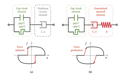
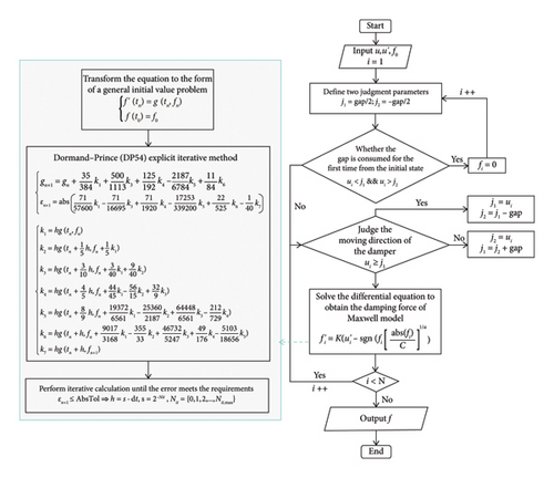
Figure 2 demonstrates the calculation procedure of the G-M model. Two judgment factors j1 and j2 are defined to determine the operational state of the damper. Regardless of the initial position of the piston head, it must always be ensured that the absolute difference between j1 and j2 equals the gap length, and the ratio of j1 and j2 corresponds to the volume ratio of air in the chambers on either side, which depends on the position of the piston head. Assuming that the damper piston is initially placed in the middle of the chamber, that is, the damper will not generate force when its movement is within the range [−gap/2, gap/2]. Therefore, the initial values of j1 and j2 are −gap/2 and gap/2, respectively. Once the damper displacement exceeds the gap for the first time, the value of the judgment parameters will change with the real-time displacement. When the damper displacement keeps increasing in the positive position, j1 will be set as ui and j2 is j1-gap. On the contrary, when the damper displacement keeps increasing in the opposing position, j2 will be set as ui and j1 is j2 + gap. The aim is to prepare for the determination of the following operational state. When the damper is within the gap, its output force is zero. When the damper displacement exceeds the gap, the damping force can be obtained by numerically solving the differential equation of the Maxwell model, in which the Dormand–Prince (DP54) explicit iterative method is employed [27]. Compared with the traditional Runge–Kutta method, the DP54 method can achieve more accurate solutions with smaller time steps.
2.2. Verification of the G-M Model
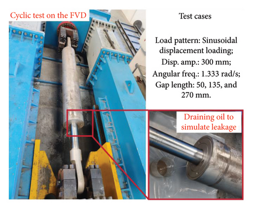
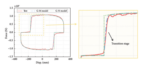
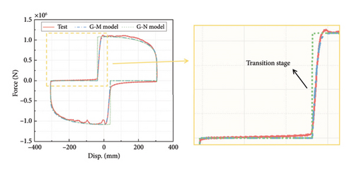
The cyclic tests conducted by Hu et al. are considered in this study to verify the feasibility of the proposed G-M model [19]. Figure 3 shows the FVD during the test and the primary test cases. The leakage was achieved by discharging oil with a given volume through the damper draining hole. Three leakage degrees were adopted, with gap lengths of 50, 135, and 270 mm, respectively. Sinusoidal displacement loading with a displacement amplitude of 300 mm and an angular frequency of 1.333 rad/s was applied in the test. The mechanical parameters of the Maxwell model, including C, α, and K, are identified based on the experimental hysteresis results of the intact FVD. These parameters are determined as 1475 kN·(s/m)α, 0.348, and 65,093 kN/m, respectively. C and α of the G-N model are 1428 kN·(s/m)α and 0.321, according to Hu et al. [16]. The comparison among the hysteresis results obtained from the experiment, the G-M model, and the G-N model is presented in Figure 4. It can be seen that both the G-M model and the G-N model have a good agreement with the test results in the zero-force state and the normal-force state. However, during the transition state, the G-M model demonstrates significantly higher accuracy and effectively captures the stiffness effect of the gradual change in damping force. The results indicate the rationality of the G-M model.

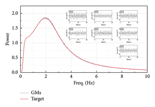
2.3. Influence of the Damper Performance Change on the Seismic Mitigation Capacity
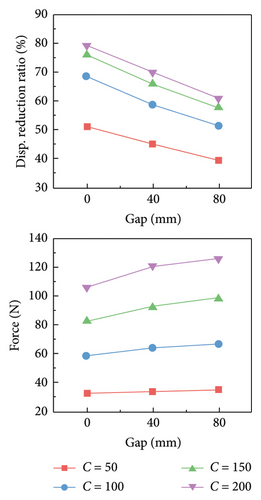
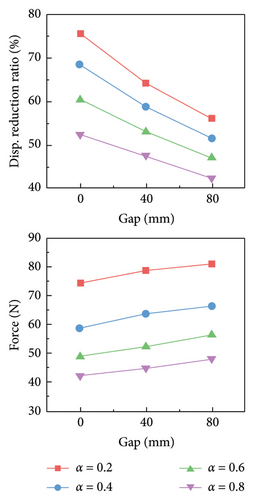
The seismic-induced peak displacement reduction ratio and maximum output force of the FVD are calculated for each set of parameters, and the results are shown in Figure 6. It can be seen that given a constant gap length, the displacement reduction ratio and output force of the FVD are positively proportional to the damping coefficient and inversely proportional to the velocity exponent. The contribution of C on the seismic performance of the damper is larger than that of α, while the stiffness has a minimal impact. Therefore, if an increase in C or a decrease in α occurs, although this is beneficial for structural protection, the damper is more likely to exceed its design capacity and suffer damage. Conversely, if a decrease in C or an increase in α occurs, although the safety of the damper is ensured, the weakened protective effectiveness may lead to structural damage. With fixed parameters, the displacement reduction ratio is negatively related to the gap length, while the output force is exactly the opposite. This is because the weakened damper will lead to a more significant structural response. Note that the FVD is velocity-dependent, a higher velocity will result in a larger damping force. This indicates that leakage in the damper is detrimental to both the damper and the structure. Therefore, regularly monitoring and assessing the operational status of the FVD is necessary to facilitate timely maintenance and replacement, ensuring its optimal performance during potential earthquakes.

3. Force Pattern of the FVD in the Railway Suspension Bridge
3.1. Simplified Longitudinal Movement Pattern of the Railway Suspension Bridge
The routine movement data of long-span bridges gathered by structural monitoring systems can be used for damper abnormality detection. The longitudinal displacement of the railway suspension bridge in the operational state is mainly affected by temperature variation, train passage loads, train braking forces, and wind loads [28]. Among these four loads, temperature variation and train passage loads typically exhibit periodic patterns and cause significant girder longitudinal displacement [29, 30]. Wind loads are usually irregular and cause smaller random displacements of the main girder [28, 31]. Train braking forces occur much less frequently than the other three load types [32]. Therefore, temperature variations and train passage loads can be considered the primary contributors to the girder longitudinal displacement, and displacements caused by wind loads and train braking forces can be regarded as noise.
Note that the girder displacement approximately adopts a linear correlation with the temperature [9, 33]. Assuming that the temperature follows a sinusoidal trend throughout the day, the temperature-induced displacement can be simulated by a one-cycle sinusoidal wave with a very low frequency [34]. Similarly, Liang et al. [35] and Wang et al. [36] revealed that the passage load will also lead to sinusoidal oscillation of the suspension bridge girder. Hence, the displacement caused by train passage in a day can be represented by several periods of sinusoidal waves with relatively high frequency. Considering the intervals between consecutive train operations, a window period is included in each cycle. Therefore, the simplified longitudinal girder displacement and velocity modes of the railway suspension bridge are determined and shown in Figure 7.
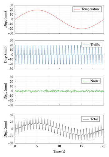
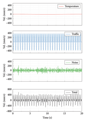
Due to the significant computational effort required for calculation over a 24-h cycle, this study only adopts a similar motion pattern without considering the actual duration, amplitude, and frequency. For computational convenience, the peak of temperature-induced displacement is set to 20 mm with an angular frequency of π/10; the peak of train-induced displacement is set to 20 mm with an angular frequency of 6π; and the noise amplitude is set to 5 mm with an upper angular frequency limit of 12π. The total duration is 20 s, and the window length between consecutive train operations is equal to the period of the train-induced displacement. In subsequent calculations, the displacements caused by temperature and train remain constant, while the noise is generated randomly each time to ensure the credibility of the calculation results.
3.2. Force Pattern of the FVD
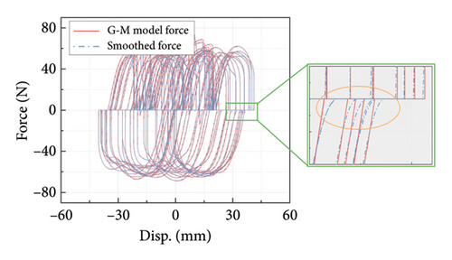
The damping force time history and hysteresis curve of the leaked FVD due to the displacement loading as shown in Figure 7(a) can be determined and presented in Figure 8. Compared with the damping force of the Maxwell model without oil leakage, there is an apparent zero-output stage in the time history of the force produced by the G-M model, as shown in Figure 8(a), indicating that the damper does not overcome the gap at this time. A similar phenomenon can also be observed in the hysteresis curve in Figure 8(b), in which the zero-force platforms appear at every change in the moving direction. The hysteresis curve is cluttered under the influence of gap and noise, so they cannot be directly analyzed by traditional parameter identification methods. Therefore, a condition identification procedure is proposed in the following sections to determine the gap length and the parameter change of the FVD under such a situation. Note that the damper force in the experiment changes smoothly following the overcome of the gap, as shown in Figure 4, which impacts the gap identification. To better reflect the reality and enhance the practicality of the proposed gap identification method, the original damping force data were smoothed during the subsequent gap identification process, as shown in Figure 8(b).

4. The SGI Method
4.1. The Gap Identification Procedure
It can be seen from Figure 4 that the damping force within the gap exhibits a minimal value rather than zero, indicating that obtaining the gap length simply by determining the length of zero-force parts is impractical in engineering applications. A practical approach is to define damping forces smaller than a certain threshold as the output within the gap, and the threshold can be set at a proportion of the maximum damping force. This method can be called the overall gap identification (OGI) method and is applicable for single-cycle data with minimal noise. However, as illustrated in Figure 8, under multicycle motion with superimposed noise, the peak damping force varies in each cycle. Using the maximum damping force throughout the whole dataset would significantly overestimate the gap length. Therefore, the SGI method is proposed.
The main idea of the SGI method is to divide the entire dataset into N segments, calculate the maximum force, and obtain the gap length for each segment. The number of segments is determined by the number of cycles in the damping force time history. In this study, it is recommended that each segment contains 2 to 3 cycles. A smaller number of cycles may lead to the division of gap lengths, while a larger number of cycles might include some small-amplitude cyclic motions as gaps. The damping force time history used in this study can be approximately divided into 30 cycles; thereby, N is set to 10. The final gap length is derived by averaging the gap lengths of all segments. The implementation process is shown in Figure 9.

4.2. Verification of the SGI Method
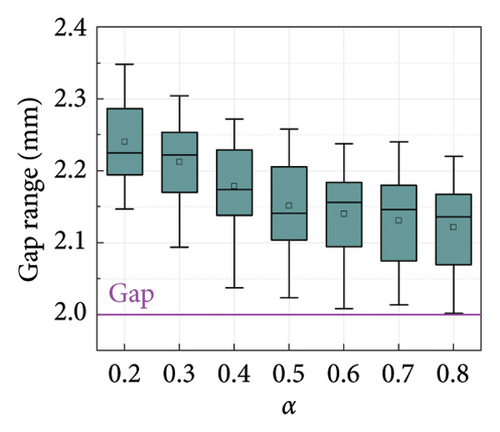
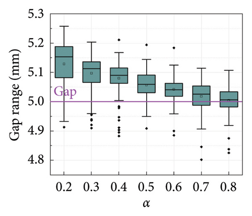
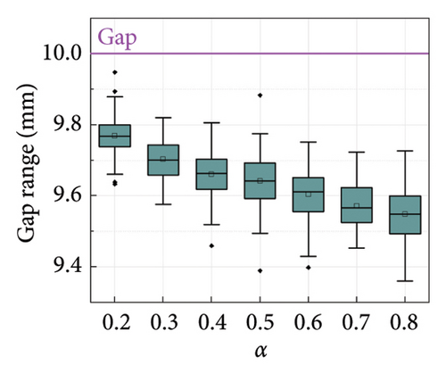
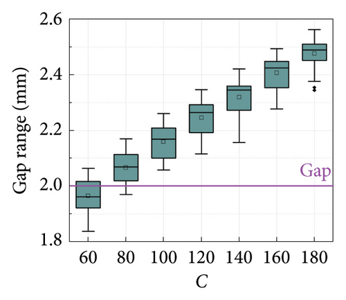
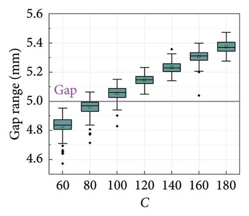
Since the feasibility of the G-M model has been demonstrated in Section 2, numerical simulations based on the G-M model are performed in this section to verify the accuracy of the SGI method. Table 1 lists the calculation cases. Different damping coefficients C and velocity exponents α are considered to investigate the adaptability of the SGI method to various damper parameters. Given the nonlinear damper parameters commonly used in civil engineering [4, 5], the range of velocity exponents in this simulation is set to [0.2, 0.8], thereby making the numerical conclusions more reflective of practical scenarios. Three gap lengths are selected to reflect different leakage severities, that is, 2, 5, and 10 mm. The threshold for evaluating the gap length is set to 5% of the maximum force of each segment. To account for the impact of the noise randomness, each set of damper parameters is computed 100 times, with noise being randomly generated anew for each calculation, thus ensuring the generalizability of the overall results.
| Case | Parameters of the Maxwell element | Parameters of the gap element | ||
|---|---|---|---|---|
| C [N·(s/m)α] | α | K (N/m) | Gap length (mm) | |
| α change | 100 | 0.2–0.8 | 10,000 | 2, 5, 10 |
| C change | 60–180 | 0.5 | 10,000 | 2, 5, 10 |
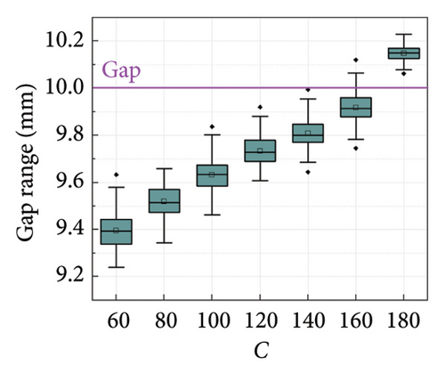
The box plots of the gap identification results under different cases are shown in Figures 10 and 11. It can be seen that the error in the average value of the gap identification results is within 10% for most cases, indicating a high accuracy of the proposed SGI method. The robustness of the SGI method can also be proved by the compact distribution of the calculation results. However, it is worth noting that the identification error for small gap cases is greater than that for large gap cases. The maximum error occurs in the case of C = 180, with an error close to 25%, as shown in Figure 11(a). This can be attributed to the identification of smaller gaps being more vulnerable to the selected threshold and noise. Considering that small gaps have a limited impact on the damper performance, these identification results are still acceptable for engineering applications.
4.3. Comparison Between the SGI Method and the OGI Method
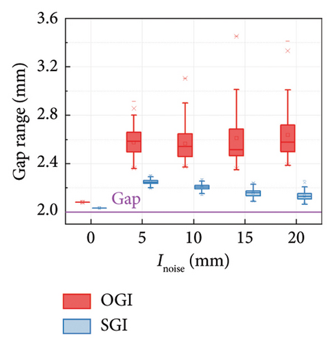
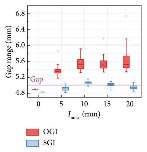
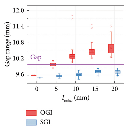
A comparison between the results obtained by the SGI method and the OGI method is further performed to show the superiority of the SGI method. The damper parameters are set as C = 100 N·(s/m)α, α = 0.5, and K = 10,000 N/m. Five noise intensities (Inoise) are considered, that is, 0, 5, 10, 15, and 20 mm. The comparison results are presented in Figure 12. It can be seen that the calculation results of both methods are reliable in noise-free cases. However, as the noise intensity grows, the error in the results obtained by the OGI method increases, and the uncertainty of the results is significant. In contrast, the accuracy of the SGI method remains relatively unaffected by changes in noise intensity. The results indicate that the SGI method outperforms the OGI method in terms of both accuracy and robustness.
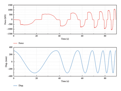
Additionally, the cyclic test results obtained by Hu et al. [19] are adopted to further verify the superiority of the SGI method. The tested FVD exhibits a gap with a length of 140 mm. Displacement loading is applied, with a constant amplitude of 300 mm and an increasing frequency from 0.167 to 1.333 rad/s. The loading lasted a total of six cycles. The time histories of the damping force and the displacement are shown in Figure 13. It can be seen that the maximum force in each segment is increasing. The peak force in the last segment is nearly twice of that in the first segment. Two and three segments are, respectively, considered in the SGI method. Table 2 lists the identification results of the gap length in each segment obtained by the SGI method and compares the average value derived by the SGI method and the OGI method.
| Method | Gap length (mm) | ||||
|---|---|---|---|---|---|
| Seg. 1 | Seg. 2 | Seg. 3 | Average | ||
| SGI | 2 Segments | 139.23 | 125.35 | / | 132.29 |
| 3 Segments | 134.54 | 128.61 | 124.16 | 129.10 | |
| OGI | / | / | / | 160.43 | |
| Test | 140 | 140 | 140 | 140 | |
It can be seen that the gap length obtained by the SGI method is closer to the designed value, while the OGI method leads to an overestimation. This is because when the damping force varies significantly throughout the entire loading process, the OGI method uses the maximum value across the process as the reference criterion. As a result, some phases with relatively low output are mistakenly identified as gaps, leading to an overestimation of the gap size. In contrast, the SGI method divides the entire dataset into several smaller subsets, allowing the maximum force in each segment to be used as the reference criterion. This approach reduces the impact of variations in peak force. Therefore, the SGI method can lead to a more reasonable result.
5. The GMPI Method
5.1. The Overall Procedure
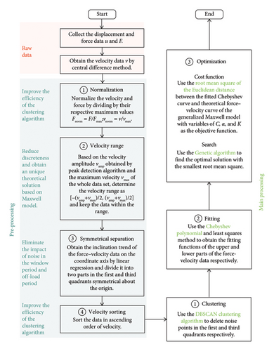
Figure 14 shows the overall procedure of the GMPI method. Three main parts are included in this method, that is, gathering raw data, preprocessing, and main processing. First, the raw data are artificially generated following the displacement and force modes as described in Section 2. The central difference method is applied to the displacement time history to get the velocity time series data. Second, four preprocessing steps are employed, that is, normalization, determination of velocity range, symmetrical separation, and sorting based on velocity. The aim is to reduce the discreteness caused by noise and enhance the efficiency of the subsequent clustering. Detailed methods are introduced in Section 5.2. Finally, three main processing steps should be followed to obtain the final identified parameters, including clustering, fitting, and optimization. The DBSCAN algorithm is applied to retain meaningful force–velocity data. The CPF algorithm is used to obtain nonparametric force–velocity characteristics. The GA is employed to find the best-fitting damper parameters. Detailed methods are introduced in the Appendix.
5.2. Verification of the Parameter Identification Method
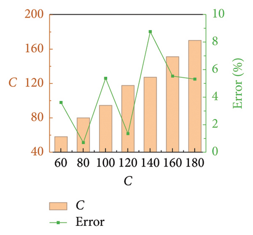
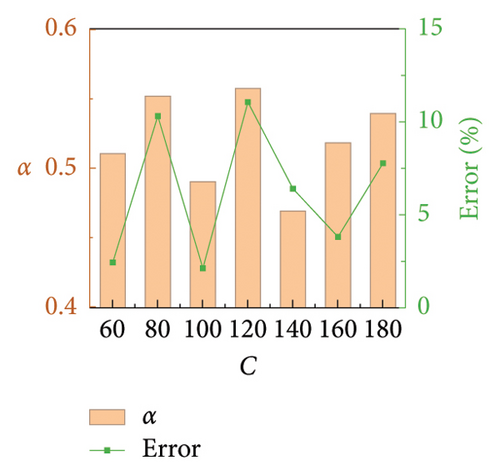
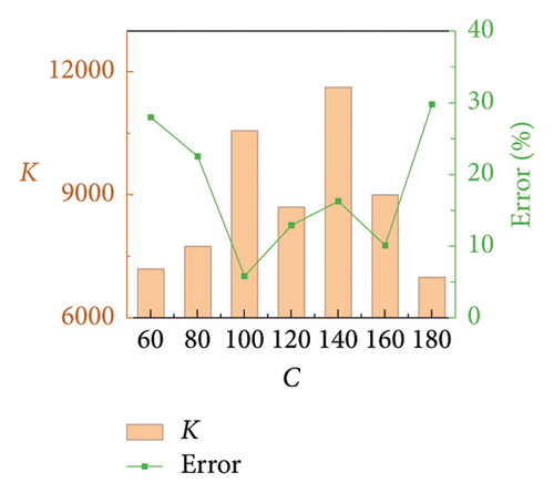
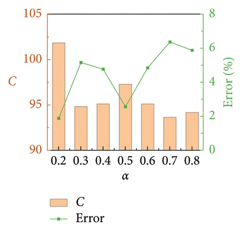
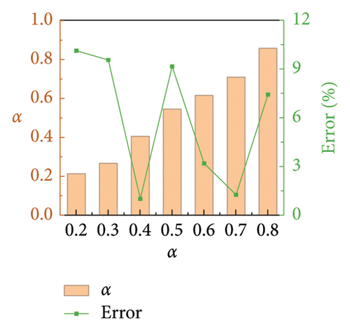
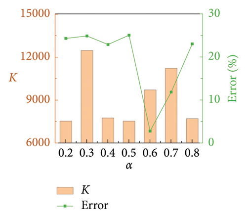
Numerical simulations are conducted to validate the proposed parameter identification method for FVDs in railway suspension bridges. Similar to Section 2.3, baseline damper parameters are determined as C = 100 N·(s/m)α, α = 0.5, and K = 10,000 N/m. Only one parameter changes at a time. Same as Section 4.2, C varies from 60 to 180 with an interval of 20 and α from 0.2 to 0.8 with an interval of 0.1, while K is a constant. The identification results are shown in Figures 15 and 16. It can be seen that the errors in the identification results of C and α are less than 9% and 12%, respectively. The obtained C tends to be slightly lower than the theoretical value, while α oscillates around the theoretical value. However, accurately capturing the value of K seems to be more challenging, with a maximum error approaching 30%. As demonstrated in Section 2.3, C and α have the most significant impact on the dynamic performance of the FVD, while the contribution of K can be ignored when its value is dozens of times greater than that of C. Therefore, the accuracy of the proposed FVD parameter identification method should be acceptable for engineering applications.
6. Conclusion
- 1.
The G-M model comprises a gap–hook element group and a Maxwell element connected in series. The oil leakage is simulated by assigning different gap lengths, and the change in damping performance can be achieved by altering the mechanical parameters. Compared with the G-N viscous model, the G-M model is more accurate in reproducing the dynamic stiffness phenomenon at the transition stage when the gap is consumed and the damper starts to generate force.
- 2.
Regarding parameter changes in the FVD, an increase in C or a decrease in α means a higher risk of force-exceeding failure. In contrast, a decrease in C or an increase in α indicates a worse vibration control capacity. For the FVD suffering from oil leakage, a less effective displacement mitigation ratio is obtained with a higher damper output, which is disadvantageous to both the damper and the structure. Therefore, monitoring and identifying the damper performance change is necessary to ensure timely maintenance.
- 3.
The proposed SGI method reduces the impact of noise by dividing the original data into several segments, calculating the damping force threshold and identifying gaps in each segment separately. Numerical results indicate that the SGI method can accurately assess the gap length of dampers with varying parameters and noise pollution. Compared with the OGI method, the SGI method exhibits greater robustness under noisy conditions.
- 4.
The GMPI method follows a procedure of preprocessing, clustering, fitting, and optimization to achieve parametric identification of the damping coefficient, velocity exponent, and dynamic stiffness in the G-M model. Numerical results indicate that this method has high accuracy in identifying the damping coefficient and velocity exponent, but the detection error for stiffness is relatively large. However, considering that the stiffness has a negligible effect on damper performance when large enough, the identification accuracy is acceptable for engineering applications.
Note that the condition detection method in this study is based on the simplified longitudinal moving pattern of the railway suspension bridge girder under the operational condition, more studies are needed when other types of bridges or loads are considered to examine its applicability.
Conflicts of Interest
The authors declare no conflicts of interest.
Funding
This research was funded by the China National Postdoctoral Program for Innovative Talents (No. BX20230429); the China Postdoctoral Science Foundation (No. 2023M733970, 2024M750618); and the Postdoctoral Fellowship Program of CPSF (No. GZC20240325).
Appendix
This appendix provides the detailed calculation process and supporting figures for the analysis presented in Section 5 of the paper. The calculations outline the steps used to derive the key results, while the figures illustrate specific examples discussed in the main text.
Appendix A: The Preprocessing of the GMPI Method
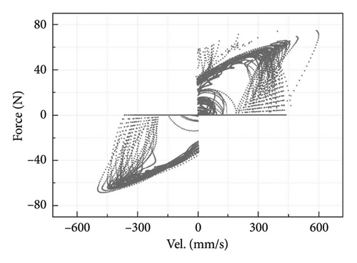
An example of the raw force-velocity data of the G-M model is presented in Figure A1(a), which is calculated based on the displacement loading in Figure 7. Under the coupling effect of gap and noise, the force–velocity data exhibit three peculiarities: (i) the data only exist in the first and third quadrants. The force that should originally exist in the second and fourth quadrants, representing data during reverse loading, becomes zero due to the presence of gaps; (ii) the data during the unloading phase appear scattered because noise influencing the velocity peaks during each cycle; (iii) the force-velocity data still in general exhibit a trend of symmetry about the origin in overall due to the symmetry of the train passage induced velocity. Therefore, several pre-processing should be performed to improve the operability of the data.
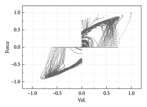
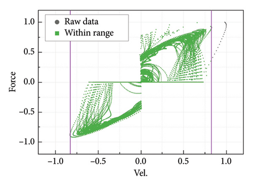
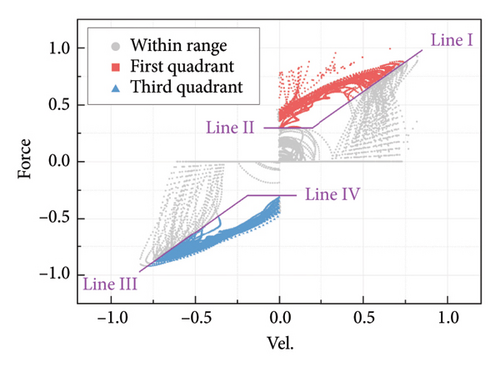
The third step is to separate the force-velocity data symmetrically. Since the data in the first and third quadrants have different fitting functions, they must be considered respectively. Another target of the separation is to eliminate the impact of noise in the unloading phase and during the window period. Therefore, the data in each quadrant are separated by two lines, as shown in Figure A2(b). The data in the first quadrant are taken as an example. Line I is used to delete the data in the unloading phase. Its slope is derived by conducting linear fitting on the whole dataset. Line II is used to delete the noise during the window period. Similarly, lines III and IV are applied to retain meaningful data in the third quadrant. The fourth step is to sort the data in ascending order of velocity, which can improve the efficiency of the clustering algorithm.
Appendix B: The Main Processing of the GMPI Method
- (i)
Giving two core parameters ε and MinPts.
- (ii)
A point is a core point pc if there are at least MinPts points q (including pc) within a distance ε from it, that is,
(B.1) - (iii)
A point is a directly density-reachable point if p is a core point and q is within distance ε of p, that is,
(B.2) - (iv)
A point is a density-reachable point if there is a chain of points p1, p2, …, pn where pi = p and pn = q, and each pi+1 is directly density-reachable from pi.
- (v)
Two points are density-connected if there is a point o such that both p and q are density-reachable from o.
- (vi)
Points not density-reachable from any other point are regarded as noise.
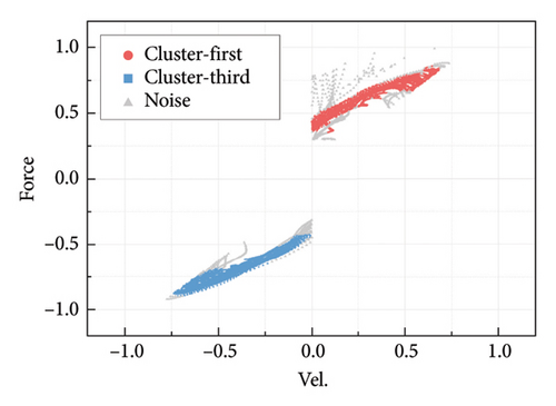
The clustering result based on the data in Figure A2(b) is presented in Figure A3(a). It can be seen that some of the divergence data have been cleared up, which can enhance the fitting accuracy of the subsequent step.
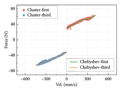
Since the data in the first and third quadrants may yield different fitting functions, they are calculated separately. The fitting result in Figure A3(b) indicates that the fitted functions in both the first and third quadrants can accurately represent the values and trends of the force-velocity relationship of the damper.
Optimization. Reflecting the performance changes of the FVD in its direct parameter variations allows engineers to make more intuitive judgments, facilitating the maintenance and replacement of the damper. The Chebyshev polynomial derived above can be compared with the theoretical force–velocity curves under different parameters to obtain the most accurate damper parameters. The parameters with the slightest deviation are considered the optimal solution. The theoretical force–velocity curves are determined by applying sinusoidal loading to the ideal generalized Maxwell model, with the frequency and amplitude of the loading calculated using the method proposed in Appendix A. The cost function is defined as the root mean square of the Euclidean distance between the fitted polynomial and the theoretical force–velocity curve within the velocity range defined in Appendix A, and the optimization is performed using the GA [40].
Open Research
Data Availability Statement
Some or all data, models, or codes that support the findings of this study are available from the corresponding author upon reasonable request.


