Summary

1. Introduction

Over the past few years, there has been a significant increase in the demand for motion planning of robots and automated transportation vehicles in obstacle-crowded environments. Motion planning algorithms have become essential for enabling mobile robots to navigate and operate efficiently in unpredictable and obstacle-crowded scenarios. Mobile robots have been deployed in various sectors, such as healthcare, logistics, delivery services, tourism, and more [1–3].

Probabilistic roadmap (PRM) has gained considerable popularity as motion planning techniques [4, 5]. PRM is a motion planning algorithm that computes a roadmap by randomly sampling the planner for obstacle-free location points. Then, for each point, the algorithm connects it with several close neighbors if they are close enough and there are no obstacles in between [6]. Typically, two predefined points representing the start and target of the trajectory are added before generating random location points. The resultant structure forms a weighted graph. To determine the optimal trajectory between the start and target, a sub-algorithm like Dijkstra’s or A^∗ is integrated after the construction of the roadmap. Detailed information and pseudocode for the PRM algorithm can be found in Kavraki et al. and Choset et al. [6, 7].

This paper is structured as follows: Section I serves as the introduction, setting the stage for the research. In Section II, a review of related work is provided, describing various enhancement algorithms of PRM. In Sections III and IV, our proposed algorithms, R-PRM and TR-PRM, are presented. The simulation and experimental results are demonstrated in Section V. Finally, Section VI concludes this paper.

2. Related Work

There are numerous approaches and diverse methods available for managing obstacles. Rafai, Adzhar, and Jatini [8] provided an extensive overview of these methods. Within this article, we aim to extend their discussion in the subsection dedicated to PRM and motion planning algorithms.

Since PRM does not guarantee optimal solutions, numerous researchers have suggested diverse modifications to enhance the path length and the runtime of the algorithms. These modifications aim to reduce computational complexity and increase the accuracy of the results. Some proposed approaches include implementing heuristics, adjusting sampling strategies, and incorporating machine learning techniques to predict optimal paths. Moreover, researchers have been exploring the combination of multiple algorithms and developing hybrid algorithms to leverage the strengths of different methods for improved performance [9]. In this section, we review several modifications that have been suggested as enhancements to the conventional algorithm.

Bohlin and Kavraki [10] introduced Lazy-PRM, an algorithm that constructs a roadmap without relying on collision detection, initially assuming all edges are collision-free. During query execution, an A^∗ search is used, and any detected collisions lead to the removal and rechecking of edges until a collision-free path is found. Lazy-PRM is more efficient than PRM in maps with fewer obstacles but requires more memory due to increased connectivity. The primary difference between the two lies in execution time.

Boor, Overmars, and Van Der Stappen [11] introduced Gaussian PRM, which adds valid configurations to the roadmap at a specified fixed distance from obstacles. Gaussian sampling can be computationally intensive due to the complexity of finding configurations that meet the distance condition, as well as the selection of the right fixed distance. A small distance may generate configurations too close to obstacles, while a large distance may miss critical areas. Additionally, this approach may overlook connectivity in obstacle-free regions, potentially leading to suboptimal solutions.

Denny and Amato [12] introduced Toggle PRM which constructs dual roadmaps in both the configuration and obstacle spaces. The approach coordinates the roadmap construction, using failed connections in one space to enhance the other. This strategy improves the efficiency of mapping narrow spaces. However, maintaining a large number of effective sampling points in both spaces poses challenges, including significant time and storage demands.

Amato et al. [13] introduced the obstacle-based PRM (OBPRM) algorithm, which generates nodes close to obstacle surfaces. The process starts with an initial invalid point, c_in, on an obstacle. A random ray extends from c_in to find a clear node, c_out, and a bisection search is used to iteratively move from c_in to c_out until a boundary point is found. These boundary points are retained as nodes in the roadmap. Like Gaussian PRM, OBPRM faces similar challenges, along with significantly longer running times.

Lien, Thomas, and Amato [14] introduced medial axis PRM (MAPRM), which pushes sample nodes (valid and invalid) toward the medial axis of the configuration-free space, ensuring paths with greater obstacle clearance for safer navigation. This method improves sampling probability in narrow passages compared to uniform random sampling. However, it remains computationally intensive, even with approximations.

Ye, Chen, and Zhou [15] introduced obstacle potential field probabilistic path map (OP-PRM), which enhances pathfinding by focusing sampling around obstacles using a potential field approach and then applies the D^∗ Lite algorithm for efficient path searching in complex environments. This method can improve navigation in dynamic and cluttered spaces, offering a responsive solution to real-time path planning.

Faust et al. [16] introduced PRM reinforcement learning (PRM-RL), which integrates reinforcement learning with PRM to build a connectivity-aware roadmap for long-range robotic navigation tasks. The method combines RL to optimize navigation policies for robot dynamics and task constraints with PRM to create a roadmap that adapts to large, complex environments. PRM-RL enhances pathfinding by learning short-range navigation policies, while the PRM provides global connectivity, improving efficiency in dynamic settings.

Ravankar et al. [17] introduced the hybrid potential-based PRM (HPPRM), which combines PRM with artificial potential fields to improve dynamic path planning for mobile robots. This hybrid approach enhances adaptability in narrow passages and environments with both static and dynamic obstacles, leveraging PRM’s global connectivity and potential fields’ local obstacle avoidance.

Mohanta and Keshari [18] introduced a knowledge-based fuzzy-PRM (Fuzzy-PRM) method for mobile robot navigation, which integrates fuzzy logic with PRMs to enhance path planning in uncertain environments. This approach improves adaptability in complex scenarios, including narrow passages and environments with both static and dynamic obstacles, by combining the global connectivity of PRMs with the local decision-making capabilities of fuzzy logic.

Ma et al. [19] introduced improved PRM based on cubic spline (CSb-PRM), which combines bidirectional search with cubic spline interpolation to enhance path planning. This method reduces unnecessary node connections and improves path smoothness, resulting in more efficient and safer navigation in complex environments.

While each algorithm serves a specific purpose and offers unique advantages, none focuses on significantly reducing running time, memory usage, or optimizing computation in specific areas. These algorithms uniformly cover the entire map, lacking targeted efficiency improvements. Additionally, most of them are not incremental; if the environment changes during the robot’s movement, the entire map must be recalculated. Some algorithms add additional processes to PRM, either before or after its execution. While these approaches can improve the final path, they tend to be computationally expensive, especially in large, obstacle-crowded environments. In this article, we demonstrate that as the complexity of the problem increases, our algorithm’s computational load grows more efficiently compared to existing methods. Therefore, we compare our approach with similar algorithms that modify the PRM algorithm, either by adjusting node distribution or altering the search strategy.

3. R-PRM

In this section, we describe the motivation and algorithmic components of R-PRM, which is an enhanced version of the PRM algorithm, featuring built-in computational capability that obviates the necessity for Dijkstra or A^∗ algorithms to find a path. The intelligent capabilities of R-PRM enable it to efficiently navigate the configuration space and discover feasible paths independently.

The motivation for R-PRM lies heavily in the observation that PRM often performs calculations in unreachable areas. This occurs due to PRM’s construction of unnecessary edges in regions that are blocked. Such redundant computations not only add to the computational workload but also hinder the efficiency of the path planning process. R-PRM overcomes this disadvantage by incrementally constructing a graph in a breadth-first search (BFS) manner. Rather than connecting neighbors in a distributed way, the graph is built progressively from the starting node and extends exclusively to its immediate neighbors. The expansion continues from the nearest neighbor to the target. With this method, the algorithm expands only to accessible areas and bypasses blocked areas that cannot be reached. Another advantage arising from this method is that the algorithm can maintain a previous link for each node, which eventually allows it to find a reasonable trajectory from s to t (if it exists) using backtracking.

Algorithmically, R-PRM is an enhanced modification of PRM, with the primary change occurring in the second stage of the algorithm, specifically in how the edges between the nodes are assigned. While PRM traverses the nodes in the order allocated on the map, R-PRM operates differently by only allowing transitions between the nodes connected during the expansion process. This transition process shares similarities with the BFS method [20] while also incorporating distinct motifs from the Dijkstra’s shortest path algorithm [20]. It commences from the starting node, connects its k nearest neighbors, and inserts them into a queue. The algorithm then continues the expansion by extracting neighbors from the queue and further exploring their neighbors until the queue is empty. Throughout this process, R-PRM keeps track of the previous node for each configuration and its distance from the start, facilitating the identification of a reasonable trajectory from the start to the target.

The steps of the R-PRM algorithm are summarized as follows:

3.3. Step 3: Retrieve Path, Lines 48–52

After visiting all reachable nodes starting from s, the algorithm checks whether node t was also visited. If t was not visited, there is no valid path to it from s, and NIL is returned. Otherwise, backtracking is used to retrieve the path.

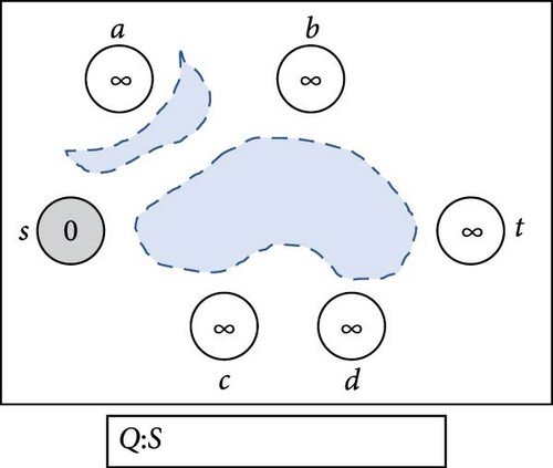
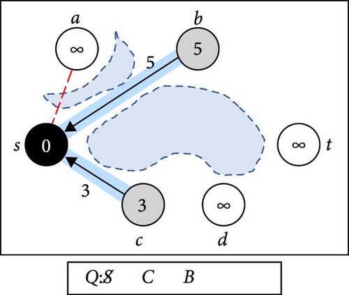
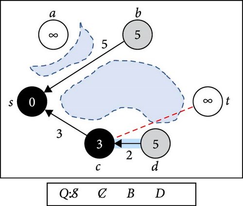
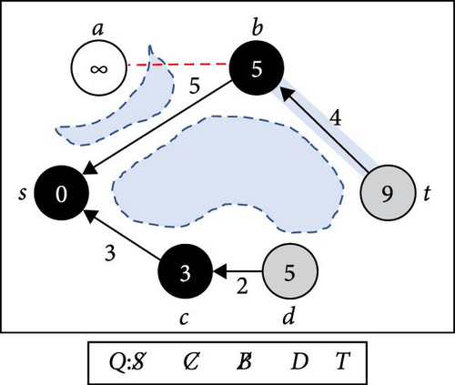
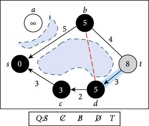
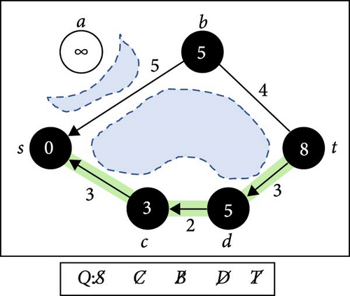
Figure 1 shows the execution of Algorithm 1 after the nodes have been placed on a plain map with six obstacles of different sizes. Underneath each diagram, there is a queue that represents the progress status.

Algorithm 1: R-PRM.

• Inputs: s: Start node, t: Target node, n: Max nodes, k: Near neighbors, M: map

• Output: A path from the start node s to the goal node g

•  1. G(V, E) ← New Graph( )

•  2. if (!(s, t are valid points and are collision free in M)) then

•  3.  return NIL

•  4. end if

•  5. V ← V ∪ {s, parent : 0, visited : true, interval : 0}

•  6. V ← V ∪ {t, parent : −1, visited : falsex, intervalx : ∞}

•  7. while (|V| < n) do

•  8.   do

•  9.    u ← a random configuration in M

•  10.  until (u is a valid point and is collision  free in M)

•  11.  V ← V ∪ {u, parent : −1, visited :  false, interval : ∞}

•  12. end while

•  13. Q ← New Queue (size : n)

•  14. Enqueue (Q, s)

•  15. while (not_empty (Q)) do

•  16.  u ← Dequeue (Q)

•  17.  PQ ← New Priority Queue (size : k, type : max)

•  18.  fill PQ with k configurations with priority  = ∞

•  19.  foreach (node v ∈ V)

•  20.   if(v = u) then

•  21.     continue

•  22.   end if

•  23.   e ← Cast a stright ray in M between (u, v)

•  24.   if(e_dist < front (PQ).priority) then

•  25.    Dequeue (PQ)

•  26.    Enqueue (PQ, e, e_dist)

•  27.   end if

•  28.  end foreach

•  29.  while (not_empty (PQ)) do

•  30.   e, v ← dequeue (PQ)

•  31.   if(e_cross = 0) then

•  32.      if(e ∉ E) then

•  33.       E ← E ∪ {e}

•  34.      end if

•  35.      if (v.visited  = false ) then

•  36.       v ← set : {visited : true, parent : u, interval : u.interval  + e_dist}

•  37.       Enqueue (Q, v)

•  38.      else

•  39.       if (v.interval  > u.interval  + e_dist) then

•  40.         v ← set : {parent  = u, interval  : u.interval  + e_dist}

•  41.       else if (u.interval  > v.interval  + e_dist) then

•  42.         u ← set : {parent  = v, interval  : v.interval  + e_dist}

•  43.       end if

•  44.      end if

•  45.     end if

•  46.   end while

•  47. end while

•  48. if (t.visited  = true) then

•  49.   Path ← BackTracking (G, t)

•  50.   return Path

•  51. end if

•  52. return NIL

In Figure 1, we set the start node to be S and the target node to be T. Unvisited nodes are marked in white, and visited nodes are marked gray. Dequeued nodes are marked in black, and each visited node has a single arrow marking its parent. In (a), the initialize step, the starting node S is enqueued to Q, marked as visited with a distance of 0, while all other nodes are marked unvisited with a distance of ∞. In (b), S is dequeued and connected to the nearest neighbors C and B. Node A is unreachable from S, so it is skipped. C and B are enqueued to Q according to their distance from S, marked as visited with proper distance, and S is set as their parent. At (c), C is dequeued and expanded to D, setting C as its parent, and the distance to D represents the total distance from S passing through C. In (d), node B is dequeued, and B connects to node T. Although the target is achieved, the expansion continues in case of an improved trajectory. In (e), the graph expands to node T from D, which has already been visited from B. The distance to T from D is better than that from B to T, so T’s parent is updated to D. At step (f), T is dequeued, and since there are no more nodes in Q, and node T is marked as visited, a valid path is obtained through backtracking.

Unlike the combination of PRM with A^∗, the R-PRM algorithm does not rely on heuristic assumptions while calculating the final route, leading to a higher probability of obtaining more accurate solutions. However, it may encounter challenges in terms of speed and target orientation. The objective of the algorithm in the next section is to overcome these limitations and further improve its performance.

4. TR-PRM

These drawbacks collectively pose significant challenges for these algorithms in scenarios involving expansive maps replete with obstacles. This compounded effect noticeably impacts various facets including running time, memory utilization, node count in the final route, and its overall length. As the problem complexity escalates, these challenges intensify, leading to notable increases across these critical parameters.

In addition, all the previously presented algorithms are nongradual; they calculate everything in advance and are unable to consider the possibility of dynamic changes in the environment. Consequently, they are not well-suited to work in dynamic areas, such as hospitals, where obstacle locations may change while the robot is in motion, so calculations made further down the road may no longer be relevant.

We can minimize the disadvantages of the previous algorithms in most cases where it is known in advance where our target destination is, and the obstacles located on the map are not arranged in a way that creates a maze. This can be achieved by examining several possible directions from the starting node to predefined target area and dealing individually in real time with obstacles encountered along the way.

The proposed algorithm offers an efficient pathfinding method through an obstacle-laden map. Its core idea involves exploring several random directions from the starting node to the target area. This “target area” is better described as an adaptable space rather than a specific node on the map. It represents a zone in proximity to the desired target node, allowing for a range of acceptable endpoints that facilitate successful pathfinding within the map. Each landmark inside the zone is both near the desired target and obstacle-free along a direct line to the target node. The algorithm’s objective is to reach any location within this target area. The rationale behind exploring multiple directions is as follows: comparing several routes helps in avoiding potential directions that are too crowded. By selecting the path with as few obstacles as possible, it minimizes the need for frequent maneuvers and results in a smoother final path.

To achieve this, we place m random nodes in the target area and draw direct lines from each of these nodes to the starting point, creating a type of ray casting from the start to the target. If any of these rays do not intersect with any obstacles, we can add it as an edge to the exploring roadmap and calculate the final trajectory. However, if a projected ray intersects with obstacles, we choose the one that crosses the fewest obstacles and follow it from the starting node until we encounter the first obstacle. At this point, we place a new node adjacent to the blocking obstacle, allowing us to find a way to maneuver around it. Here, the R-PRM algorithm comes into play, but in an altered version, where the objective is not to reach the destination directly but merely to find a detour.

In contrast to the standard approach, which involves creating randomized nodes across the entire plane, this algorithm focuses solely on the area around the blocking obstacle. It achieves this by drawing a circle with its center at the adjacent node and only allocates randomized nodes within this circle. To ensure successful maneuvering, the circle must completely surround the entire obstacle. The size of the circle should be determined by the dimensions of the largest obstacle on the map, taking into account situations where obstacles that are very closely adjacent should be considered as a single obstacle.

Since the circle’s area is relatively small, the number of nodes, the distances between them, the amount of constructed edges, and the search process are all accordingly reduced. This leads to an improved runtime when constructing the roadmap within the circle. During the roadmap’s construction, the algorithm searches for an optimal point that minimizes the distance to the target area. The construction occurs only through passages to the neighbors, guaranteeing a path from the start to the optimal point.

For reader convenience, we separate the process of prioritizing the cast rays into Algorithm 2 described below:

In Algorithm 2, for each target node t, located in the target area, we cast a ray from the starting point s. Each cast is presented as an edge with additional parameters: distance (dist) and number of obstacles crossing (cross). We insert all the edges into a minimum priority queue directed by those two parameters, where the priority is determined first by the number of obstacles crossed and second by the distance. The function returns the priority queue, which is used in Algorithm 3.

Since our objective is to find a path, Algorithm 3 always strives to move forward toward the target area. Let M be a density plain, where the starting node s ∈ M and the finishing target area T ∈ M are located inside the map. We say that getting to any point t ∈ T from s satisfies us. Let R be the final routing solution of the algorithm. Assuming the location of the target area is already known in advance, the following is a description of the algorithm divided into steps:

4.5. Step 5: Continue From the Optimal Node as the New Starting Node

The algorithm conjoins the path received from R-PRM with R and continues to expand from step 2, considering the optimal node as the new starting node.

To provide a clear understanding of the system’s workflow and the interconnections between its components, Figure 2 illustrates the complete pipeline. This visual representation includes key elements such as R-PRM, TR-PRM, and ray casting, highlighting their roles in achieving efficient path planning.

Figure 3 shows an execution of Algorithm 3 on an obstacle-laden map. The illustrations depict the algorithm’s choice of path, finding a detour around a blocking obstacle, and continuing toward the target.

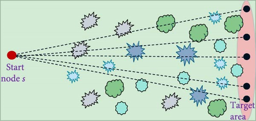
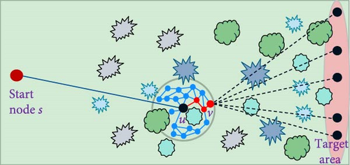
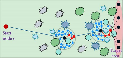
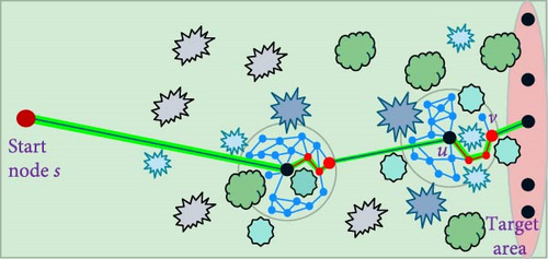
In Figure 3, the start node S is situated on the left side of the map, while the Target-Area comprises five5 target nodes on the right side. In (a), the algorithm project five rays from S to all target nodes, aiming to identify the optimal ray that encounters the fewest obstacles. Transitioning to (b), we observe the expansion of the roadmap until it reaches the first obstacle, along with the maneuvering process carried out using Algorithm 1 to navigate around it. The goal is to locate an optimal node v through a search process that minimizes the distance to any node t_i within the Target-Area. The path from u to v is then established using a backtracking approach. The algorithm proceeds from node v as the new starting point and, originating from it, projects an additional set of 5 rays to each node t_i within the Target-Area. The process at (c) replicates the procedure depicted in (b). In (d), one of the ray projections to the Target-Area does not intersect with any obstacles. Consequently, a line is drawn from the optimal node v to the relevant t_i. At this point, the algorithm concludes. The final path is derived by backtracking from t_i back to starting node S.

5. Algorithm Experiments and Real-World Simulations

In this section, we numerically and visually analyze the advantages of TR-PRM over the state-of-the-art classic PRM variant algorithms. Specifically, we compare TR-PRM with PRM its related modifications as described in the related work section. The experiments focus on the density of obstacles in combination with the density of nodes allocated on the map and were conducted on real-world and randomly generated maps. The purpose of the real-life simulations is to manage the navigation of mobile robots in various scenarios.

Simulations were implemented in a combination of C and C#, leveraging the computational efficiency of C for calculations and utilizing C#’s graphics library for visual presentation. The simulations were conducted using Visual Studio 2019 on a Windows 10 operating system with a 1.8 GHz processor and 16 GB of RAM.

All simulation environments can be considered analogous to a real-world scenario where obstacle locations are known through methods such as navigation space layout, image processing, or high-range sensor applications. The robot, starting from an initial position, is aware of its target position and the obstacle information.

We evaluated the efficacy of TR-PRM against various algorithmic versions of PRM, drawing from the following sources: PRM from [7], Lazy-PRM [10], Gaussian PRM [11], and HPPRM [17]. All methods use the Euclidean distance metric and a straight-line local planner in k nearest neighbors’ strategy, where k = 9 for all PRM methods.

Algorithms that attempt to distribute nodes around obstacles, such as Gaussian PRM, Toggle PRM, OBPRM, and MAPRM have shown limitations in practical usability. Our initial tests indicated that their runtime exceeds that of other examined approaches. Additionally, our evaluations highlighted their inconsistent performance in significantly improving the resulting route length. This inconsistency stems from the focus of these algorithms on finding points around obstacles, which does not always guarantee effective outcomes. For instance, when two obstacles are relatively distant from each other, these algorithms may fail to connect their area since they primarily generate points around obstacles without considering calculations in the intermediate graph space.

Among the compared algorithms, Gaussian PRM performed relatively better, although it still presented drawbacks. Consequently, we opted to include it in the graphs and tables for comparison purposes.

To demonstrate the effectiveness and versatility of our proposed method, we conducted extensive evaluations across diverse environments, including random maps with obstacles of varying sizes, urban maps with complex and curved streets, road networks, and structured floor design spaces.

5.1. Preliminary Remarks

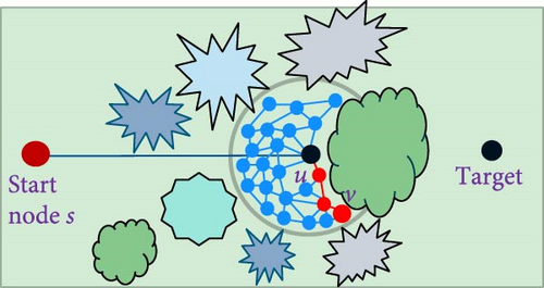
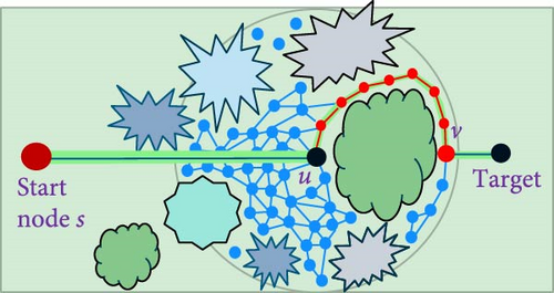
It is important to consider the obstacles size and accordingly determine the size of the enclosing circle. As the circle becomes larger, the likelihood of finding a detour path around the obstacle increases. On the other hand, enlarging the circle may affect the runtime. If the size of the obstacles on the map is unknown, the algorithm can be run multiple times with a predetermined circle size. If the algorithm fails to find a path or the success rate is very low, incrementally increase the circle radius and continue with that process until a satisfactory solution or a viable path is identified.

Figure 4 illustrates how circle size impacts the algorithm’s ability to find a path. Figure 4a shows a small circle relative to the obstacle. Here, the algorithm tries to find a detour but encounters a dead end, resulting in no path being identified. Figure 4b depicts a larger circle that encompasses the entire blocking obstacle, allowing the algorithm to successfully find a detour around it and identify a viable path.

The quality of the solution for PRM and its variants lies in the number of nodes placed on the map. While increasing the number of nodes improves the accuracy of the solution, it also increases the algorithm’s runtime and memory consumption. Figure 5 illustrates the advantages of TR-PRM, demonstrating its ability to reduce both the number of nodes and runtime without compromising the quality of the final route. This makes TR-PRM particularly valuable in applications where computational resources are limited or where a quick response is essential.

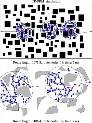
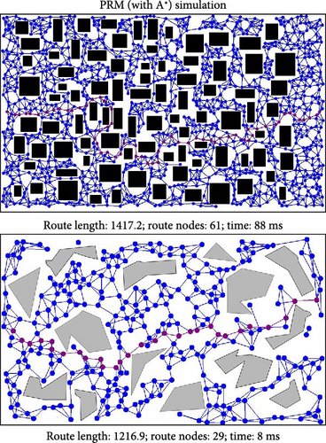
In the TR-PRM algorithm, nodes are added as needed for maneuvering when an obstacle is encountered. Thus, in more densely obstructed maps, the algorithm will allocate more nodes accordingly. Additionally, the algorithm benefits from processing each circle separately, breaking the problem into a series of smaller, quicker calculations that are then combined. This approach is more efficient than processing the entire map area at once. Simulation 1 up ahead examines this process in detail.

5.1.1. Simulation Experiment 1 (Tests of Node-to-Obstacle Ratio on Simulated Map)

In this simulation, PRM and TR-PRM were tested on a simulated map resembling the maps shown in Figure 4. The aim was to compare TR-PRM with PRM in terms of running time, number of nodes placed on the map, and length of the final route. To facilitate this comparison, we generated a 2000 × 500 px map and populated it with obstacles at densities ranging from 10% to 50% in steps of 10%. We then placed multiple nodes, each with a diameter of 10 px, so that they collectively occupied 20% of the map’s area. In the PRM algorithm, the number of nodes is fixed, whereas in TR-PRM, the number of nodes varies based on the map’s conditions. Table 1 highlights the efficiency of TR-PRM over PRM in terms of running time, number of nodes placed on the map, and the length of the final route.

Table 1. Comparisons of probabilistic roadmap (PRM) and target-oriented rapidly-exploring PRM (TR-PRM) based on various metrics, including running time, total number of nodes placed, and path length, calculated on randomly generated maps.

Obstacle density	Metric/algorithm	PRM	TR-PRM
10%	Run time (ms)	536	17
	Total nodes	2546	377.33
	Path length	2156.99	2074.82
20%	Run time (ms)	545	43
	Total nodes	2546	1003.41
	Path length	2250.49	2218.78
30%	Run time (ms)	570	78
	Total nodes	2546	1570.90
	Path length	2311.89	2279.15
40%	Run time (ms)	592	95
	Total nodes	2546	1767.96
	Path length	2331.25	2285.36
50%	Run time (ms)	613	108
	Total nodes	2546	1915.58
	Path length	2332.62	2292.31

The TR-PRM algorithm operates faster, uses fewer nodes, and produces a shorter path. This table clearly demonstrates the significant improvements we’ve achieved in these areas, ultimately leading to a more efficient and optimized solution.

5.1.2. Simulation Experiment 2 (Tests of Pathways in Real Urban Environments)

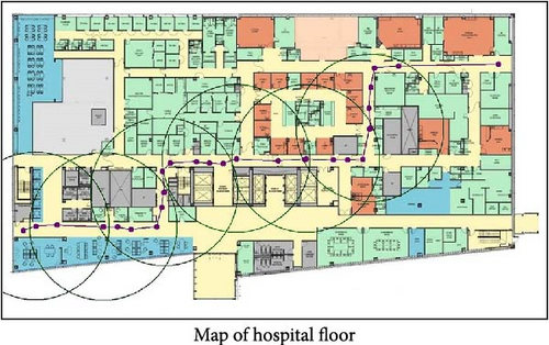
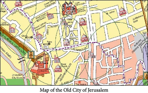
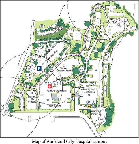
In these environments, the robot faces a cluttered navigation challenge, with significant obstructions from surrounding buildings forcing it to maneuver through curved and complex pathways, much like navigating through tunnel pipes, where it must establish a viable path to ensure smooth bidirectional flow through constrained spaces. Thanks to the TR-PRM approach, which focuses on the relevant working areas, the algorithm increases its chances of generating nodes at strategic locations, such as within complex passages. This local focus enables it to find routes quickly and efficiently in most cases. Figure 6 presents several visual examples of the TR-PRM algorithm applied to various sources, and Table 2 provides comparison results for those examples.

Table 2. Comparisons of several algorithms based on various metrics, including running time, final route length, and the corresponding number of nodes, for the examples in Figures 4 and 5.

Example	Metric/algorithm	PRM	Lazy	Gaussian	HPPRM	TR-PRM
Hospital floor (4.a)	Run time (ms)	39	36	54	11	12
	Path nodes	34.09	34.09	39.91	37.52	34.55
	Path length	1122.51	1122.51	1123.27	1380.00	1121.66
City map (4.b)	Run time (ms)	102	102	139	258	31
	Path nodes	61.73	61.73	67.64	73.57	67.81
	Path length	2284.65	2284.65	2294.26	2245.55	2281.92
Hospital campus (4.c)	Run time (ms)	39	36	65	77	15
	Path nodes	71.17	71.17	77.59	86.79	50.51
	Path length	1863.93	1863.93	1854.25	1856.25	1818.83
Circles (5.a)	Run time (ms)	11	11	11	5	2
	Path nodes	28.53	28.53	28.67	23.69	21.02
	Path length	570.05	570.05	564.34	596.84	552.70
Narrow (5.b)	Run time (ms)	29	29	34	13	5
	Path nodes	42.16	42.16	41.51	38.14	35.58
	Path length	497.61	497.61	471.10	517.13	457.35
Squares (5.c)	Run time (ms)	13	12	13	5	2
	Path nodes	39.09	39.09	38.81	30.45	24.48
	Path length	710.29	710.29	709.80	726.13	635.72

Figure 6a illustrates the floor plan of a real hospital in Michigan, United States. The corridors are highlighted in yellow, while all other areas are designated as obstacles. The solution obtained can assist nursing robots or transportation robots in navigating around patients and medical staff. Figure 6b illustrates the map of the Old City of Jerusalem. The streets are depicted with emphasis on their narrow and winding nature. The solution obtained can assist delivery robots or autonomous vehicles in efficiently navigating the tight and complex urban layout. Figure 6c illustrates the map of Auckland City Hospital campus in New Zealand. The map includes numerous parking lots and surrounding roads. The solution obtained can help an ambulance robot efficiently navigate between buildings on the hospital campus and move through the surrounding areas. The resulting paths are smooth and near optimal for all examples.

5.1.3. Simulation Experiment 3 (Tests of Narrow Passages on Simulated Maps)

Various articles address the challenge of navigating narrow passages between dense obstacles. In this analysis, we explore several examples from these studies, focusing on environments where obstacles have different shapes and sizes, which present significant navigation challenges due to their complex layouts. The TR-PRM approach proves particularly effective in these scenarios by targeting relevant working areas and generating nodes in strategic locations. This focused approach enables efficient pathfinding even in highly constrained spaces. Figure 7 provides visual examples of the TR-PRM algorithm from these sources, and Table 2 presents comparative results for the discussed scenarios.

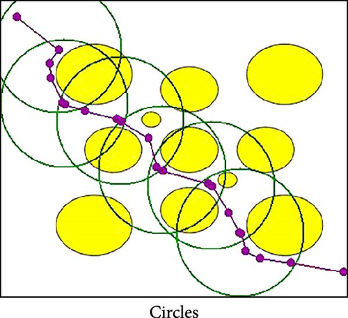
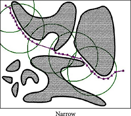
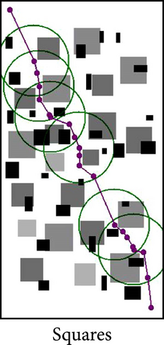
TR-PRM stays on course and excels in connecting paths through obstacles, whereas other algorithms often struggle with this task. They generally attempt to find routes around obstacles rather than through them, which leads to suboptimal solutions. For instance, in Figure 7a, the TR-PRM algorithm effectively navigates an environment with dense circular obstacles, demonstrating its robustness in handling complex configurations. In Figure 7b, which features a very narrow passage, finding a viable path is extremely challenging. Most algorithms, including PRM, Lazy, HPPRM, and Gaussian, required numerous repetitions before achieving a successful result. In contrast, TR-PRM demonstrated notably higher success in this scenario. Similarly, Figure 7c illustrates the algorithm’s capability to navigate through dense square obstacles, further showcasing its efficiency in resolving challenging layouts. Its approach of focusing on relevant working areas allows it to generate nodes at strategic locations, such as within narrow passages, thereby significantly improving pathfinding efficiency and achieving solutions where others fail. Table 2 presents the results for the examples depicted in Figures 6 and 7.

Results presented in Table 2 showcase the performance across a range of scenarios, highlighting that the TR-PRM algorithm consistently produces superior solutions compared to other tested alternatives in the average case. Not only does it achieve higher success rates in complex environments, but it also demonstrates a significantly shorter running time, making it a more efficient and reliable choice in navigating challenging spaces.

5.1.4. Simulation Experiment 4 (Testing of Algorithm Performance Under Varying Densities)

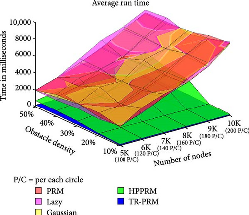
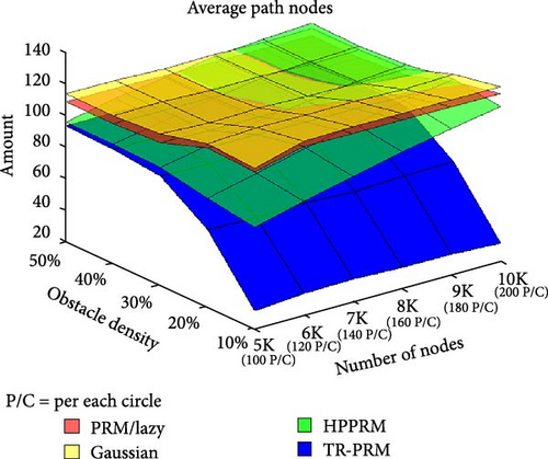
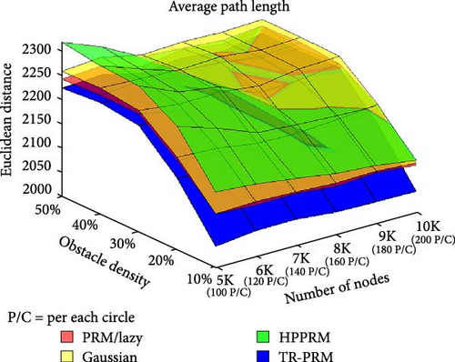
Figures 8–10 present statistical averages for PRM type algorithms, showcasing their performance on simulated maps of a long corridor with dimensions set to 2000 × 500 px. The maps include randomly placed average-sized obstacles. Statistical averages for runtime, number of nodes in the final path, and final path length are provided to offer a comprehensive overview of the algorithms’ performance in different test cases. These test cases were distinguished by diverse obstacle densities and a varying number of nodes allocated on the map, encompassing a substantial range: specifically, 5000, 6000, 7000, 8000, 9000, and 10,000 nodes. The obstacle density factor represents the proportion of the map area covered by obstacles, ranging from 10% to 50% in steps of 10%, while the number of nodes factor helps determine the accuracy of the solution. In the TR-PRM algorithm, the number of nodes within each circle corresponds to the density ratio of the nodes found in the entire map compared to competing algorithms. Put simply, it represents the average number of nodes that would appear within a randomly drawn circle on the map after running the PRM algorithm. This quantity of nodes in TR-PRM is denoted on the charts as P/C, indicating “per each circle.”

The selection of the map size, coupled with the ratio of obstacles and the number of nodes placed within it, poses a highly intricate calculation problem, demanding substantial time and memory resources. Through this comparison, we continue to fortify the assertion of the reliability, stability, and efficiency of the TR-PRM algorithm.

For each test case, we generated multiple distinct random maps and executed 300 runs for each algorithm, summing up to a collective total of 9000 runs per algorithm. Each plotted point on the graph represents the average outcome derived from these runs. Throughout the obstacle placement process, we took care to prevent any overlaps between obstacles and maintained sufficient distance between them to accommodate nodes. This method ensured that each random map produced was non-maze-like, allowing feasible solution paths to be found. For all simulations, we placed the source at left–middle position and defined 10 possible target points on the far-right side of the map.

In Figure 8, TR-PRM demonstrates exceptional runtime performance, highlighting a significant disparity compared to other PRM versions. This disparity becomes particularly apparent with larger numbers of nodes and obstacles, showcasing TR-PRM’s efficiency owing to its nonexploratory nature, enabling numerous algorithm executions. Additionally, TR-PRM generates fewer nodes and edges than other algorithms, contributing to its advantages in memory usage and computational requirements.

Moreover, if we extend the problem beyond the given scope, PRM and its variants will encounter significant issues. Either the running time escalates dramatically, or the application crashes due to running out of memory.

Another noteworthy observation from the graph is the variability in runtime efficiency exhibited by Lazy when contrasted with PRM and Gaussian. As the problem complexity increases, the comparative advantage of this algorithm diminishes. HPPRM achieves a significant improvement in runtime compared to standard approaches, as it allocates fewer nodes depending on the density of obstacles in the area.

Figure 9 depicts the count of nodes in the final path, reflecting the preference for routes with fewer intersections and turns, especially beneficial for robots requiring complex rotation operations. As the density of obstacles increases on the map, the ratios between different algorithms tend to converge, indicating similar performance under high obstacle density conditions. However, even amidst high obstacle density scenarios, TR-PRM manages to retain a discernible advantage, emphasizing its efficiency in generating paths with reduced nodes and enhanced navigational simplicity.

In Figure 10, we observe that the average path length ratio remains constant, with the path length in the TR-PRM algorithm being consistently shorter for all cases. This unwavering advantage suggests TR-PRM’s efficiency in consistently producing shorter paths regardless of the scenario’s complexities or variations in obstacle densities.

In summary, the TR-PRM algorithm excels with the best runtime and the best path length among the considered algorithms. Gaussian PRM aims to intelligently spread its nodes across key areas, yet the results indicate the least favorable outcome in this aspect. HPPRM increases the number of nodes on the map, due to the density of obstacles, the closer it gets to the solution obtained in PRM. Seemingly, in scenarios with randomly placed obstacles, the most effective approach involves random node placement. This aligns with the priorities of practical operational systems utilizing probabilistic algorithms, which often emphasize speed, efficiency, and memory usage. Given the need for multiple executions in such systems, TR-PRM stands out for its superior performance, offering the best runtime and path length, making it a preferred choice.

6. Summary and Conclusions

In this paper, we presented a practical modification for PRM called R-PRM, which enhances the traditional construction phase of the graph by incrementally building it from the starting point and selectively expanding only from reachable neighbors. This practical approach enhances the path search process and significantly eliminates excessive calculations. We also introduced a novel algorithm, Algorithm 3, which intelligently employs ray casting to explore multiple paths and identify the least obstructed direction; upon encountering an obstacle, it utilizes R-PRM as a sub-algorithm in the surrounding area to maneuver around it. TR-PRM algorithm demonstrates significant advantages over traditional PRM methods, offering efficient navigation in complex environments. Its advantage is that it avoids spanning the entire map, leading to noticeably quicker computations when compared to the tested alternative methods. Working with the algorithm requires attention to key parameters to ensure optimal performance. Specifically, the size of the obstacle-enclosing circles and the number of rays cast influence runtime and solution quality. These parameters should be carefully calibrated along with other PRM settings to maintain a balance between computational efficiency and path optimization. Dynamic scenarios may require evaluating environmental stability to preserve roadmap reliability.

TR-PRM was experimentally analyzed with various sampling strategies in diverse environments, particularly large, complex maps with thousands of nodes and obstacles. The analysis demonstrated superior results in computational time, path length, and solution accuracy compared to other probabilistic motion planning algorithms.

Conflicts of Interest

The authors declare no conflicts of interest.

Funding

The authors do not have any exterior funding for preparing this paper. The publication costs were covered by Holon Institute of Technology (HIT).