Comparison of Machine Learning Methods and Ordinary Kriging for Gravimetric Mapping: Application to Yagoua Area (Northern Cameroon)
Abstract
This work focuses on the comparison of a number of machine learning methods (random forest, support vector machine (SVM), and artificial neural networks (ANN)) and ordinary kriging (OK). It is based on OK. Indeed, OK, which is a stochastic spatial interpolation method, predicts the value of a natural phenomenon at unsampled sites, and it is an unbiased linear combination with a minimal variance that yields observations on the model at neighbouring sites. So, knowing the various improvements made by machine learning–based methods, we used them. The analysis of the different methods provides a basis for comparison according to the defined indicators. A better gravimetric mapping requires the sampling of a certain number of points whose densities will make it possible to carry out geostatistical analyses and interpretations and thus be able to estimate the deposit. Thus, concerning the prediction of the parameters used in the detection of gravity anomalies, OK is better with R2 = 0.99. Regarding the prediction of gravity anomalies, OK is able to reproduce a good variability of the anomalies, but when the spatial variability interval of the ANNs is close, it is then better indicated than OK. However, an increase in the data size would allow us to see the best performance of machine learning–based methods in gravity mapping.
1. Introduction
During the last two decades, machine learning has been increasingly applied in the geosciences, notably in the fields of geochemistry [1, 2], geomatics and geological mapping [3, 4], structural geology [5, 6], and also geostatistics [7, 8]. In geophysics, its application started in fault detection and prevention [9, 10], then extended to geological and mining fields through geoelectrics [11, 12], magnetics [13], and seismics [14, 15]. In gravimetry, the contribution of machine learning has been mainly for data inversion. For example, Chen et al. [16] used deep neural networks on Bouguer anomalies for the determination of the spatial structure of salt and concluded that the machine learning–based method from gravity data complements the processing and interpretation of seismic data for subsurface exploration. Next, a 3D inversion tool for gravity data was developed by Zhang et al. [17] for density determination. Instead of learning the density information of each 2D grid point as is often used, this network learns the boundary position, vertical center, thickness, and density distribution and reconstructs the 3D model using these predicted parameters [17]. Finally, in a study at Eastern Goldfields in Australia, random forest (RF) was combined with teledetection for lithological mapping, and it was concluded that the method can be an effective additional tool available to geoscientists in a pristine gold-bearing environment when faced with limited data [18]. The Northern Cameroon region has been the subject of previous research in the geophysical framework [19–24]. This paper builds on the work of Nouck et al. [25], which focused on the geostatistical reinterpretation of gravity surveys in the Yagoua area. The contribution of this paper is to use machine learning–based methods to improve gravimetric mapping. The main idea is to leave the so-called classical methods, such as ordinary kriging (OK), to go towards RF, support vector machine (SVM), and artificial neural network (ANN). A comparison is then made according to certain defined indicators.
The rest of this article is organized as follows: Section 2 presents a review of gravity mapping. Section 3 shows the geological setting of the study area. Section 4 presents the conceptual and methodological framework of this work. Section 5 presents the results obtained and discusses them. Finally, Section 6 presents a conclusion and perspectives related to this work.
2. Survey of Gravimetric Mapping
Gravimetry is a geophysical method that measures variations in the Earth’s gravitational potential field [26]. It is a prospecting method that offers the determination of density anomalies in the subsurface. Depending on the objectives and the means available, there are several gravity surveys: land, sea, airborne, and satellite gravity surveys. In the context of this work, the focus is on terrestrial gravity surveys. Better gravity mapping requires the sampling of a certain number of points whose densities will allow geostatistical analyses and interpretations to be carried out and thus be able to estimate the deposit. There are few works that abound on topics related to gravimetric mapping. Figure 1 shows the steps required for good gravimetric mapping.
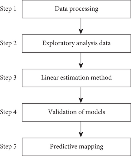
In this work, we focus on the third step: the use of linear estimation methods. Indeed, this is a set of methods used for the estimation of regionalized stationary variables [27]. We build on the work of Nouck et al. [25]. The method used in their work was based on variographic analysis and OK.
2.1. OK
However, the emergence of new technologies in data engineering and artificial intelligence is challenging the results obtained in many fields of activity. Even geostatistical methods are not to be spared. Several studies have shown the limitations of kriging [30]. Indeed, kriging uses simple criteria that do not allow confidence intervals to be characterized. Kriging-based methods apply smoothing to the variability of the data. This could lead to estimation errors. Machine learning is then an alternative for the improvement of geostatistical estimates, including their application to gravity mapping. Machine learning is an application of artificial intelligence that aims to have systems learn and improve from experience without being programmed [9]. The objective of this paper is to make a comparative study of the estimates made with OK and some machine learning methods (RF and ANN) for gravimetric mapping. Before doing so, it is therefore important to present the study area.
3. Geological Framework of the Study Area
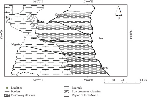
The study area used for this work is a vast sandy plain located between longitudes 15°148 ′ and 15°354 ′ E and latitudes 10°12 ′ and 10°395 ′ N (Figure 2). It covers the locality of Yagoua and its surroundings. Located about 211 km from Maroua, this area is bounded by the Logone River and therefore borders Chad. The whole area is easily accessible by land. It is mostly made up of sedimentary cover of tertiary and quaternary age. The sediments are mainly sandstone, clay, and shale and are overlain by sandy-alluvial and dune formations [25]. These sedimentary deposits are the result of a succession of regressions and transgressions caused by alternating periods of no rainfall and rainy periods.
4. Methodology
4.1. Proposal Design
Figure 3 shows the approach used in this work to compare the methods we are using in order to produce a better predictive map.
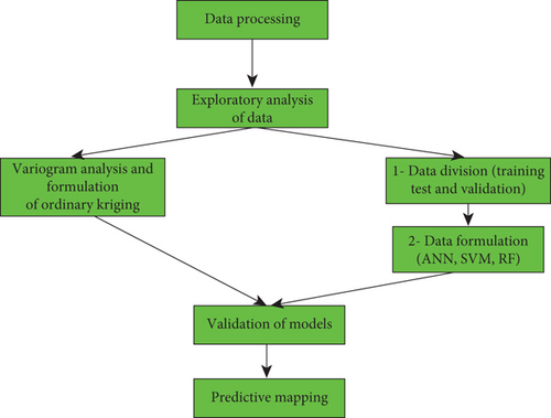
For this work, it is chosen, on the one hand, to use OK, as realized by Nouck et al. [25], and, on the other hand, three methods based on machine learning, namely, RF, ANN, and SVM. Subsequently, model validation methods are used to assess the most suitable method, and finally, the gravimetric map is generated using the best method.
4.2. Machine Learning Methods Used
4.2.1. RF

4.2.2. ANN
- •
the sum of all input variables
- •
the weighting factor feeding these nodes
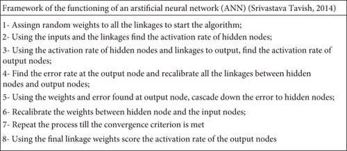
In addition, there may be a bias term that behaves similarly to the intersection in a typical linear regression. The following framework summarises the functioning of an ANN [38]:
4.2.3. SVM
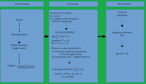
This is a computer algorithm that learns by example to assign labels to objects [39]. It represents a great technique for general (nonlinear) classification and outlier detection by using an intuitive model representation. SVM approaches are summarised as follows [40]: nonlinearity, class separation, overlapping, one-class classification, and multiclassification. Several problems today have their solutions improved thanks to SVM. The literature abounds with works that exploit the SVM method. In this work, we are interested in the use of SVM in the process of estimating reserves in the mining and petroleum domain. In estimating ore reserves from sparse and imprecise data, Dutta et al. [8] use several automatic learning methods, including the SVM method. This method allows for predicting the drilling parameters in a minimal way and obtaining a good estimate of the reserve. Wong et al. [41] use SVM methods for reservoir characterization in an intelligent way using the petrophysical properties of reservoirs. Figure 6 shows the structure of the SVM algorithm [41].
4.3. Model of Cross-Validation
Validation models are those used to evaluate the performance of this type of mathematical model. Generally, in machine learning, it is to separate the database into three groups. The first part is used for training, the second is for testing, and the third is for model validation. Then, an estimation error is calculated by cross-validation according to certain parameters [42, 43]. Three validation methods are used in the validation of geostatistical and machine learning prediction models: the coefficient of determination (R2), the mean absolute error (MAE), and the root mean square error (RMSE).
4.3.1. Coefficient of Determination
4.3.2. Mean Absolute
4.3.3. RMSE
5. Results
5.1. Exploratory Data Analysis
A basic statistical analysis is carried out on the data in order to visualize their overall trend. A total of 104 points will be used for this study, and the results of which are presented in Table 1. This analysis has made it possible to summarise and synthesize the information contained in the statistical series and to highlight its properties. As can be seen in Table 1, the different statistical parameters calculated illustrate the degree to which the sampled data tend to deviate with a standard deviation of 1295 and a variance of 1.676∗106. These anomalies have a mean of −4471 mgal and range from a minimum value of −6643 mgal to a maximum value of −1090 mgal.
| Min. | Max. | Mean | Std dev. | Total |
|---|---|---|---|---|
| −6643.00 | −1090.00 | −4471 | 1295 | 104 |
The histogram in Figure 7 divides the statistical series of anomalies into different classes. These different classes of anomalies are represented on the abscissa, and the values on the ordinate indicate the frequency of anomaly data belonging to this class. Thus, in the case of our dataset, we have 12 classes represented. The mode of this series is the class (−5000 mgal; −4600 mgal). This implies that the majority of our anomalies have variations within this range.
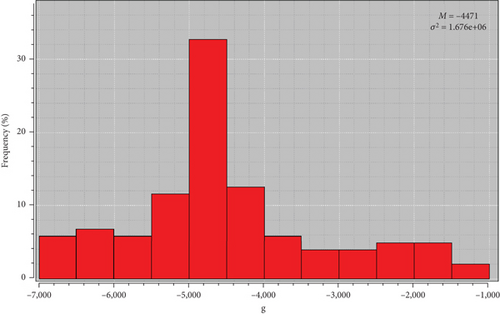
The distribution is positively skewed because the frequencies decrease much more to the right. So the anomalies do not follow a Gaussian distribution. In order to better examine the spatial continuity of the anomalies, it would be important to study the variogram and the variogram map.
5.2. Model Formulation
5.2.1. Variogram Analysis
This map (Figure 8) allows one to examine the spatial correlation of the anomalies in the four directions of space. A cell in this variogram map represents a family of point pairs with equal directions and distances between points. The value of the cell represents the value of the variogram for that family of pairs, and these values vary between 1512.50 and 1307943.61. This map shows the presence of a strong major anisotropy along the N20 direction, and we also note a minor N290 direction. These directions will be considered for the theoretical fitting of the experimental variogram.

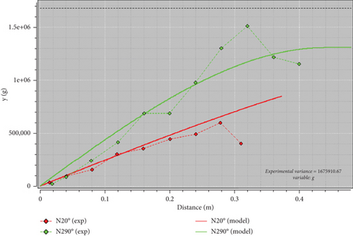
Figure 9 shows the representation of the experimental and theoretical variograms. Two experimental variograms have been plotted along the N20 direction (red dotted line) and the N290 direction (green dotted line). The red line represents the fit of the two experimental variograms. It results from the superposition of the two variograms with different ranges; it is a jiggly structure.
5.2.2. Hyperparameter Tuning
Hyperparameter optimisation is critical for maximising the predictive performance of machine learning models. This study explored the optimal configuration of key hyperparameters for SVMs, ANNs, and RFs using grid search cross-validation. Table 2 summarises the hyperparameter search ranges, their descriptions, and the best values identified, along with the corresponding model performance metrics.
| Model | Parameter | Search range | Description | Best value |
|---|---|---|---|---|
| SVM | Kernel | [“linear”, “rbf”] | Specifies the kernel type for transforming data. | “rbf” |
| C | [0.1, 1, 10] | Regularisation parameter controlling the trade-off between margin maximisation and classification error. | 10 | |
| Gamma | [0.01, 0.1, 1] | Kernel coefficient defining the influence of individual data points in nonlinear models. | 0.1 | |
| ANN | Hidden layer sizes | [(50, 50), (100,), (100, 100)] | Number of neurons in each hidden layer. | (100, 100) |
| Activation | [“relu”, “tanh”] | Nonlinear transformation function applied within layers. | “relu” | |
| Alpha | [0.0001, 0.001, 0.01] | L2 regularisation parameter to prevent overfitting. | 0.0001 | |
| Random forest | Number of trees (n_estimators) | [100, 200, 500] | Number of decision trees in the ensemble. | 500 |
| Maximum depth | [None, 10, 20] | Maximum depth of each decision tree to control overfitting. | 20 | |
5.3. Model Validation
In order to properly predict anomalies by using four models, it is important to validate the different models. The validation of each approach is done according to the method used.
5.3.1. Validation of OK
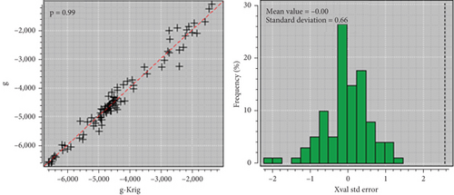
Figure 10 shows the correlogram between the true and estimated values on the left and the error histogram of the estimate on the right. The red bisector of the correlogram separates the true values from the estimated values. It can be seen that the correlation coefficient is 0.99 and the correlation cloud is tighter. This is one of the criteria to be taken into account to authenticate a good estimate because the closer the correlation is to 1 with a tighter cloud, the better the quality of the model. We can also visualize the histogram of the errors of the OK, where the average values of these errors have a major frequency of around 0 and the standard error is 0.66, showing that the estimation made is good.
5.3.2. RF Validation
The three graphs in Figure 11 show the relevance of the linear character that exists between the true values and the estimated values. These will allow you to validate the model by their behaviour. Our dataset allowed us to train and test the RF algorithm by the k-fold method in order to validate it. This graphical representation shows a good correlation with a value of R2 of 0.91 between the anomalies predicted by this model and the real values.
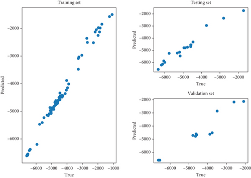
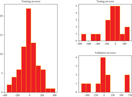
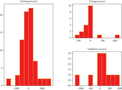
Figure 12 represents the histograms of the errors of the data that have been trained, tested, and validated. On these different histograms of the trained, tested, and validated data, the modes of the errors are very close to 0, reflecting that the mean of the errors is also close to 0, and therefore, we have a good fit for the model.
5.3.3. Validation ANN
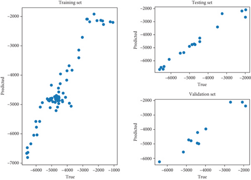
We can notice here a correlation R2 of 0.96, translating to a good quality of the prediction made by the ANN algorithm approach. Some of the predicted data are linearly close to the real anomalies, showing the robustness of this model. Figure 13 shows the linear link between the predicted and the measured data using ANN validation.
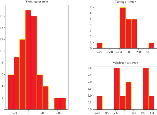
When looking at the error histograms shown in Figure 14, it can be seen that there is a fluctuation in the mean error in each case of the histogram, reflecting an instability in the mean error but not far from 0.
5.3.4. SVM Validation
The correlation is 0.88, illustrating a fairly strong correlation between the predicted anomalies and the actual anomalies, so we can speak of a fairly good fit for the SVM model.
The histograms in Figure 15 show a very low average error for each of the data, which is very close to 0, illustrating the quality of the prediction of these anomalies, as the lower the error, the better the model.
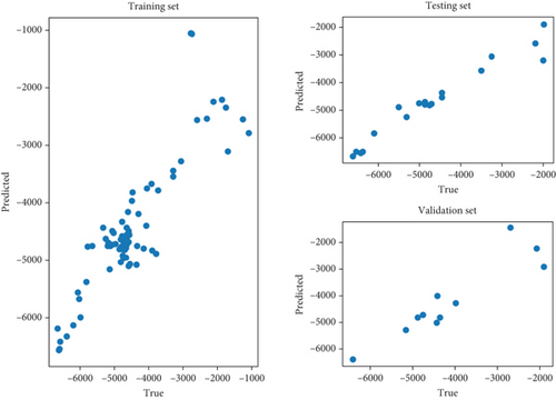
Figure 16 shows the validation model using SVM. In order to compare the four different approaches used, several parameters were determined, including R2, RMSE, MAE, and σe. These will allow us to identify the best performing model among the four. Table 3 gives the different values of the parameters calculated for each method used, including the variogram, RF, ANN, and SVM. We note R2 of 0.99, which translates to the good quality of the OK because it is stronger compared to the other models; RMSE of 221.86; and σe of 0.66, which are lower, showing the best performance. In view of these different parameters, the OK method is the best for the prediction of gravity anomalies.
| R2 | RMSE | MAE | σe | |
|---|---|---|---|---|
| Variogram model | 0.99 | 221.86 | 0.66 | |
| RF | 0.91 | 397.51 | 271.6 | 396.08 |
| ANN | 0.96 | 369.3023 | 291.5606 | 359.6318 |
| SVM | 0.88 | 564.8996 | 399.8502 | 559.1238 |
5.4. Predictive Maps
Once the prediction was made, each model was plotted on a map to better visualize the gravity anomalies. Figure 17 represents the prediction map obtained by the RF algorithm, and the estimated anomalies vary, respectively, between −6721.17 and −1121.87 mgal from blue to red. The strong anomalies are located to the east, and the weak ones are located to the west in relation to the north of this study area.
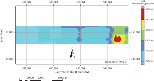
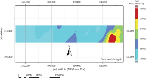
The gravity anomalies estimated by OK fluctuate between −6721.17 and −1121.87 mgal in contrast to those predicted by RF. A quick look at the results obtained by the RF allows one to observe that the tools have guessed wrong about the proper spatial variability of the body given the contrast of the measured gravimetric data. In the upper map, the data seems to be lumped per block or per area, which means that with this method applied to gravimetric data, we can at least guess the limitation of the bodies in the investigated field. The OK has the strong asset that it tends to minimize the variance of the predicting error, which means that all predictions are likely to be close to their expectation if we were working with a continuously complete series of gravimetric measurements. That way, one would better appreciate the spatial variability of the gravimetric information and then would be able to interpret that properly, depending on the geology of the investigated area.
The prediction by the ANN algorithm used as a model for anomaly mapping is shown in Figure 18 as a map. The predicted values vary from −7112.54 to −1666.83 mgal, totally different from the minimum and maximum of OK and RF. Indeed, because the OK tends to bring all the predictions to a mean, it is normal that the prediction from it will be tight in range compared to a brute method, such as ANN, which in this case, unlike the latter, runs a forecasting that uses a complex system of correlation between the measurements to provide the more realistic possible value for one prediction. Solely, the lack of information may be cruel for the ANN, which usually demands a lot of data to train the neural system. Despite the scarce amount of information, the ANN can still perform good prediction faster than the OK, and one may even observe that the spatial distribution of the gravimetric data seems to be quite close for both methods. It is also observed that the anomalies between −4389.68 and −3845.11 mgal are in the center, but the strong ones are on the extreme right, and the weak ones are on the extreme left.
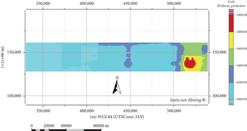
The map obtained by SVM is shown in Figure 19 with the estimated values varying between −7058.71 and −1028.55 mgal. It can be seen that these predicted values are closer to the ANN model than to the OK and RF models.

Figure 20 shows the prediction map obtained by OK. Finally, it is obvious that because of the spatial correlation embedded in the OK, the prediction can offer an appropriate observational product with a good spatial resolution to afford good interpretation from geophysicists as well as from geologists. However, if looking for quick observational products, or when the database starts growing fast, the use of the OK becomes less appropriate to fulfill the demand.
6. Conclusion and Future Work
The objective of this work was to provide information on machine learning methods for gravity mapping using RF, SVM, and ANN methods in the Yagoua region (Northern Cameroon). The mathematical foundations of the different methods were examined and compared in order to provide support for a reliable variographic analysis for interpolation issues. The choice of these methods allowed us to verify that the existing data was the same when modelling. Finally, it is clear that due to the integrated spatial correlation, OK seems to be good at prediction. Despite the limited information, ANNs can make good predictions faster than OK, and it can even be observed that the spatial distribution of the gravity data seems to be quite close for both methods. Prediction can provide a suitable observational product with good spatial resolution to allow good interpretation by geophysicists and geologists on future exploration projects. In addition, geostatistics gives an overview of the estimation from different interpolation techniques for locating, estimating, and simulating reserves.
Conflicts of Interest
The authors declare conflicts of interest.
Funding
This work has not received any funding.
Open Research
Data Availability Statement
The data used to write this article is confidential. It may be made available if necessary.


