This study investigates the forecasting of the Deutscher Aktienindex (DAX) market index by addressing the nonlinear and nonstationary nature of financial time series data using the CEEMDAN decomposition method. The CEEMDAN technique is used to decompose the time series into intrinsic mode functions (IMFs) and residuals, which are classified into low-frequency (LF), medium-frequency (MF), and high-frequency (HF) components. Long short-term memory (LSTM) networks are applied to the MF and HF components, while the backpropagation neural network (BPNN) is utilized for the LF components, resulting in a robust hybrid model termed CEEMDAN-LSTM-BPNN. To evaluate the performance of the proposed model, we compare it against several benchmark models, including ARIMA, RNN, LSTM, GRU, BIGRU, BILSTM, BPNN, CEEMDAN-LSTM, CEEMDAN-GRU, CEEMDAN-BPNN, and CEEMDAN-GRU-BPNN, across different training–testing splits (70% training/30% testing, 80% training/20% testing, and 90% training/10% testing). The model’s predictive accuracy is measured using six metrics: root mean squared error (RMSE), mean absolute error (MAE), mean absolute percentage error (MAPE), symmetric mean absolute percentage error (SMAPE), root mean squared logarithmic error (RMSLE), and R-squared. To further assess model performance, we conduct the Diebold–Mariano (DM) test to compare forecast accuracy between the proposed and benchmark models and the model confidence set (MCS) test to evaluate the statistical significance of the improvement. The results demonstrate that the CEEMDAN-LSTM-BPNN model significantly outperforms other methods in terms of accuracy, with the DM and MCS tests confirming the superiority of the proposed model across multiple evaluation metrics. The findings highlight the importance of combining advanced decomposition methods and deep learning models for financial forecasting. This research contributes to the development of more accurate forecasting techniques, offering valuable implications for financial decision-making and risk management.

1. Introduction

A time series is a collection of data points that are gathered or recorded at different times in time [1–3]. Time series analysis is essential to the finance industry because it helps analysts, investors, and policymakers comprehend and predict financial market movements. Financial markets are dynamic and so naturally unpredictable, with prices impacted by a range of factors such as macroeconomic trends, market mood, political developments, and economic indicators. For trading, risk management, and portfolio optimization to be done with knowledge, accurate forecasting of financial time series data is necessary [4, 5].

Forecasting stock prices [6–10], market indices [11, 12], exchange rates [13, 14], and other financial metrics are among the financial contexts where time series data is especially helpful. It makes it possible to systematically examine past data in order to spot trends and patterns that can direct future investment plans. Among the many uses of time series analysis, predicting stock market indices is crucial since they act as standards for market performance and offer important information about the state of the economy as a whole.

In finance, econometric models have been widely employed to evaluate time series data. For modeling and forecasting time series, traditional econometric techniques like generalized autoregressive conditional heteroskedasticity (GARCH) [15–17] and autoregressive integrated moving average (ARIMA) [18, 19] offer fundamental approaches. Nevertheless, these models frequently have trouble handling data that is nonstationary and nonlinear, which are features of financial time series. Because of this, they might not be able to accurately foresee the intricate relationships present in market dynamics.

The advent of machine learning (ML) has revolutionized financial forecasting by offering powerful tools to model nonlinear relationships and complex interactions within time series data [20–25]. Among the ML techniques, deep learning (DL) models, such as long short-term memory (LSTM) networks and gated recurrent units (GRUs) with their variants, have gained significant traction due to their ability to learn from large datasets and capture intricate temporal dependencies [26–29]. These models can automatically adjust their parameters during training, allowing them to adapt to varying patterns in financial data, thus enhancing their predictive accuracy.

Because econometric models have solid theoretical underpinnings and can accurately represent linear connections and volatility in financial data, they have traditionally been preferred for time series forecasting. They are perfect for conventional financial analysis since they are interpretable and perform well with stationary time series. However, by successfully identifying nonlinear patterns and dependencies in sequential data—especially in intricate, nonstationary time series—ML models have completely transformed forecasting. Unlike econometric models, which are based on strict assumptions, these models are able to handle enormous amounts of data and learn complex properties. However, both approaches have limitations: econometric models struggle with nonlinearity and nonstationarity, while ML models can suffer from overfitting and lack interpretability. Hybrid modeling has garnered significant research interest because it combines the strengths of different methods, allowing for more accurate, flexible, and interpretable financial forecasting by addressing the individual weaknesses of each approach. This combination leads to more robust models capable of handling the complex dynamics of financial markets.

Hybrid modeling in time series forecasting involves combining different methodologies to harness the strengths of each for improved prediction accuracy, particularly in complex domains like finance. In recent years, hybrid models that integrate econometric models with ML techniques have gained attention. These approaches capitalize on the explanatory power of traditional statistical models (like ARIMA, GARCH, or VAR) while addressing their limitations, such as linearity assumptions, by incorporating the flexibility and adaptability of ML [30, 31]. These hybrid models offer the best of both worlds, enabling more robust and interpretable predictions in the finance sector.

Hybrid models of ML and DL, which integrate many architectures, have also been investigated to improve time series forecasting. These methods use the strengths of different ML models in identifying nonlinear patterns and sequential relationships in financial data [32–34]. In time series forecasting, decomposition–ensemble hybrid models have become more and more common, particularly in the banking industry where data frequently display chaotic, nonlinear patterns with abrupt jumps and asymmetries. In order to overcome the difficulty, these models first decompose the intricate time series into easier-to-manage parts. For this task, methods such as empirical mode decomposition (EMD) [35–40], its improved version ensemble empirical mode decomposition (EEMD) [41–43], complete ensemble empirical mode decomposition with adaptive noise (CEEMDAN) [44–46], and variational mode decomposition (VMD) [47–50] are frequently employed. The original series is broken down into intrinsic mode functions (IMFs) or other modes that capture patterns at low, mid, and high frequencies by decomposition. By separating these elements, ML models such as LSTM, GRU, and BPNN (backpropagation neural network) may more easily estimate trends unique to each frequency or IMF, which are then combined to create a final forecast. This multistep approach of dissecting and reassembling the forecast enhances performance by concentrating on various time series features, guaranteeing greater flexibility in response to abrupt changes and anomalies in the market [44–46, 51].

Among decomposition techniques, CEEMDAN stands out for its ability to mitigate the issue of mode mixing, where similar frequencies overlap in different IMFs, leading to poor model interpretability and degraded forecasting performance. CEEMDAN introduces adaptive noise to resolve mode mixing, allowing for clearer separation of components, which results in more accurate predictions. In comparison to simpler methods like EMD or even wavelet transforms, CEEMDAN has proven superior in terms of handling the inherent nonlinearity and chaotic nature of financial time series. This decomposition method has consistently shown improved results in forecasting models, particularly when paired with neural networks, as it reduces noise and better captures the underlying signals in market data. However, while decomposition–ensemble methods have demonstrated promise, the application of these advanced techniques, particularly in forecasting market indices, remains relatively underexplored. There is substantial potential to enhance forecasting accuracy by refining hybrid models using decomposition techniques in future research. Therefore, in this study, we focus on the Deutscher Aktienindex (DAX) market index, which is a critical indicator of the German stock market’s performance. The DAX index is characterized by its nonlinear and nonstationary behavior, posing challenges for accurate forecasting. To address these challenges, we employ the CEEMDAN technique, which effectively decomposes the time series into IMFs and a residual component. This decomposition categorizes the components into low frequency (LF), medium frequency (MF), and high frequency (HF), allowing for a more nuanced analysis of the underlying patterns in the data.

The proposed CEEMDAN-LSTM-BPNN model utilizes LSTM networks for the MF and HF components, while employing a BPNN for the LF components. This innovative combination allows the model to leverage the strengths of each method, resulting in a robust and accurate forecasting framework. By integrating the CEEMDAN decomposition with advanced neural network architectures, we aim to improve the predictive performance of financial time series forecasting.

This research makes several key contributions to the field of financial time series forecasting. First, it introduces a novel hybrid model CEEMDAN-LSTM-BPNN designed to handle the inherent nonlinear, nonstationary, and chaotic nature of financial data by decomposing it into more predictable components. Second, the model integrates CEEMDAN for decomposition, LSTM for MF and HF components, and BPNN for LF components, creating a robust architecture that outperforms benchmark methods. Third, the study conducts a rigorous evaluation across three forecast horizons: 70% training/30% testing, 80% training/20% testing, and 90% training/10% testing splits, allowing for a comprehensive assessment of the model’s adaptability over different time frames. Fourth, it employs six performance metrics—root mean squared error (RMSE), mean absolute error (MAE), mean absolute percentage error (MAPE), symmetric mean absolute percentage error (SMAPE), root mean squared logarithmic error (RMSLE), and R-squared—ensuring a detailed evaluation of both accuracy and error distribution.

To further validate the robustness of the proposed model, Diebold–Mariano (DM) and model confidence set (MCS) tests were employed. The DM test compares the predictive accuracy of two competing models, testing whether the forecast errors of the models differ significantly. The null hypothesis of the DM test states that the two models have equal predictive accuracy, while the alternative hypothesis suggests that one model outperforms the other. On the other hand, the MCS test provides a set of models that are considered statistically indistinguishable in terms of forecast accuracy, allowing for a comparison of multiple models simultaneously. Together, these tests provide a rigorous framework to assess whether the proposed CEEMDAN-LSTM-BPNN model significantly improves forecasting accuracy over benchmark methods.

The manuscript is organized as follows: Section 2 outlines data and the methodologies employed in the study. Section 3 discusses the results of the proposed model and compares its performance with benchmark models. Section 4 concludes the research by summarizing the findings, and Section 5 highlights future study directions.

2. Data and Methods

2.1. Data

For this research, we utilized the daily closing prices of the DAX index, spanning from August 1, 2004, to August 31, 2024. The DAX index is a stock market index consisting of the 40 major companies listed on the Frankfurt Stock Exchange. The daily closing prices of this index were selected because they serve as a reliable indicator of the market’s performance at the end of each trading day, which is crucial for financial forecasting and analysis.

Closing prices are widely used in financial research because they reflect the final consensus value of an asset, providing an accurate snapshot of its worth. These prices are often considered more stable and less influenced by intraday market fluctuations compared to intraday data. Therefore, they are a preferred choice for time series analysis in market research and performance evaluation.

The data was obtained from Yahoo Finance 1, a widely used platform for accessing historical stock market data.

2.2. CEEMDAN

CEEMDAN is an enhanced time series decomposition technique that refines EMD by mitigating mode mixing through adaptively injected noise. Unlike EMD, EEMD, AkimaEMD, and Statistical-EMD, CEEMDAN ensures a more stable and accurate decomposition by systematically controlling noise dispersion, preserving signal integrity, and improving component separation [44–46, 52].

The CEEMDAN procedure follows these steps.

First, additive white Gaussian noise η_j(t) is incorporated into the original signal s(t) to create ensemble realizations:

(1)

where M is the number of realizations.

Next, EMD is applied to each realization s_j(t) to obtain the first IMF:

(2)

The first IMF is computed as the mean across all ensemble realizations:

(3)

The first residual component is then determined by subtracting ψ₁(t) from s(t):

(4)

For subsequent IMFs, adaptive noise is added to the residual from the previous step:

(5)

Applying EMD to

extracts the k-th IMF:

(6)

Averaging across all realizations gives

(7)

The residual is updated as

(8)

The process continues until all significant IMFs are extracted. The original signal can be reconstructed as

(9)

where N is the total number of IMFs and r_N(t) is the final residual.

This refined decomposition method enhances feature extraction and improves predictive accuracy, making CEEMDAN a more effective approach for financial time series analysis.

2.3. Recurrent Neural Networks (RNNs)

RNNs [53] are designed to handle sequential data by maintaining a hidden state that evolves with each time step. However, traditional RNNs struggle with long-term dependencies due to the vanishing and exploding gradient problems. At each time step t, the hidden state h_t is updated as

(10)

where h_t is the hidden state at time t, h_t−1 is the previous hidden state, x_t is the input at the current time step, W_h is the weight matrix, and b_h is the bias term. The activation function σ (typically a sigmoid or tanh) determines the output of the hidden layer.

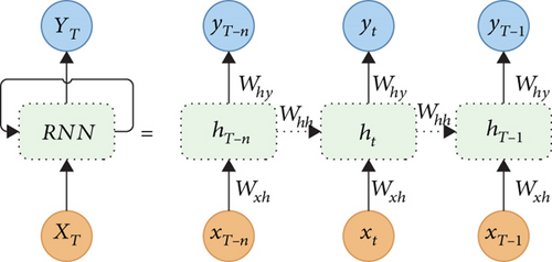
Despite their ability to process sequential data, RNNs fail to retain long-term information over extended sequences, as the gradients during backpropagation either vanish or explode. This limitation is addressed in LSTM and GRU and their variant networks, which employ specialized gates to better capture long-range dependencies and regulate the flow of information. Figure 1 shows the RNN layout.

Details are in the caption following the image — **Figure 1**
Open in figure viewer PowerPoint

Architecture of RNN.

2.4. LSTM

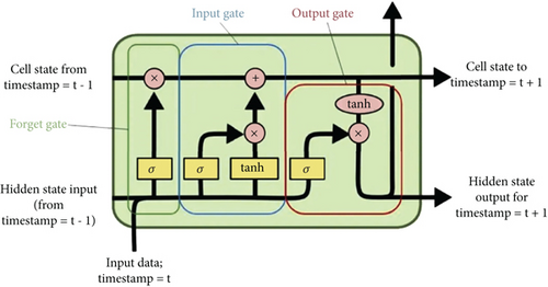
LSTM networks are designed to overcome the limitations of traditional RNNs by introducing a set of gates that govern the storage, modification, and removal of information. At each time step, the LSTM processes the current input x_t, the previous hidden state h_t−1, and the previous cell state C_t−1 to compute the updated values of the cell state and hidden state.

The forget gate, denoted by f_t, controls how much of the previous cell state C_t−1 should be remembered. It is computed as

(11)

where W_f is the weight matrix, b_f is the bias, and σ is the sigmoid activation function that outputs values between 0 and 1.

The input gate i_t determines the amount of new information to be added to the cell state, and the candidate cell state

provides a potential update to the cell state. These are computed as

(12)

(13)

where tanh is the hyperbolic tangent function that outputs values between −1 and 1.

The cell state C_t is then updated by combining the previous cell state C_t−1, modulated by the forget gate, and the new candidate cell state, scaled by the input gate:

(14)

where ⊙ represents element-wise multiplication.

The output gate o_t determines the new hidden state h_t, which is both the output of the current time step and input to the next:

(15)

(16)

The forget gate f_t controls what information is discarded from the cell state, the input gate i_t controls what new information is added, and the output gate o_t regulates the hidden state h_t. This gating mechanism enables the LSTM to effectively capture long-term dependencies in sequential data by preventing the vanishing gradient problem that affects traditional RNNs [26–29]. Figure 2 shows the LSTM layout.

2.5. GRU

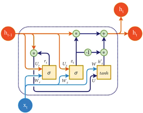
The GRU is a more efficient variant of the RNN designed to overcome long-term dependency issues with fewer gates and reduced computational complexity compared to LSTM networks. GRU merges the functionalities of the forget and input gates in LSTM into a single update gate. This simplification allows it to achieve similar performance in many tasks, making it highly effective for sequence modeling [26–29].

At each time step t, the GRU uses the update gate z_t to regulate how much of the past hidden state h_t−1 should be carried over to the current time step. The update gate is calculated as

(17)

where σ is the sigmoid activation function, W_z is the weight matrix for the update gate, b_z is the bias term, h_t−1 is the previous hidden state, and x_t is the current input at time t.

The reset gate r_t determines how much of the previous hidden state should be ignored when computing the candidate hidden state. It is given by

(18)

where W_r is the weight matrix for the reset gate and b_r is the bias term for the reset gate.

The candidate hidden state

is calculated using the reset gate r_t to modulate the influence of the previous hidden state. The candidate hidden state is computed as

(19)

where tanh is the hyperbolic tangent activation function, W_h is the weight matrix for the candidate hidden state, b_h is the bias term for the candidate hidden state, and ⊙ represents element-wise multiplication.

The final hidden state h_t is computed as a weighted sum of the previous hidden state h_t−1 and the candidate hidden state

, controlled by the update gate z_t. It is given by

(20)

Figure 3 shows an illustration of a GRU cell.

2.6. Bidirectional GRU (BIGRU)

The BIGRU extends the standard GRU by processing data in both forward and backward directions [50, 54]. This dual processing allows the model to capture context from both the past and future, improving the model’s ability to understand the temporal dependencies in sequential data. In the forward direction, the BIGRU computes the hidden state as

(21)

where

is the forward hidden state and W_z and b_z are the weight matrix and bias term for the forward direction.

Similarly, in the backward direction, the BIGRU computes the hidden state as

(22)

where

is the backward hidden state and W_z and b_z are the weight matrix and bias term for the backward direction.

The final combined hidden state h_t is formed by concatenating the forward and backward hidden states as follows:

(23)

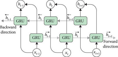
Figure 4 shows an illustration of a BIGRU cell.

2.7. Bidirectional LSTM (BILSTM)

The BILSTM is a variant of the LSTM that processes the data in both forward and backward directions [55, 56]. This architecture helps capture dependencies in both directions, improving the model’s performance for tasks such as sequence labeling and speech recognition. In the forward direction, the BILSTM computes the hidden state as

(24)

where

is the forward hidden state and LSTM represents the LSTM cell.

In the backward direction, the BILSTM computes the hidden state as

(25)

where

is the backward hidden state.

The final hidden state h_t is formed by concatenating the forward and backward hidden states as follows:

(26)

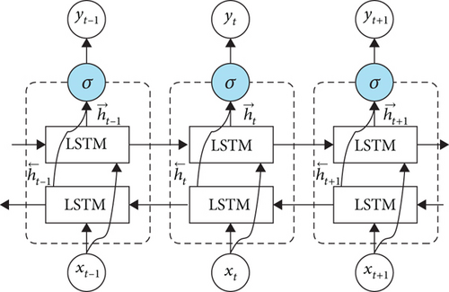
Figure 5 shows an illustration of a BILSTM cell.

2.8. Backpropagation in Neural Networks

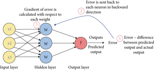
Backpropagation is a supervised learning algorithm commonly employed in training artificial neural networks. It optimizes the network by iteratively adjusting its weights to minimize the error between the actual output and the predicted output. This is achieved by propagating the error backward through the layers and updating the weights using gradient descent [39, 40, 57].

The training process of backpropagation consists of the following stages.

In the forward pass, input data is passed through the network layer by layer, using the activation function at each layer to compute the output of the neurons. The network’s predicted output y^p is generated by the final layer.

To quantify the discrepancy between the predicted output y^p and the actual output y^a, a loss function L is defined. For regression tasks, the mean squared error (MSE) is often used:

(27)

where n is the number of observations.

The factor 1/2 is included to simplify the gradient calculations during the backward pass.

The backward pass computes the gradient of the loss function L with respect to the weights w_ij in the network. Using the chain rule of differentiation, these gradients are calculated layer by layer, starting from the output layer and propagating backward through the hidden layers.

The gradient of the loss function with respect to a weight w_ij is expressed as

(28)

where z_i is the weighted sum of inputs to neuron i,

is the derivative of the loss function with respect to the predicted output,

is the derivative of the activation function at neuron i, and ∂z_i/∂w_ij is the derivative of the weighted input with respect to the weight.

The weights are updated using the gradient descent algorithm to minimize the loss function:

(29)

where η is the learning rate, controlling the step size of the updates.

The forward pass, backward pass, and weight updates are repeated for multiple epochs (iterations over the entire dataset) until the loss function converges to a minimum, indicating that the network has learned the mapping from inputs to outputs.

The architecture of a typical BPNN is illustrated in Figure 6. This figure highlights the flow of data during the forward pass and the propagation of errors during the backward pass.

2.9. ARIMA

The ARIMA is a classical statistical model used for time series forecasting. It combines three key components: autoregression (AR), differencing (I), and moving average (MA), making it particularly effective for data that exhibit trends and seasonality [58]. The general ARIMA model is given by

(30)

where y_t is the observed value at time t, ϕ₁, ⋯, ϕ_p are the AR parameters, ε_t is the error term (white noise), and θ₁, ⋯, θ_q are the MA parameters. The values of p and q represent the orders of the AR and MA components, respectively.

To make the time series stationary, differencing is applied. The differenced series is given by

(31)

where Δ represents the differencing operator. This process helps remove trends in the time series, transforming it into a stationary series, which is required for the ARIMA model to perform effectively.

2.10. Proposed Hybrid Method

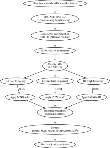
The goal of this experiment is to predict the DAX market index using a hybrid CEEMDAN-LSTM-BPNN model. The process begins with statistical tests for nonlinearity, followed by data decomposition using CEEMDAN, and then applying different models based on the decomposed data. A comparison is made between the hybrid model and various base models using different metrics across several train–test splits.

First, nonlinearity tests are conducted. The BDS test, developed by Brock, Dechert, and Scheinkman, is employed to detect the presence of nonlinearity in the time series data. Additionally, the augmented Dickey–Fuller (ADF) and Kwiatkowski–Phillips–Schmidt–Shin (KPSS) tests are used to verify stationarity, which is crucial for effective forecasting.

The data is then decomposed using the CEEMDAN technique. CEEMDAN provides a robust, adaptive method for handling nonstationary and nonlinear time series by breaking down the data into multiple IMFs, each representing different frequency components. This decomposition captures the different scales of variability and handles noise effectively through the adaptive noise mechanism embedded in the process.

After decomposition, the IMFs are classified based on variance and correlation analysis. HF IMFs are those with low variance and low correlation to the original series, while MF IMFs have moderate variance and correlation, and LF IMFs show high variance and high correlation. The HF and MF IMFs are modeled using LSTM networks, which are effective for time series data. In contrast, the LF IMFs are modeled using BPNNs. The results of these models are then ensembled by summing their outputs to create the final aggregated prediction.

The main model used in this experiment is the hybrid CEEMDAN-LSTM-BPNN model, which is compared to several base models. These include ARIMA, RNN, LSTM, GRU, BILSTM, BIGRU, BPNN, CEEMDAN-LSTM, CEEMDAN-GRU, CEEMDAN-BPNN, and CEEMDAN-GRU-BPNN. Each of these models is evaluated across different train–test splits (70/30, 80/20, and 90/10) for long-term, medium-term, and short-term predictions.

The performance of the models is evaluated using several metrics. The first metric is the RMSE, MAE, MAPE, SMAPE, R-squared, and RMSLE.

Data rescaling is critical to ensure that all input features are on a similar scale, which helps models like LSTM and BPNN converge more efficiently. In this experiment, min–max normalization is applied to scale the data to a range between 0 and 1. The formula for min–max normalization is

(32)

This equation represents the min–max normalization, where x^′ is the normalized value, x is the original value, and x_min and x_max are the minimum and maximum values of the original data, respectively.

To reverse this normalization and transform the normalized values x^′ back to the original scale, we use the following equation:

(33)

To ensure a fair comparison of model performance, all models were configured with the same hyperparameters. This consistency in hyperparameters ensures that any performance differences are due to the model architecture itself rather than variations in training settings.

Figure 7 shows the flowchart of the experimental design.

2.11. Parameter Settings

The choice of parameters for all models, including RNN, LSTM, GRU, BIGRU, BILSTM, and BPNN, is informed by commonly accepted practices in the literature and prior research to ensure consistent training and meaningful comparisons across models.

For the recurrent models (RNN, LSTM, GRU, BIGRU, BILSTM), the architecture follows a similar design. The models starts with input shapes for sequential data. The first layer has 128 units with a tanh activation function, followed by 64 units and then 32 units in the final recurrent layer. Dropout is applied after each layer, with a dropout rate of 0.2, a standard value to prevent overfitting. These parameters are commonly used to balance model complexity and generalization, as dropout helps regularize the network by randomly dropping some of the neurons during training, encouraging better generalization.

The learning rate is set to 0.001 for all models. This is a widely adopted choice for neural networks, particularly in time series prediction tasks, as it is small enough to allow the model to converge without instability. The Adam optimizer is chosen for its adaptability and efficiency, adjusting the learning rate based on each parameter’s gradient and momentum. This has been shown to be highly effective for training DL models on time series data. We adopted a batch size of 16 for all models. The loss function for all these models is MSE, which is standard for regression tasks like stock price prediction, as it penalizes large errors, making it useful in predicting financial time series where large deviations can significantly affect model performance.

For the BPNN, we used an architecture with 3 layers consisting of 128, 64, and 32 units. Dropout is also applied after each layer, and the same learning rate, batch size, activation function optimizer, and loss function are used. This design strikes a balance between avoiding overfitting and maintaining sufficient capacity for learning the data’s complexity. The choice of three layers is common in BPNN configurations, as it allows for enough depth to capture patterns without excessively increasing model complexity.

In addition to these parameter choices, training includes callbacks for early stopping and learning rate reduction. Early stopping monitors the validation loss and halts training if the loss does not improve for a certain number of epochs (patience), helping prevent overfitting and unnecessary computation. The ReduceLROnPlateau callback reduces the learning rate if the validation loss plateaus, further improving the training process by fine-tuning the learning rate as the model approaches convergence.

For the ARIMA model, we use AutoARIMA for automatic hyperparameter tuning, which searches through various combinations of model parameters (p, d, q) and selects the optimal configuration based on AIC (Akaike information criterion) or BIC (Bayesian information criterion). This allows us to identify the best-fitting ARIMA model for the time series data.

Python was used to analyze the data and implement all models.

2.12. Model Evaluation Metrics

To assess the performance of the predictive models, several evaluation metrics were employed, including RMSE, MAE, MAPE, coefficient of determination (R²), RMSLE, and SMAPE. These metrics offer comprehensive insights into the accuracy, precision, and robustness of the models in predicting the target variable.

The RMSE quantifies the average magnitude of prediction errors, penalizing larger deviations more significantly by squaring the errors:

(34)

Here, is the actual value, is the predicted value, and n is the number of observations.

RMSE is sensitive to outliers as it amplifies larger errors due to squaring.

The MAE provides the mean of the absolute differences between actual and predicted values, offering a linear scale of the average error:

(35)

MAE treats all errors uniformly by focusing on their magnitude, making it less influenced by outliers compared to RMSE.

MAPE expresses the prediction accuracy as a percentage of the actual values, emphasizing the relative size of the error:

(36)

While MAPE is intuitive, it can become unreliable when approaches zero, leading to inflated error values.

The R² metric, or the coefficient of determination, measures the proportion of variance in the actual values explained by the model:

(37)

where

is the mean of the actual values. An R² value near 1 signifies high predictive accuracy, while values close to 0 indicate poor model performance.

The RMSLE evaluates the logarithmic differences between actual and predicted values, reducing the impact of large errors when values are small:

(38)

RMSLE is particularly suited for tasks where underestimations are penalized more than overestimations. SMAPE provides a balanced percentage error by symmetrically accounting for both actual and predicted values:

(39)

SMAPE is designed to ensure fairness in error distribution between over- and underpredictions, offering a balanced view of prediction accuracy.

The performance of the proposed CEEMDAN-LSTM-BPNN model was evaluated across several key metrics, including RMSE, MAE, MAPE, SMAPE, and R-squared. To assess the effectiveness of the proposed model, the percentage improvement in performance over the benchmark models was computed for each of these metrics. The percentage improvement for each metric, M, was calculated using the formula:

(40)

where M_proposed represents the performance metric for the proposed model and M_benchmark is the performance metric for the benchmark model. This percentage improvement indicates how much better the proposed model performed compared to the benchmarks for each specific metric. To further validate the robustness of the model, the DM test was employed. The DM test [59] is designed to compare the predictive accuracy of two competing forecasting models. The null hypothesis of the DM test assumes that the two models have the same predictive accuracy, while the alternative hypothesis assumes that one model outperforms the other. In practice, forecast errors are computed for each time period t, and their squared differences are evaluated. The DM statistic is calculated by comparing the mean of these differences to the standard deviation, with a larger DM statistic indicating a significant difference in accuracy. If the DM statistic exceeds a critical value, the null hypothesis is rejected, indicating a significant difference in forecast accuracy between the models. The MCS test [60] is another method used to assess the relative performance of competing forecasting models. The MCS test is aimed at identifying a subset of models that perform similarly in terms of predictive accuracy, based on a chosen criterion. The null hypothesis of the MCS test asserts that all models in the comparison have similar predictive accuracy, while the alternative hypothesis suggests that there is a difference in performance among the models.

The MCS test evaluates the performance of multiple models by comparing their forecast errors, using statistical tests to identify models that are statistically indistinguishable in terms of their predictive accuracy. Models that are consistently superior across different error metrics are included in the confidence set, while models that perform poorly are excluded. If the null hypothesis is rejected, it indicates that some models are significantly worse than others, and further investigation is needed to identify the top-performing models. In both DM and MCS tests, MAE, MSE, and MAPE loss functions were used.

3. Results and Discussion

3.1. Statistical Analysis of the Data

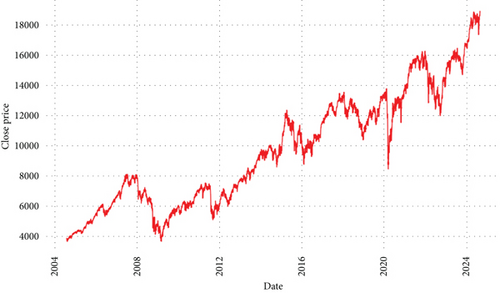
The market index daily closing price time series is displayed in Figure 8. Upon visual examination, we deduce a number of significant features pertaining to its nonstationarity and nonlinearity. The behavior of the data is rather nonlinear. The price series exhibits periods of notable ups and downs, most notably during the global financial crisis in 2008 and the COVID-19 pandemic in 2020. This implies that there is more to the data than a straightforward linear trend or model. Traditional linear modeling is unable to capture this behavior since the time series is dominated by complicated patterns that may be exponential or chaotic. Furthermore, it does not seem like the time series is stationary. There are visible trends and patterns over different periods, including an upward trend that dominates after each economic shock or crisis (e.g., 2009 and 2020). Furthermore, the volatility and variance of the series seem to change over time. For instance, the fluctuation around 2008 is sharper than those seen in other periods, indicating varying variance and mean across the timeline. This behavior violates the conditions for stationarity, where the mean and variance should be constant over time. Table 1 shows the summary statistics of the daily closing price.

Table 1. Summary statistics and test results for the time series.

Statistic/p value	Value
Mean	9725.6554
Variance	1.4509 × 10⁷
Standard deviation	3809.0265
Maximum	18,912.5703
Minimum	3646.9900
Kurtosis	−0.9474
Skewness	0.3447
ADF test statistic	−0.3558
ADF p value	0.9172
KPSS test statistic	10.7029
KPSS p value	0.0100
Jarque–Bera test statistic	291.9001
Jarque–Bera p value	p ≤ 0.001
Ljung–Box test statistic	50,388.6542
Ljung–Box p value	p ≤ 0.001

The summary statistics provide an overview of the time series characteristics. The mean value of the series is approximately 9725.6554, with a variance of 1.4509 × 10⁷, indicating substantial variability. The standard deviation (3809.0265) further supports this high variation. The maximum observed value in the series is 18,912.5703, while the minimum is 3646.9900, reflecting a wide range of fluctuations. The kurtosis of −0.9474 suggests that the distribution is flatter than normal, while the skewness of 0.3447 indicates slight positive asymmetry.

The results of the stationarity and normality tests provide critical insights. The ADF test, with a statistic of −0.3558 and a p value of 0.9172, suggests that the time series is nonstationary. The KPSS test corroborates this conclusion, with a high statistic of 10.7029 and a p value of 0.0100, leading to the rejection of the null hypothesis of stationarity. Furthermore, the Jarque–Bera test confirms that the series is not normally distributed (p ≤ 0.001), which aligns with the observed skewness and kurtosis.

The Ljung–Box test, with a test statistic value of 50,388.6542 and p ≤ 0.001, indicates strong evidence of autocorrelation in the time series. The extremely low p value suggests rejection of the null hypothesis of no autocorrelation, confirming the presence of long memory in the data. This implies that past values have a persistent influence on future values, requiring advanced modeling techniques for accurate forecasting.

As shown in Figure 9, significant autocorrelation is observed at multiple lags, indicating that past values have a substantial effect on the current values. This establishes the presence of long memory in the time series indicating a need for advanced modeling of the time series data.

The nonlinearity of the financial time series was further analyzed by conducting a BDS test on the residuals obtained from fitting an ARIMA model to the daily closing prices of the market index. The dataset was first divided into a training set (80%) and a testing set (20%). After fitting the ARIMA model to the training set, residuals and predicted values for the test set were computed. The BDS test was performed on these residuals to detect nonlinearity in the series.

The test was conducted across dimensions from 2 to 8, using an adjusted standard deviation (set at 70% of the test data’s standard deviation) as the threshold.

Table 2 presents the results of the BDS test. At a 5% significance level, all test statistics exhibit extremely low p values (p ≤ 0.001), leading to the rejection of the null hypothesis of linearity. This confirms that the time series data demonstrates significant nonlinearity, implying that traditional linear models may not be sufficient for accurate forecasting and necessitating the use of advanced nonlinear modeling techniques.

Table 2. BDS test results for dimensions 2–8.

Dimension	2	3	4	5	6	7	8
Test statistic	−12.3457	−11.7894	−13.5671	−14.2365	−12.9183	−15.0000	−8.7654
p value	p ≤ 0.001	p ≤ 0.001	p ≤ 0.001	p ≤ 0.001	p ≤ 0.001	p ≤ 0.001	p ≤ 0.001

Given that the series is nonnormal, nonstationary, and nonlinear, we applied the CEEMDAN method to decompose the series into IMFs and residuals for further analysis.

3.1.1. CEEMAN Decomposition Results

Figure 10 shows the IMFs and the residual derived from the CEEMDAN decomposition of the DAX market index time series. Each IMF corresponds to a different frequency component of the original signal, and the residual captures the long-term trend. The key observations can be summarized as follows: The first three IMFs (IMF 1 to IMF 3) contain HF oscillations with more noise-like behavior. These IMFs primarily capture short-term fluctuations, which may reflect market volatility or HF noise in the DAX market index. The amplitude of oscillations decreases gradually from IMF 1 to IMF 4.

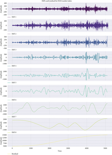
IMFs 4–6 exhibit midfrequency oscillations. These IMFs capture intermediate trends and cycles in the stock market, with more stable oscillations compared to the higher frequency components. The amplitude of these IMFs is larger than the higher-frequency components, suggesting their significance in capturing cyclical behavior. IMFs 7 and 8 and the residual are dominated by LF components. The residual captures the overall long-term trend in the data. These components reflect the persistent, slow-varying trends in the stock market, possibly related to macroeconomic factors. The higher-frequency IMFs are generally stable and have more variations, while the lower-frequency IMFs, especially the residual, are more nonstable and nonsmooth. This transition from HF to LF behavior is typical in CEEMDAN decompositions, which effectively separates different scales of variations in time series data. After applying CEEMDAN, the IMFs exhibit distinct characteristics at different frequencies. This is because CEEMDAN adaptively decomposes the signal into components that are locally narrow-band, thus providing better frequency separation.

The IMFs were grouped based on their variance proportion, Pearson correlation with the original series. The variance proportion of each IMF with respect to the original series can be used to identify which IMFs capture the most significant variations in the data. High variance proportions indicate that the IMF captures a substantial part of the original time series’ variability and vice versa is true.

Pearson correlation analysis and variance between the original time series and each IMF as shown in Table 3 help in understanding the relationship between the IMF and the original data. Higher correlations suggest that the IMF preserves more of the structure of the original series.

Table 3. Correlation and variance results of decomposed DAX market index IMFs.

Group	IMF	Correlation with original	Variance percentage (%)
High frequency (HF)	IMF 1	0.020010	0.022201
	IMF 2	0.012795	0.022231
	IMF 3	0.044865	0.057346

Medium frequency (MF)	IMF 4	0.052149	0.203753
	IMF 5	0.080426	0.543886
	IMF 6	0.130854	1.022644

Low frequency (LF)	IMF 7	0.219252	2.338082
	IMF 8	0.155374	3.146278
	Residual	0.961001	92.643579

The plot in Figure 11 shows the decomposition of the original price series into its HF, MF, and LF components using different IMFs. Here is a breakdown of how to interpret and utilize the graph in relation to the LSTM and BPNN model.

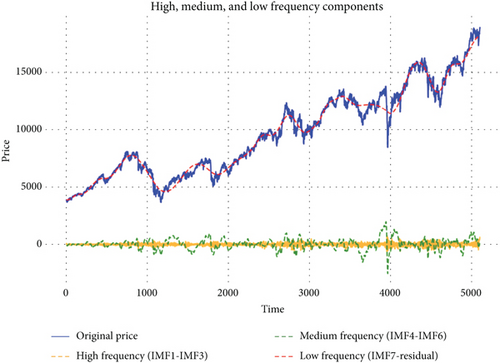
Original price (in blue): This represents the actual price series you are trying to model or forecast.

HF components (IMF1–IMF3): The yellow dashed line represents the sum of the first three IMFs, which are the highest frequency components. These components tend to capture short-term oscillations and are modeled using LSTM for their temporal dependencies.

MF components (IMF4–IMF6): The green dashed line represents the MF components, capturing intermediate trends in the price series. This is also modeled using LSTM.

LF components (IMF7–IMF8 + residual): The red dashed line represents the LF components along with the residual, which captures long-term trends. These are modeled using a BPNN, as they generally represent more stable and slowly varying components of the price. Let the IMFs be denoted as IMF₁, IMF₂, ⋯, IMF_n, where n is the total number of IMFs, and the residual is also treated as an IMF. The final prediction

can be represented as the sum of the predictions from each group:

(41)

where

is the prediction for the i-th IMF.

We divide the IMFs into three groups based on their frequency characteristics:

-
HF:

(42)

-
MF:

(43)

-
LF:

(44)

For the HF and MF components, the prediction is modeled using an LSTM:

(45)

(46)

For the LF components, the prediction is modeled using a BPNN:

(47)

The final ensemble prediction is obtained by summing the predictions from each frequency group:

(48)

3.2. Empirical Results

In this section, we present the empirical findings from applying the proposed CEEMDAN-LSTM-BPNN model and compare its performance against several benchmark models. To evaluate the models, we used different training and testing splits, specifically 70:30, 80:20, and 90:10, to assess the models’ ability to generalize across various data ranges. The benchmark models used for comparison include the standard ARIMA, RNN, LSTM, GRU, BIGRU, BILSTM, and BPNN, alongside the actual ground truth. Additionally, we incorporated enhanced models such as CEEMDAN-GRU, CEEMDAN-LSTM, CEEMDAN-BPNN, and CEEMDAN-GRU-BPNN to further assess the impact of using CEEMDAN decomposition before applying predictive models.

The results are evaluated by analyzing the model performances across these different training/testing splits, which allowed us to examine the models’ robustness and accuracy over both short-term and long-term forecast horizons. The training and forecast results for each time series are displayed in corresponding figures, where each model configuration’s performance is visualized. These plots offer insights into how the CEEMDAN-based models perform compared to traditional DL and neural network models.

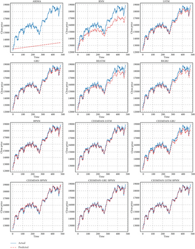
Figure 12 presents the time series predictions for actual prices compared to various models, utilizing a 70:30 training and testing split. Each subplot showcases the performance of different forecasting models against the actual price series.

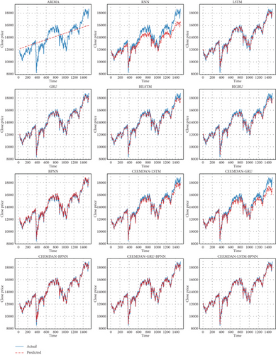
The blue line represents the actual prices, while the dashed lines in varying colors denote the predictions made by each model. This visualization allows for a clear comparison of how well each model captures the trends and fluctuations of the actual price series.

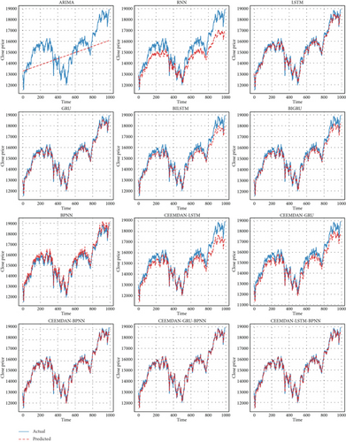
The 70:30 split implies that 70% of the data was used for training the models, while the remaining 30% was reserved for testing their predictive performance. This approach helps assess the models’ robustness and generalization ability on unseen data, providing insights into their effectiveness in forecasting price movements in time series data. Similarly, Figure 13 shows the time series predictions for actual prices compared to various models, utilizing an 80:20 training and testing split, and Figure 14 shows time series predictions for actual prices compared to various models, utilizing a 90:10 training and testing split. The benchmark models, including ARIMA, RNN, LSTM, GRU, BIGRU, BILSTM, and BPNN, exhibit varying degrees of alignment with the actual price series across the three training–testing splits. As shown in Figures 12, 13, and 14, these models capture general price trends but struggle with finer fluctuations and sudden market shifts. While DL models like LSTM and GRU improve over traditional statistical approaches such as ARIMA, their standalone performance remains limited in fully capturing the complexities of financial time series data. Across all three training–testing splits, the proposed CEEMDAN-LSTM-BPNN model consistently outperforms benchmark models, demonstrating superior alignment with actual price movements.

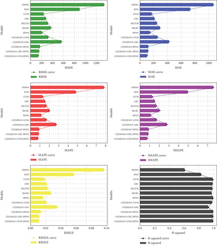
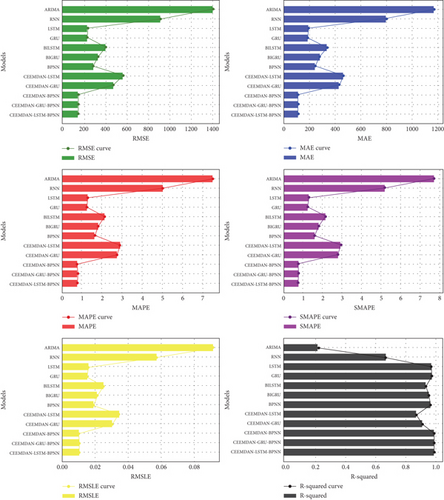
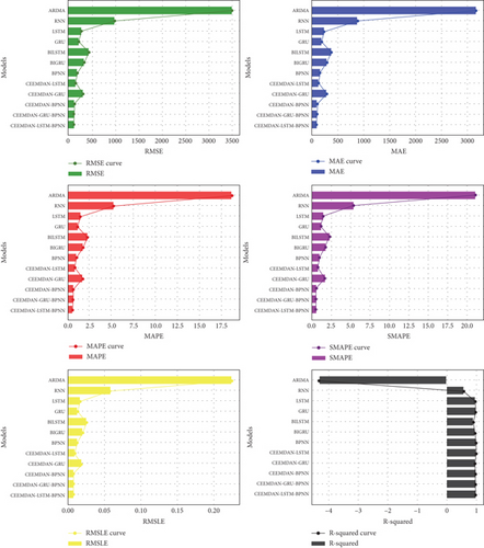
The performance evaluation of different forecasting models across three train–test splits (70:30, 80:20, and 90:10) reveals distinct trends in predictive accuracy and robustness. The proposed CEEMDAN-LSTM-BPNN model consistently outperformed all benchmarks across all splits, demonstrating its superior forecasting ability. The six evaluation metrics considered include MAE, RMSE, MAPE, SMAPE, RMSLE, and R-squared, where lower values indicate better performance, except for R-squared, where higher values are preferred. The standalone benchmarks, including ARIMA, RNN, LSTM, GRU, BILSTM, BIGRU, and BPNN, and other hybrid models, such as CEEMDAN-LSTM, CEEMDAN-GRU, CEEMDAN-BPNN, and CEEMDAN-GRU-BPNN, exhibited varying degrees of performance, with ARIMA performing the worst in all cases due to its limited capability in capturing nonstationarity and nonlinear dependencies. It is important to note that GRU, LSTM, and BPNN were considered as prediction models for integration with CEEMDAN since they showed superior performance for the undecomposed time series.

As shown on Table 4, for the 70:30 split, the CEEMDAN-LSTM-BPNN model achieved MAE of 143.2891, RMSE of 106.7459, MAPE of 0.7760, SMAPE of 0.7768, RMSLE of 0.0110, and R-squared of 0.9954, making it the most effective among all models. In contrast, ARIMA exhibited significantly poorer performance with MAE of 1321.4853, RMSE of 1066.2593, MAPE of 7.8115, SMAPE of 7.5906, RMSLE of 0.0965, and R-squared of 0.6081. Standalone models, such as BPNN, GRU, and LSTM, performed relatively well but failed to surpass this hybrid decomposition approach, emphasizing the advantage of CEEMDAN in extracting meaningful time series components.

Table 4. Performance metrics of different models across various train–test splits (70:30, 80:20, and 90:10). Each model’s performance is evaluated using metrics such as MAE, RMSE, MAPE, SMAPE, RMSLE, and R-squared with lower values indicating better performance. The CEEMDAN-LSTM-BPNN model consistently demonstrates superior performance across different splits, showcasing its effectiveness in forecasting tasks.

Model	MAE	RMSE	MAPE	SMAPE	RMSLE	R -squared
70/30 split
ARIMA	1321.4853	1066.2593	7.8115	7.5906	0.0965	0.6081
RNN	881.5902	728.5326	4.7895	4.9363	0.0571	0.8256
LSTM	236.9373	174.9211	1.2878	1.2839	0.0188	0.9874
GRU	276.3742	210.3549	1.5259	1.5290	0.0212	0.9829
BILSTM	311.0839	241.7233	1.6969	1.7018	0.0226	0.9783
BIGRU	363.4021	284.5164	2.0240	2.0316	0.0272	0.9704
BPNN	210.2672	150.7960	1.1176	1.1089	0.0164	0.9901
CEEMDAN-LSTM	320.7262	255.8260	1.7047	1.7235	0.0208	0.9769
CEEMDAN-GRU	557.5576	422.1375	2.7306	2.7864	0.0348	0.9302
CEEMDAN-BPNN	168.1379	120.5389	0.8900	0.8914	0.0136	0.9937
CEEMDAN-GRU-BPNN	152.6728	117.2044	0.8389	0.8408	0.0114	0.9948
CEEMDAN-LSTM-BPNN	143.2891	106.7459	0.7760	0.7768	0.0110	0.9954

80/20 split
ARIMA	1401.3706	1172.1456	7.5074	7.7089	0.0912	0.2319
RNN	916.1111	802.2986	5.0181	5.1742	0.0573	0.6717
LSTM	239.1977	195.3599	1.2881	1.2924	0.0160	0.9776
GRU	232.2502	189.7146	1.2469	1.2529	0.0155	0.9789
BILSTM	402.9920	337.7513	2.1351	2.1606	0.0251	0.9365
BIGRU	333.6762	281.9086	1.8063	1.8229	0.0213	0.9565
BPNN	290.3984	246.5575	1.6236	1.6061	0.0191	0.9670
CEEMDAN-LSTM	566.2859	464.0749	2.8802	2.9376	0.0345	0.8746
CEEMDAN-GRU	475.6489	432.1323	2.7575	2.8023	0.0303	0.9115
CEEMDAN-BPNN	150.3645	114.1812	0.7622	0.7645	0.0103	0.9912
CEEMDAN-GRU-BPNN	150.7501	114.3783	0.7710	0.7724	0.0105	0.9911
CEEMDAN-LSTM-BPNN	149.5960	114.1334	0.7628	0.7651	0.0103	0.9912

90/10 split
ARIMA	3393.9263	3162.3782	18.9104	21.1235	0.2245	−4.3077
RNN	965.8831	884.2548	5.2825	5.4460	0.0582	0.5701
LSTM	279.5752	243.8834	1.4833	1.4968	0.0171	0.9640
GRU	223.1949	190.1714	1.1619	1.1700	0.0137	0.9770
BILSTM	435.3062	378.2306	2.2553	2.2875	0.0257	0.9127
BIGRU	339.8085	293.7352	1.7760	1.7955	0.0205	0.9468
BPNN	195.4164	161.1688	0.9950	1.0010	0.0122	0.9824
CEEMDAN-LSTM	161.5198	133.1521	0.8107	0.8148	0.0098	0.9880
CEEMDAN-GRU	311.6527	284.5629	1.7260	1.7435	0.0188	0.9552
CEEMDAN-BPNN	134.2087	105.1037	0.6501	0.6474	0.0083	0.9917
CEEMDAN-GRU-BPNN	125.0369	97.0205	0.5949	0.5966	0.0076	0.9928
CEEMDAN-LSTM-BPNN	118.1318	91.1118	0.5628	0.5638	0.0073	0.9936

Note: Performance metrics of different models across various train–test splits (70:30, 80:20, and 90:10). Each model’s performance is evaluated using metrics such as MAE, RMSE, MAPE, SMAPE, RMSLE, and R-squared with lower values indicating better performance. The CEEMDAN-LSTM-BPNN model consistently demonstrates superior performance across different splits as shown by the bold values, showcasing its effectiveness in forecasting tasks.

A similar pattern emerged in the 80:20 split, where CEEMDAN-LSTM-BPNN again exhibited the best results with MAE of 149.5960, RMSE of 114.1334, MAPE of 0.7628, SMAPE of 0.7651, RMSLE of 0.0103, and R-squared of 0.9912. The worst-performing model, ARIMA, resulted in MAE of 1401.3706, RMSE of 1172.1456, MAPE of 7.5074, SMAPE of 7.7089, RMSLE of 0.0912, and R-squared of only 0.2319, highlighting its inefficiency in capturing complex temporal dependencies. Notably, the CEEMDAN-GRU-BPNN model, despite incorporating decomposition and neural networks, did not outperform the proposed approach, suggesting that the combination of LSTM with BPNN adds critical value.

In the 90:10 split, the CEEMDAN-LSTM-BPNN model continued to demonstrate superior results with MAE of 118.1318, RMSE of 91.1118, MAPE of 0.5628, SMAPE of 0.5638, RMSLE of 0.0073, and R-squared of 0.9936. ARIMA was again the worst performer, with MAE of 3393.9263, RMSE of 3162.3782, MAPE of 18.9104, SMAPE of 21.1235, RMSLE of 0.2245, and R-squared of −4.3077, signifying its complete failure in this context.

An interesting observation is that CEEMDAN-GRU and CEEMDAN-LSTM models did not perform well. This is attributed to the limitation of GRU and LSTM in effectively modeling LF trend component, a task better handled by BPNN. The integration of BPNN in the proposed model thus provides a crucial advantage by capturing these long-term dependencies, enhancing overall predictive stability.

These findings suggest that for effective financial time series forecasting, a hybrid decomposition–ensemble approach utilizing CEEMDAN, LSTM, and BPNN should be taken into consideration. The combination ensures that HF variations and MF variations are modeled by the LSTM networks while LF trends are captured by BPNN, leading to robust overall performance.

Figure 15 presents the evaluation metrics for the 70:30 train–test split, while Figure 16 illustrates the metrics for the 80:20 split. Similarly, Figure 17 displays the performance metrics for the 90:10 split, enabling a comparative analysis across different data partitions.

To visually validate these findings, scatter plots of predicted versus actual values for each train–test split are presented for the proposed model and the benchmark models. Figure 18 illustrates the 70:30 split, Figure 19 corresponds to the 80:20 split, and Figure 20 represents the 90:10 split. Each scatter plot aligns the predictions of the proposed model against the true values, confirming its effectiveness in capturing time series patterns accurately. It is noted that the proposed model demonstrates strong alignment with actual values, outperforming benchmark model in all data splits.

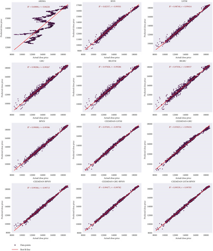
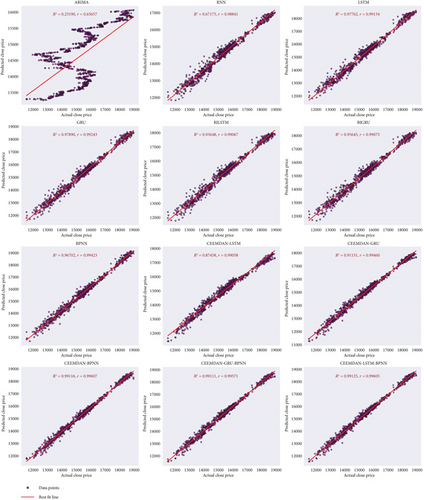
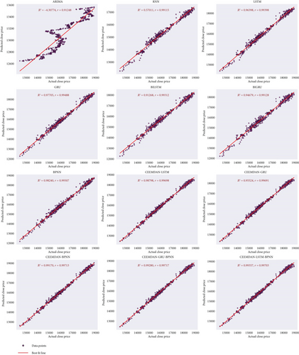
These visualizations further support the quantitative results, demonstrating that the CEEMDAN-LSTM-BPNN model maintains high accuracy across different data splits.

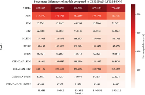
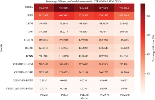
The percentage improvement of the proposed CEEMDAN-LSTM-BPNN model over the benchmark models is visualized through heatmaps. Darker colors indicate a higher percentage of improvement, signifying better performance of the proposed model, while lighter colors indicate relatively lower improvements. The analysis is based on the first five metrics: PRMSE, PMAE, PMAPE, PSMAPE, and PRMSLE.

As shown in Figure 21, for the 70:30 split, the proposed model exhibited significant improvements compared to standalone models, particularly ARIMA, which displayed the highest percentage improvement metrics (PRMSE: 822.25%, PMAE: 898.88%, PMAPE: 906.70%, PSMAPE: 877.21%, PRMSLE: 779.65%). In contrast, the proposed CEEMDAN-LSTM-BPNN model consistently outperformed the benchmark CEEMDAN-GRU-BPNN which showed the lowest improvement metrics (PRMSE: 6.55%, PMAE: 9.80%, PMAPE: 8.11%, PSMAPE: 8.25%, PRMSLE: 3.49%), demonstrating its effectiveness in reducing forecasting errors. Notably, there is significant improvements compared to other benchmark models too.

As shown in Figure 22, in the 80:20 split, the proposed model continued to demonstrate superior performance over the benchmark CEEMDAN-GRU-BPNN (PRMSE: 0.77%, PMAE: 0.21%, PMAPE: 1.08%, PSMAPE: 0.96%, PRMSLE: 1.67%). The improvement is most evident when compared to ARIMA and RNN, where the percentage differences are substantial. Other models also show significant improvement too.

As shown in Figure 23, for the 90:10 split, the overall percentage improvements highlight the stability and efficiency of the proposed model even with a reduced test dataset. ARIMA again exhibited the highest improvement values (PRMSE: 2772.99%, PMAE: 3370.88%, PMAPE: 3260.08%, PSMAPE: 3646.75%, PRMSLE: 2983.35%), whereas the CEEMDAN-GRU-BPNN benchmark showed significantly lower values (PRMSE: 5.85%, PMAE: 6.49%, PMAPE: 5.71%, PSMAPE: 5.82%, PRMSLE: 5.03%). The improvement is also evident when compared to other benchmark models.

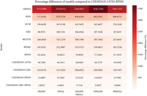
Across all train–test splits, the CEEMDAN-LSTM-BPNN model demonstrates consistent and substantial improvements over the benchmark models. The most significant improvements are observed against ARIMA and RNN, confirming the advantage of the hybrid model over purely standalone methods. The percentage improvements across different metrics affirm the effectiveness of CEEMDAN in decomposition, combined with LSTM and BPNN for capturing long-term dependencies and nonlinearity in financial time series. The model’s stability across different splits suggests its suitability for robust market index forecasting.

The percentage improvement metric, while useful for assessing relative gains in predictive performance, has inherent limitations as it does not account for statistical significance and is sensitive to variations in the magnitude of errors. Small absolute differences in loss functions can lead to disproportionately high percentage changes, making direct comparisons across models less reliable. Additionally, percentage improvement does not reflect the consistency of a model’s advantage across different forecast horizons, which is crucial in financial forecasting. To address these issues, the DM test was employed to formally evaluate whether the differences in forecast accuracy between the proposed CEEMDAN-LSTM-BPNN model and its benchmarks are statistically significant (Table 5).

Table 5. Diebold–Mariano (DM) test results comparing the CEEMDAN-LSTM-BPNN model with benchmark models across three train–test splits (70:30, 80:20, and 90:10). The negative values indicate that the proposed model outperforms the benchmarks in terms of MAE, MSE, and MAPE. All table values are set to 4 decimal places.

Model	70:30			80:20			90:10
Model	MAE	MSE	MAPE	MAE	MSE	MAPE	MAE	MSE	MAPE
ARIMA	−48.4378 ^∗∗∗	−26.8083 ^∗∗∗	−42.0959 ^∗∗∗	−42.5522 ^∗∗∗	−29.5855 ^∗∗∗	−43.7952 ^∗∗∗	−54.7133 ^∗∗∗	−31.5699 ^∗∗∗	−66.5364 ^∗∗∗
RNN	−48.1911 ^∗∗∗	−30.9643 ^∗∗∗	−54.4941 ^∗∗∗	−47.1484 ^∗∗∗	−29.9733 ^∗∗∗	−52.5357 ^∗∗∗	−44.6527 ^∗∗∗	−27.1140 ^∗∗∗	−51.7473 ^∗∗∗
LSTM	−19.2103 ^∗∗∗	−10.1848 ^∗∗∗	−16.9667 ^∗∗∗	−18.8494 ^∗∗∗	−13.7421 ^∗∗∗	−17.6532 ^∗∗∗	−25.7236 ^∗∗∗	−20.3148 ^∗∗∗	−26.0728 ^∗∗∗
GRU	−25.3083 ^∗∗∗	−14.7142 ^∗∗∗	−22.9198 ^∗∗∗	−18.9301 ^∗∗∗	−14.6017 ^∗∗∗	−17.7606 ^∗∗∗	−21.1244 ^∗∗∗	−17.0124 ^∗∗∗	−21.3272 ^∗∗∗
BILSTM	−29.5135 ^∗∗∗	−17.3807 ^∗∗∗	−26.9517 ^∗∗∗	−31.0171 ^∗∗∗	−22.5682 ^∗∗∗	−31.8597 ^∗∗∗	−29.6582 ^∗∗∗	−20.7975 ^∗∗∗	−31.6687 ^∗∗∗
BIGRU	−32.8034 ^∗∗∗	−17.2759 ^∗∗∗	−29.1640 ^∗∗∗	−29.1487 ^∗∗∗	−22.5055 ^∗∗∗	−28.8646 ^∗∗∗	−27.2622 ^∗∗∗	−20.0278 ^∗∗∗	−27.9849 ^∗∗∗
BPNN	−12.7007 ^∗∗∗	−9.6306 ^∗∗∗	−12.8175 ^∗∗∗	−23.2074 ^∗∗∗	−18.2531 ^∗∗∗	−22.5985 ^∗∗∗	−16.0387 ^∗∗∗	−13.0291 ^∗∗∗	−16.1494 ^∗∗∗
CEEMDAN-LSTM	−32.0530 ^∗∗∗	−24.0968 ^∗∗∗	−33.4543 ^∗∗∗	−33.6098 ^∗∗∗	−22.0362 ^∗∗∗	−36.3986 ^∗∗∗	−13.9056 ^∗∗∗	−13.1303 ^∗∗∗	−13.9131 ^∗∗∗
CEEMDAN-GRU	−33.9654 ^∗∗∗	−22.5231 ^∗∗∗	−36.7148 ^∗∗∗	−49.2342 ^∗∗∗	−34.3447 ^∗∗∗	−53.0737 ^∗∗∗	−33.7701 ^∗∗∗	−25.1760 ^∗∗∗	−35.1388 ^∗∗∗
CEEMDAN-BPNN	−6.2093 ^∗∗∗	−4.4622 ^∗∗∗	−5.6346 ^∗∗∗	−0.0245 ^∗	−0.2749 ^∗	0.0407 ^∗	−3.3425 ^∗∗∗	−3.1931 ^∗∗∗	−3.4254 ^∗∗∗
CEEMDAN-GRU-BPNN	−11.0153 ^∗∗∗	−8.7750 ^∗∗∗	−9.4612 ^∗∗∗	−0.1705 ^∗	−0.7340 ^∗	−0.8708 ^∗	−3.5575 ^∗∗∗	−3.9381 ^∗∗∗	−3.2187 ^∗∗∗

Note: Statistical significance is denoted by ^∗∗∗ (1% level), ^∗∗ (5% level), and ^∗ (10% level).

The DM test was conducted under the null hypothesis that there is no significant difference in forecast errors between the CEEMDAN-LSTM-BPNN model and each benchmark model. The alternative hypothesis posits that the proposed model yields significantly lower forecast errors. The results indicate that for all benchmark models, the CEEMDAN-LSTM-BPNN model consistently outperforms them, with negative DM statistics across all train–test splits. The statistical significance at the 1% level (denoted by ^∗∗∗) in most cases confirms that the improvements observed are not due to random chance, reinforcing the robustness of the proposed approach. However, at the 80:20 split, the CEEMDAN-BPNN and CEEMDAN-GRU-BPNN configurations exhibit marginal improvements with lower significance levels (), suggesting that in some cases, the advantage may be less pronounced.

Across different train–test splits and loss functions, the results highlight the superiority of DL-based hybrid models over traditional statistical and standalone DL models. Classical models like ARIMA show the weakest performance, with the highest DM values indicating significant inferiority compared to CEEMDAN-LSTM-BPNN.

The MCS test was conducted using the parameters, window size, and bootstrap iterations. The bootstrap resampling process was applied to the loss differential data to iteratively estimate the distribution of the test statistics, allowing the identification of models belonging to the superior set with a confidence level of 90%. The results show in Table 6 that for the 70/30 split, only the CEEMDAN-LSTM-BPNN model consistently remained within the MCS, achieving a p value of 1.0000 across all evaluation metrics. Conversely, traditional models such as ARIMA, RNN, LSTM, GRU, and BPNN were excluded from the superior set, as evidenced by their near-zero p values. This pattern suggests that the proposed CEEMDAN-LSTM-BPNN hybrid model significantly outperforms their standalone counterparts and other hybrids in financial time series forecasting.

Table 6. p values for model confidence set (MCS) test across different training splits (70/30, 80/20, and 90/10). The MCS test evaluates whether a model belongs to the set of superior models at a confidence level of 90%. The null hypothesis (H₀) states that the model’s predictive performance is statistically equivalent to the best-performing model in the set. A p value close to 1 indicates strong evidence that the model is among the superior models, whereas a value near 0 suggests rejection from the MCS. All p values greater than 0.1 are underlined.

Model	(R) MSE	(SQ) MSE	(R) MAE	(SQ) MAE	(R) MAPE	(SQ) MAPE
70/30 split
ARIMA	0.0000	0.0000	0.0000	0.0000	0.0000	0.0000
RNN	0.0000	0.0000	0.0000	0.0000	0.0000	0.0000
LSTM	0.0000	0.0000	0.0000	0.0000	0.0000	0.0000
GRU	0.0000	0.0000	0.0000	0.0000	0.0000	0.0000
BILSTM	0.0000	0.0000	0.0000	0.0000	0.0000	0.0000
BIGRU	0.0000	0.0000	0.0000	0.0000	0.0000	0.0000
BPNN	0.0000	0.0000	0.0000	0.0000	0.0000	0.0000
CEEMDAN-LSTM	0.0000	0.0000	0.0000	0.0000	0.0000	0.0000
CEEMDAN-GRU	0.0000	0.0000	0.0000	0.0000	0.0000	0.0000
CEEMDAN-BPNN	0.0000	0.0000	0.0000	0.0000	0.0000	0.0000
CEEMDAN-GRU-BPNN	0.0000	0.0000	0.0000	0.0000	0.0000	0.0000
CEEMDAN-LSTM-BPNN	1.0000	1.0000	1.0000	1.0000	1.0000	1.0000

80/20 split
ARIMA	0.0000	0.0000	0.0000	0.0000	0.0000	0.0000
RNN	0.0000	0.0000	0.0000	0.0000	0.0000	0.0000
LSTM	0.0000	0.0000	0.0000	0.0000	0.0000	0.0000
GRU	0.0000	0.0000	0.0000	0.0000	0.0000	0.0000
BILSTM	0.0000	0.0000	0.0000	0.0000	0.0000	0.0000
BIGRU	0.0000	0.0000	0.0000	0.0000	0.0000	0.0000
BPNN	0.0000	0.0000	0.0000	0.0000	0.0000	0.0000
CEEMDAN-LSTM	0.0000	0.0000	0.0000	0.0000	0.0000	0.0000
CEEMDAN-GRU	0.0000	0.0000	0.0000	0.0000	0.0000	0.0000
CEEMDAN-BPNN	0.8438	0.8860	0.9941	0.9934	0.8161	0.8300
CEEMDAN-GRU-BPNN	0.8438	0.8860	0.9941	0.9934	0.9750	0.9752
CEEMDAN-LSTM-BPNN	1.0000	1.0000	1.0000	1.0000	1.0000	1.0000

90/10 split
ARIMA	0.0000	0.0000	0.0000	0.0000	0.0000	0.0000
RNN	0.0000	0.0000	0.0000	0.0000	0.0000	0.0000
LSTM	0.0000	0.0000	0.0000	0.0000	0.0000	0.0000
GRU	0.0000	0.0000	0.0000	0.0000	0.0000	0.0000
BILSTM	0.0000	0.0000	0.0000	0.0000	0.0000	0.0000
BIGRU	0.0000	0.0000	0.0000	0.0000	0.0000	0.0000
BPNN	0.0000	0.0000	0.0000	0.0000	0.0000	0.0000
CEEMDAN-LSTM	0.0000	0.0000	0.0000	0.0000	0.0000	0.0000
CEEMDAN-GRU	0.0000	0.0000	0.0000	0.0000	0.0000	0.0000
CEEMDAN-BPNN	0.0011	0.0021	0.0029	0.0014	0.0046	0.0027
CEEMDAN-GRU-BPNN	0.0011	0.0021	0.0029	0.0014	0.0046	0.0027
CEEMDAN-LSTM-BPNN	1.0000	1.0000	1.0000	1.0000	1.0000	1.0000

Note: Performance metrics of different models across various train–test splits (70:30, 80:20, and 90:10). Each model’s performance is evaluated using metrics such as MAE, RMSE, MAPE, SMAPE, RMSLE, and R-squared with lower values indicating better performance. The CEEMDAN-LSTM-BPNN model consistently demonstrates superior performance across different splits as shown by the bold values, showcasing its effectiveness in forecasting tasks.

For the 80/20 split, the findings remain consistent, with the CEEMDAN-LSTM-BPNN model maintaining its inclusion in the MCS, reaffirming its robustness. However, a notable difference is the emergence of CEEMDAN-BPNN and CEEMDAN-GRU-BPNN with moderately high p values, particularly in MAPE-based metrics, where they achieved values above 0.1 This indicates that, while these models exhibit competitive performance, they do not consistently reach the level of the superior CEEMDAN-LSTM-BPNN. The results also suggest that as the training data proportion increases, some hybrid models begin to demonstrate stronger performance, likely benefiting from improved generalization and stability in loss estimation. The 90/10 split further supports these conclusions, with CEEMDAN-LSTM-BPNN remaining the dominant model across all metrics. The implications of these results are significant for financial forecasting applications. The superiority of CEEMDAN-LSTM-BPNN hybrid model demonstrates the effectiveness of signal decomposition in capturing nonstationary and nonlinear components of financial data. The findings also highlight that while simpler models may perform reasonably well with sufficient data, the decomposition–ensemble approach provides a clear advantage in ensuring robustness and predictive accuracy.

4. Conclusion

In conclusion, this study has demonstrated the efficacy of the CEEMDAN-LSTM-BPNN model for forecasting the DAX market index, effectively addressing the complexities inherent in financial time series data, particularly the nonlinearity and nonstationarity. By employing the CEEMDAN decomposition technique, the model successfully decomposed the financial time series data into LF, MF, and HF components. The grouping of these components was achieved through correlation and variance analysis, which provided a more effective way to classify and manage the different time scales in the data. The integration of advanced neural network architectures, namely, LSTM and BPNN, resulted in a robust forecasting mechanism that outperformed traditional models and other benchmark models across various performance metrics, such as RMSE, MAE, MAPE, SMAPE, RMSLE, and R-squared. These results underscore the model’s adaptability and high performance across different forecast horizons, showing its potential for real-world financial applications.

The study also highlighted the importance of considering both statistical and ML methods for addressing the challenges posed by financial time series data. The CEEMDAN-LSTM-BPNN hybrid model provided notable improvements over simpler models, which often fail to capture the complex patterns in the data. The extensive evaluation through both direct testing and the MCS test has shown the proposed model’s superior forecasting ability.

5. Future Studies

In future studies, several avenues of research could extend and refine the current work. One major limitation of this study was the use of a single dataset, the DAX market index. A natural next step would be to apply the CEEMDAN-LSTM-BPNN model to a broader range of datasets, including emerging markets, commodities, and even cryptocurrency data. This would help assess the model’s robustness and versatility across different market conditions and whether it can maintain its high performance across various asset classes and financial environments.

Moreover, future work could explore the use of multistep forecasting techniques, which would allow for long-term predictions rather than focusing on short-term forecasting. This could involve adapting the current model architecture or integrating more advanced neural networks like transformers or attention mechanisms, which have been shown to excel in sequence prediction tasks. Investigating other decomposition techniques such as VMD to further decompose the HF component could also further improve the accuracy and stability of the model.

Finally, the consideration of other factors influencing stock price movements could greatly enhance the model’s predictive capabilities. Incorporating external data sources such as macroeconomic indicators, geopolitical events, or even sentiment analysis from news sources could provide additional insights into market behavior, leading to more informed and accurate forecasts. This would also require careful attention to parameter fine-tuning, as the optimal configuration of the model is crucial to achieving the best results. Exploring these additional dimensions of forecasting will pave the way for more comprehensive and robust financial prediction systems in the future.

Nomenclature

ARIMA: autoregressive integrated moving average
BPNN: backpropagation neural network
CEEMDAN: complete ensemble empirical mode decomposition with adaptive noise
EEMD: ensemble empirical mode decomposition
EMD: empirical mode decomposition
GARCH: generalized autoregressive conditional heteroskedasticity
GRU: gated recurrent unit
HF: high frequency
IMFs: intrinsic mode functions
LF: low frequency
LSTM: long short-term memory
MAE: mean absolute error
MAPE: mean absolute percentage error
MF: medium frequency
RMSE: root mean squared error
RMSLE: root mean squared logarithmic error
SMAPE: symmetric mean absolute percentage error
VMD: variational mode decomposition

Consent

The authors have nothing to report.

Conflicts of Interest

The authors declare no conflicts of interest.

Author Contributions

John Kamwele Mutinda: writing–original draft, writing–review, editing, software, methodology, data curation, and conceptualization. Abebe Geletu: writing–review and supervision.

Funding

No funding was received for this research.

Open Research

Data Availability Statement

The data are not publicly available due to privacy or ethical restrictions.

References

1 Shumway R. H. and Stoffer D. S., Time Series Analysis and Its Applications, 2000, 3, Springer, https://doi.org/10.1007/978-1-4757-3261-0.
10.1007/978-1-4757-3261-0
Google Scholar
2 Fuller W. A., Introduction to Statistical Time Series, 2009, John Wiley & Sons.
Google Scholar
3 Müller U. K. and Watson M. W., Low-Frequency Econometrics, 2015, Technical report, National Bureau of Economic Research.
10.3386/w21564
Google Scholar
4 Kim Y. S., Rachev S. T., Bianchi M. L., Mitov I., and Fabozzi F. J., Time series analysis for financial market meltdowns, Journal of Banking & Finance. (2011) 35, no. 8, 1879–1891, https://doi.org/10.1016/j.jbankfin.2010.12.007, 2-s2.0-79957605668.
10.1016/j.jbankfin.2010.12.007
Web of Science® Google Scholar
5 Sezer O. B., Gudelek M. U., and Ozbayoglu A. M., Financial time series forecasting with deep learning: a systematic literature review: 2005–2019, Applied Soft Computing. (2020) 90, 106181, https://doi.org/10.1016/j.asoc.2020.106181.
10.1016/j.asoc.2020.106181
Web of Science® Google Scholar
6 Mehtab S. and Sen J., A time series analysis-based stock price prediction using machine learning and deep learning models, International Journal of Business Forecasting and Marketing Intelligence. (2020) 6, no. 4, 272–335, https://doi.org/10.1504/IJBFMI.2020.115691.
10.1504/IJBFMI.2020.115691
Google Scholar
7 Mehtab S. and Sen J., Stock price prediction using convolutional neural networks on a multivariate timeseries, 2020, https://arxiv.org/abs/2001.09769.
Google Scholar
8 Elliot A. and Hsu C. H., Time series prediction: predicting stock price, https://arxiv.org/abs/1710.05751.
Google Scholar
9 Zhao C., Hu P., Liu X., Lan X., and Zhang H., Stock market analysis using time series relational models for stock price prediction, Mathematics. (2023) 11, no. 5, https://doi.org/10.3390/math11051130.
10.3390/math11051130
Web of Science® Google Scholar
10 Ali M., Khan D. M., Aamir M., Ali A., and Ahmad Z., Predicting the direction movement of financial time series using artificial neural network and support vector machine, Complexity. (2021) 2021, 13, 2906463, https://doi.org/10.1155/2021/2906463.
10.1155/2021/2906463
Web of Science® Google Scholar
11 Ashok Kumar D. and Murugan S., Performance analysis of Indian stock market index using neural network time series model, 2013 International Conference on Pattern Recognition, Informatics and Mobile Engineering, February 2013, Salem, India, 72–78, https://doi.org/10.1109/ICPRIME.2013.6496450, 2-s2.0-84876773429.
10.1109/ICPRIME.2013.6496450
Google Scholar
12 Song D., Chung Baek A. M., and Kim N., Forecasting stock market indices using padding-based Fourier transform denoising and time series deep learning models, IEEE Access. (2021) 9, 83786–83796, https://doi.org/10.1109/ACCESS.2021.3086537.
10.1109/ACCESS.2021.3086537
Web of Science® Google Scholar
13 Leu Y., Lee C.-P., and Jou Y.-Z., A distance-based fuzzy time series model for exchange rates forecasting, Expert Systems with Applications. (2009) 36, no. 4, 8107–8114, https://doi.org/10.1016/j.eswa.2008.10.034, 2-s2.0-60249088909.
10.1016/j.eswa.2008.10.034
Web of Science® Google Scholar
14 Barunik J., Krehlik T., and Vacha L., Modeling and forecasting exchange rate volatility in time-frequency domain, European Journal of Operational Research. (2016) 251, no. 1, 329–340, https://doi.org/10.1016/j.ejor.2015.12.010, 2-s2.0-84955063029.
10.1016/j.ejor.2015.12.010
Web of Science® Google Scholar
15 Ruslan S. M. M. and Mokhtar K., Stock market volatility on shipping stock prices: Garch models approach, The Journal of Economic Asymmetries. (2021) 24, e00232, https://doi.org/10.1016/j.jeca.2021.e00232.
10.1016/j.jeca.2021.e00232
Google Scholar
16 Naik N., Mohan B. R., and Jha R. A., Garch model identification for stock crises events, Procedia Computer Science. (2020) 171, 1742–1749, https://doi.org/10.1016/j.procs.2020.04.187.
10.1016/j.procs.2020.04.187
Google Scholar
17 Lin Z., Modelling and forecasting the stock market volatility of SSE composite index using GARCH models, Future Generation Computer Systems. (2018) 79, 960–972, https://doi.org/10.1016/j.future.2017.08.033, 2-s2.0-85031756421.
10.1016/j.future.2017.08.033
Web of Science® Google Scholar
18 Pai P.-F. and Lin C.-S., A hybrid Arima and support vector machines model in stock price forecasting, Omega. (2005) 33, no. 6, 497–505, https://doi.org/10.1016/j.omega.2004.07.024, 2-s2.0-20344388265.
10.1016/j.omega.2004.07.024
Web of Science® Google Scholar
19 Kobiela D., Krefta D., Król W., and Weichbroth P., Arima vs lstm on nasdaq stock exchange data, Procedia Computer Science. (2022) 207, 3836–3845, https://doi.org/10.1016/j.procs.2022.09.445.
10.1016/j.procs.2022.09.445
Google Scholar
20 Han Y., Kim J., and Enke D., A machine learning trading system for the stock market based on n-period min-max labeling using xgboost, Expert Systems with Applications. (2023) 211, 118581, https://doi.org/10.1016/j.eswa.2022.118581.
10.1016/j.eswa.2022.118581
Web of Science® Google Scholar
21 Sadorsky P., Using machine learning to predict clean energy stock prices: how important are market volatility and economic policy uncertainty?, Journal of Climate Finance. (2022) 1, 100002, https://doi.org/10.1016/j.jclimf.2022.100002.
10.1016/j.jclimf.2022.100002
Google Scholar
22 Chatzis S. P., Siakoulis V., Petropoulos A., Stavroulakis E., and Vlachogiannakis N., Forecasting stock market crisis events using deep and statistical machine learning techniques, Expert Systems with Applications. (2018) 112, 353–371, https://doi.org/10.1016/j.eswa.2018.06.032, 2-s2.0-85049298917.
10.1016/j.eswa.2018.06.032
Web of Science® Google Scholar
23 Vijh M., Chandola D., Tikkiwal V. A., and Kumar A., Stock closing price prediction using machine learning techniques, Procedia Computer Science. (2020) 167, 599–606, https://doi.org/10.1016/j.procs.2020.03.326.
10.1016/j.procs.2020.03.326
Google Scholar
24 Leippold M., Wang Q., and Zhou W., Machine learning in the Chinese stock market, Journal of Financial Economics. (2022) 145, no. 2, 64–82, https://doi.org/10.1016/j.jfineco.2021.08.017.
10.1016/j.jfineco.2021.08.017
Web of Science® Google Scholar
25 Patel J., Shah S., Thakkar P., and Kotecha K., Predicting stock and stock price index movement using trend deterministic data preparation and machine learning techniques, Expert Systems with Applications. (2015) 42, no. 1, 259–268, https://doi.org/10.1016/j.eswa.2014.07.040, 2-s2.0-84906535768.
10.1016/j.eswa.2014.07.040
Web of Science® Google Scholar
26 Beniwal M., Singh A., and Kumar N., Forecasting multistep daily stock prices for long-term investment decisions: a study of deep learning models on global indices, Engineering Applications of Artificial Intelligence. (2024) 129, 107617, https://doi.org/10.1016/j.engappai.2023.107617.
10.1016/j.engappai.2023.107617
Web of Science® Google Scholar
27 Fang W., Zhang S., and Xu C., Improving prediction efficiency of Chinese stock index futures intraday price by vix-lasso-gru model, Expert Systems with Applications. (2024) 238, 121968, https://doi.org/10.1016/j.eswa.2023.121968.
10.1016/j.eswa.2023.121968
Web of Science® Google Scholar
28 Gupta U., Bhattacharjee V., and Bishnu P. S., Stocknet—gru based stock index prediction, Expert Systems with Applications. (2022) 207, 117986, https://doi.org/10.1016/j.eswa.2022.117986.
10.1016/j.eswa.2022.117986
Web of Science® Google Scholar
29 Deng C., Huang Y., Hasan N., and Bao Y., Multi-step-ahead stock price index forecasting using long short-term memory model with multivariate empirical mode decomposition, Information Sciences. (2022) 607, 297–321, https://doi.org/10.1016/j.ins.2022.05.088.
10.1016/j.ins.2022.05.088
Web of Science® Google Scholar
30 Mutinda J. K. and Langat A. K., Stock price prediction using combined garchai models, Scientific African. (2024) 26, e02374, https://doi.org/10.1016/j.sciaf.2024.e02374.
10.1016/j.sciaf.2024.e02374
Google Scholar
31 Waqas M. and Humphries U. W., A critical review of rnn and lstm variants in hydrological time series predictions, MethodsX. (2024) 13, 102946, https://doi.org/10.1016/j.mex.2024.102946, 39324077.
10.1016/j.mex.2024.102946
CAS PubMed Web of Science® Google Scholar
32 Lu W., Li J., Li Y., Sun A., and Wang J., A cnn-lstm-based model to forecast stock prices, Complexity. (2020) 2020, 10, https://doi.org/10.1155/2020/6622927, 6622927.
10.1155/2020/6622927
Web of Science® Google Scholar
33 Singh P., Jha M., Sharaf M., El-Meligy M. A., and Gadekallu T. R., Harnessing a hybrid cnn-lstm model for portfolio performance: a case study on stock selection and optimization, IEEE Access. (2023) 11, 104000–104015, https://doi.org/10.1109/ACCESS.2023.3317953.
10.1109/ACCESS.2023.3317953
Web of Science® Google Scholar
34 Sarvesh S., Sidharth R. V., Vaishnav V., Thangakumar J., and Sathyalakshmi S., A hybrid model for stock price prediction using machine learning techniques with cnn, 2021 5th International Conference on Information Systems and Computer Networks (ISCON), October 2021, Mathura, India, 1–6, https://doi.org/10.1109/ISCON52037.2021.9702382.
10.1109/ISCON52037.2021.9702382
Google Scholar
35 Moore K. J., Kurt M., Eriten M., McFarland D. M., Bergman L. A., and Vakakis A. F., Wavelet-bounded empirical mode decomposition for measured time series analysis, Mechanical Systems and Signal Processing. (2018) 99, 14–29, https://doi.org/10.1016/j.ymssp.2017.06.005, 2-s2.0-85026866632.
10.1016/j.ymssp.2017.06.005
Web of Science® Google Scholar
36 Yang H.-F. and Chen Y.-P. P., Hybrid deep learning and empirical mode decomposition model for time series applications, Expert Systems with Applications. (2019) 120, 128–138, https://doi.org/10.1016/j.eswa.2018.11.019, 2-s2.0-85056780086.
10.1016/j.eswa.2018.11.019
Web of Science® Google Scholar
37 Huang N. E., Shen Z., Long S. R., Wu M. C., Shih H. H., Zheng Q., Yen N.-C., Tung C. C., and Liu H. H., The empirical mode decomposition and the Hilbert spectrum for nonlinear and non-stationary time series analysis, Proceedings of the Royal Society of London. Series A: Mathematical, Physical and Engineering Sciences. (1998) 454, no. 1971, 903–995, https://doi.org/10.1098/rspa.1998.0193, 2-s2.0-5444236478.
10.1098/rspa.1998.0193
Web of Science® Google Scholar
38 Qiu X., Ren Y., Suganthan P. N., and Amaratunga G. A. J., Empirical mode decomposition based ensemble deep learning for load demand time series forecasting, Applied Soft Computing. (2017) 54, 246–255, https://doi.org/10.1016/j.asoc.2017.01.015, 2-s2.0-85011866839.
10.1016/j.asoc.2017.01.015
Web of Science® Google Scholar
39 Lahmiri S., Wavelet low- and high-frequency components as features for predicting stock prices with backpropagation neural networks, Journal of King Saud University-Computer and Information Sciences. (2014) 26, no. 2, 218–227, https://doi.org/10.1016/j.jksuci.2013.12.001, 2-s2.0-85006224178.
10.1016/j.jksuci.2013.12.001
Google Scholar
40 Sun W. and Huang C., A carbon price prediction model based on secondary decomposition algorithm and optimized back propagation neural network, Journal of Cleaner Production. (2020) 243, 118671, https://doi.org/10.1016/j.jclepro.2019.118671.
10.1016/j.jclepro.2019.118671
Web of Science® Google Scholar
41 Yang Y. and Yang Y., Hybrid method for short-term time series forecasting based on eemd, IEEE Access. (2020) 8, 61915–61928, https://doi.org/10.1109/ACCESS.2020.2983588.
10.1109/ACCESS.2020.2983588
Web of Science® Google Scholar
42 Wang W.-c., Chau K.-w., Xu D.-m., and Chen X.-Y., Improving forecasting accuracy of annual runoff time series using Arima based on eemd decomposition, Water Resources Management. (2015) 29, no. 8, 2655–2675, https://doi.org/10.1007/s11269-015-0962-6, 2-s2.0-84939955777.
10.1007/s11269-015-0962-6
Web of Science® Google Scholar
43 Li S., Liu X., and Lin A., Fractional frequency hybrid model based on eemd for financial time series forecasting, Communications in Nonlinear Science and Numerical Simulation. (2020) 89, 105281, https://doi.org/10.1016/j.cnsns.2020.105281.
10.1016/j.cnsns.2020.105281
Web of Science® Google Scholar
44 Zhang C., Zhao Y., and Zhao H., A novel hybrid price prediction model for multimodal carbon emission trading market based on ceemdan algorithm and window-based xgboost approach, Mathematics. (2022) 10, no. 21, https://doi.org/10.3390/math10214072.
10.3390/math10214072
Web of Science® Google Scholar
45 Lin Y., Yan Y., Xu J., Liao Y., and Ma F., Forecasting stock index price using the ceemdan-lstm model, The North American Journal of Economics and Finance. (2021) 57, 101421, https://doi.org/10.1016/j.najef.2021.101421.
10.1016/j.najef.2021.101421
Web of Science® Google Scholar
46 Wang J., Tang J., and Guo K., Green bond index prediction based on ceemdan-lstm, Frontiers in Energy Research. (2022) 9, 793413, https://doi.org/10.3389/fenrg.2021.793413.
10.3389/fenrg.2021.793413
Web of Science® Google Scholar
47 Lahmiri S., A variational mode decompoisition approach for analysis and forecasting of economic and financial time series, Expert Systems with Applications. (2016) 55, 268–273, https://doi.org/10.1016/j.eswa.2016.02.025, 2-s2.0-84960089954.
10.1016/j.eswa.2016.02.025
Web of Science® Google Scholar
48 Hu H., Zhang J., and Li T., A comparative study of vmd-based hybrid forecasting model for nonstationary daily streamflow time series, Complexity. (2020) 2020, 21, 4064851, https://doi.org/10.1155/2020/4064851.
10.1155/2020/4064851
Web of Science® Google Scholar
49 Guo W., Liu Q., Luo Z., and Tse Y., Forecasts for international financial series with vmd algorithms, Journal of Asian Economics. (2022) 80, 101458, https://doi.org/10.1016/j.asieco.2022.101458.
10.1016/j.asieco.2022.101458
Web of Science® Google Scholar
50 Zhu Q., Zhang F., Liu S., Wu Y., and Wang L., A hybrid vmd–bigru model for rubber futures time series forecasting, Applied Soft Computing. (2019) 84, 105739, https://doi.org/10.1016/j.asoc.2019.105739, 2-s2.0-85071838833.
10.1016/j.asoc.2019.105739
Web of Science® Google Scholar
51 Ali M., Khan D. M., Alshanbari H. M., and El-Bagoury A. A.-A. H., Prediction of complex stock market data using an improved hybrid emd-lstm model, Applied Sciences. (2023) 13, no. 3, https://doi.org/10.3390/app13031429.
10.3390/app13031429
Google Scholar
52 Ali M., Khan D. M., Saeed I., and Alshanbari H. M., A new approach to empirical mode decomposition based on akima spline interpolation technique, IEEE Access. (2023) 11, 67370–67384, https://doi.org/10.1109/ACCESS.2023.3253279.
10.1109/ACCESS.2023.3253279
Web of Science® Google Scholar
53 Medsker L. R. and Jain L. C., Recurrent neural networks: design and applications, 2001, 5, no. 64–67, CRC Press, Boca Raton, FL.
Google Scholar
54 Duan Y., Liu Y., Wang Y., Ren S., and Wang Y., Improved bigru model and its application in stock price forecasting, Electronics. (2023) 12, no. 12, https://doi.org/10.3390/electronics12122718.
10.3390/electronics12122718
Web of Science® Google Scholar
55 Yang M. and Wang J., Adaptability of financial time series prediction based on bilstm, Procedia Computer Science. (2022) 199, 18–25, https://doi.org/10.1016/j.procs.2022.01.003.
10.1016/j.procs.2022.01.003
Google Scholar
56 Siami-Namini S., Tavakoli N., and Namin A. S., The performance of lstm and bilstm in forecasting time series, 2019 IEEE International Conference on Big Data (Big Data), December 2019, Los Angeles, CA, USA, 3285–3292, https://doi.org/10.1109/BigData47090.2019.9005997.
10.1109/BigData47090.2019.9005997
Google Scholar
57 Wang J.-Z., Wang J.-J., Zhang Z.-G., and Guo S.-P., Forecasting stock indices with back propagation neural network, Expert Systems with Applications. (2011) 38, no. 11, 14346–14355, https://doi.org/10.1016/j.eswa.2011.04.222, 2-s2.0-79959987777.
10.1016/j.eswa.2011.04.222
Web of Science® Google Scholar
58 KinneyW. R.Jr., Arima and regression in analytical review: an empirical test, Accounting Review. (1978) 53, no. 1, 48–60.
Web of Science® Google Scholar
59 Diebold F. X., Comparing predictive accuracy, twenty years later: a personal perspective on the use and abuse of Diebold–Mariano tests, Journal of Business & Economic Statistics. (2015) 33, no. 1, 1–1, https://doi.org/10.1080/07350015.2014.983236, 2-s2.0-84921902331.
10.1080/07350015.2014.983236
Web of Science® Google Scholar
60 Hansen P. R., Lunde A., and Nason J. M., The model confidence set, Econometrica. (2011) 79, no. 2, 453–497, https://doi.org/10.3982/ECTA5771, 2-s2.0-79951527977.
10.3982/ECTA5771
Web of Science® Google Scholar

All articles

Stock Market Index Prediction Using CEEMDAN-LSTM-BPNN-Decomposition Ensemble Model

Abstract

1. Introduction

2. Data and Methods

2.1. Data

2.2. CEEMDAN

2.3. Recurrent Neural Networks (RNNs)

2.4. LSTM

2.5. GRU

2.6. Bidirectional GRU (BIGRU)

2.7. Bidirectional LSTM (BILSTM)

2.8. Backpropagation in Neural Networks

2.9. ARIMA

2.10. Proposed Hybrid Method

2.11. Parameter Settings

2.12. Model Evaluation Metrics

3. Results and Discussion

3.1. Statistical Analysis of the Data

3.1.1. CEEMAN Decomposition Results

3.2. Empirical Results

4. Conclusion

5. Future Studies

Nomenclature

Consent

Conflicts of Interest

Author Contributions

Funding

Open Research

Data Availability Statement

References

Figures

References

Information

About Wiley Online Library

Help & Support

Opportunities

Connect with Wiley

Stock Market Index Prediction Using CEEMDAN-LSTM-BPNN-Decomposition Ensemble Model

Abstract

1. Introduction

2. Data and Methods

2.1. Data

2.2. CEEMDAN

2.3. Recurrent Neural Networks (RNNs)

2.4. LSTM

2.5. GRU

2.6. Bidirectional GRU (BIGRU)

2.7. Bidirectional LSTM (BILSTM)

2.8. Backpropagation in Neural Networks

2.9. ARIMA

2.10. Proposed Hybrid Method

2.11. Parameter Settings

2.12. Model Evaluation Metrics

3. Results and Discussion

3.1. Statistical Analysis of the Data

3.1.1. CEEMAN Decomposition Results

3.2. Empirical Results

4. Conclusion

5. Future Studies

Nomenclature

Consent

Conflicts of Interest

Author Contributions

Funding

Open Research

Data Availability Statement

References

Figures

References

Related

Information