This paper successfully employs a combined methodology that integrates the reduced differential transform approach, Laplace transform, and Padé approximants to solve diverse partial differential equations with real and complex variables. The proposed method, known as the modified reduced differential transform method (MRDTM), extends the interval of convergence with less computing time. An interesting aspect of this method is its capability to produce an analytic exact solution with only a few computable terms. The paper provides practical applications through notable examples encompassing the Klein–Gordon equation, the Schrödinger equation, the nonlinear reaction–diffusion–convection equation, and systems of linear and nonlinear PDEs. Primary results on certain test problems demonstrate the efficiency and ability of the method in solving diverse classes of partial differential equations, and therefore, it can be used as an alternative for dealing with such problems that do not have analytic solutions.

1. Introduction

Partial differential equations (PDEs) have been essential in presenting complete and truthful models for various scientific phenomena, particularly in the chemical, physics, biological sciences, and engineering disciplines. The nonlinear Klein–Gordon equation in quantum field theory and design of optoelectronic devices, systems of PDEs and Schrödinger’s equation in quantum mechanics, and reaction-diffusion-convection equations in population dynamics and heat conduction are a few examples of PDEs that are fundamental for understanding real-world dynamics. These equations were originally derived from expertise in mathematical modeling and supported by observations. Seeking solutions to such equations is crucial for understanding natural phenomena.

Numerous techniques have arisen for solving different types of differential equations such as the homotopy perturbation method (HPM) [1–4], homotopy analysis method (HAM) [5, 6], generalized homotopy method [7], variational iteration method (VIM) [8], Adomian decomposition technique (ADM) [9, 10], Galerkin technique [11–13], spline method [14–19], finite element method (FEM) [20–22], and block method [23]. However, many of these methods face challenges related to computational efficiency, slow convergence rates, or restrictions in the domain of convergence, especially for nonlinear PDEs or systems of PDEs.

Among these methods, the reduced differential transform (RDT) method (RDTM) [24–26] has gained recognition as an efficient and powerful variant of the differential transform method (DTM) [27, 28] as it reduces computational costs while maintaining accuracy. This approach expresses the solution as an infinite power series with rapidly convergent successive approximations. Moreover, RDTM has proven highly effective in attaining exact and approximate solutions for computational modeling, showcasing its convenience and reliability, and providing comparative simplicity over other methods [29–34]. However, a significant limitation of RDTM is that the truncated series solution often exhibits convergence issues over a restricted domain [35], limiting its effectiveness for broad classes of PDEs.

To address this limitation, this study introduces a modified version of RDTM, which integrates RDTM with the Laplace transform and Padé approximants. This hybrid approach enhances convergence rates, expands the convergence domain, and results in exact solutions. Compared to existing methods such as B-spline methods and FEM, MRDTM offers a semianalytical framework that avoids mesh usage and computationally expensive iterative schemes while confirming higher accuracy. The effectiveness of MRDTM is demonstrated through its application to various PDEs, including the Klein–Gordon equation, nonlinear reaction-diffusion-convection equation, Schrödinger’s equation, and systems involving both linear and nonlinear PDEs.

The remaining structure of this paper is as follows: Section 2 delves into the methodology, exploring the RDT and Padé approximation. Section 3 outlines the main results, demonstrating the application of RDTM to a nonlinear PDE. Section 4, titled “Implementations,” demonstrates MRDTM’s efficiency through seven examples. Section 5 discusses results, evaluating MRDTM’s accuracy, stability, and convergence. Finally, Section 6 concludes the paper, summarizing findings and suggesting a recommendation for future implementations.

2. Preliminaries

In this section, we lay the groundwork for our research by providing a preliminary discussion of two key methodologies: the RDT and Padé approximation. This critical examination sets the stage for a deeper understanding of the methods employed in our study.

2.1. RDT

We delve into the foundational concepts and mathematical operations of the RDTM to enhance comprehension of the method presented in this section.

Definition 1 ([24]). Let ψ(ξ, τ) be an analytic and continuously differentiable function, then the RDT is expressed as

()

Definition 2 ([24]). The inverse RDT of Ψ_n(ξ) is defined as

()

Combining Equations (1) and (2) gives

()

Table 1 shows the main mathematical properties of RDTM. For the proofs of these properties, refer to [36–38].

Table 1. The fundamental operations of RDTM [25].

Original formψ(ξ, τ)	Transformed formΨ_n(ξ)
λϕ(ξ, τ) ± γω(ξ, τ)	λΦ_n(ξ) ± γΩ_n(ξ)
ξⁱτ^j	ξⁱρ(n − j),
ξⁱτ^jϕ(ξ, τ)	ξⁱΦ_n−j(ξ)
ϕ(ξ, τ) · ω(ξ, τ)
ϕ(ξ, τ) · ω(ξ, τ) · ν(ξ, τ)

Sin(λξ + γτ)
Cos(λξ + γτ)
e^γτ

2.2. Padé Approximation

The Padé approximant of order [r/s] for a function f(x) is represented as

()

where p_r(x) and q_s(x) are polynomials of degree at most r and s, respectively. The normalization condition q_s(0) = 1 is imposed to ensure that these polynomials have no common factors. The series expansion of f(x) is given by

()

and therefore

()

The coefficients of p_r(x) and q_s(x) are obtained by linearizing coefficient Equation (6). This is done by multiplying the series expansion by q_s(x), yielding a set of linear equations:

()

These equations are solved to obtain the values of b that, when substituted, give a unique formulation for the coefficients a. The nonsingularity of these equations ensures a direct solution.

Note that, for a constant value of r + s + 1, Error (6) is the lowest when the degree of the numerator and denominator of Equation (4) is the same or when the denominator is one degree smaller than the numerator. For more information on the Padé approximant, please refer to [39, 40].

3. Main Results

To illustrate the main idea of the RDTM using the aforementioned definitions, consider a nonlinear PDE in the following operator form:

()

with the initial condition

()

Here,

, and

represent the derivatives of linear and nonlinear operators, respectively, and D is a nonhomogeneous term. Applying the definition of RDT to Equation (9), we derive

()

where

, and F_n(ξ) are the transformed functions of

, and D(ξ, τ), respectively.

Applying the RDT to the initial Condition (10), we have

()

By substituting Equation (12) into Equation (11) and through simple calculations, we obtain the subsequent Ψ_n(ξ) values. The inverse transform of the set of values

yields the m-order approximate solution:

()

Therefore, the exact solution to the problem is obtained by

()

4. Implementations

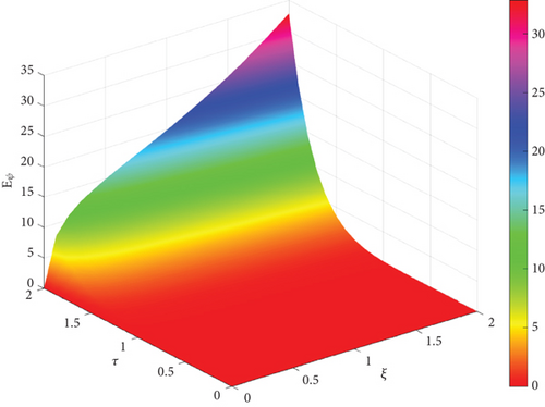
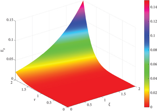
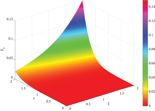
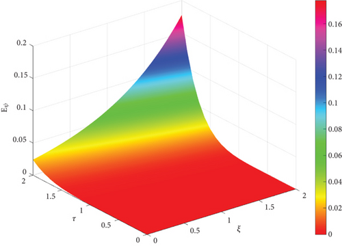
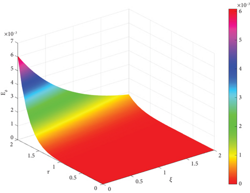
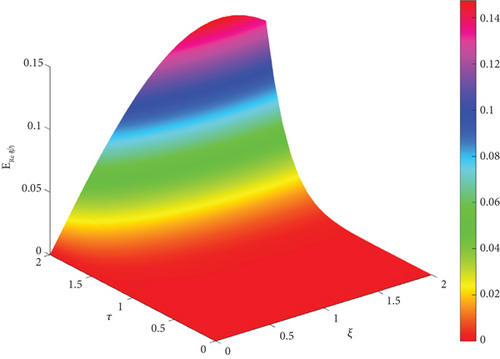
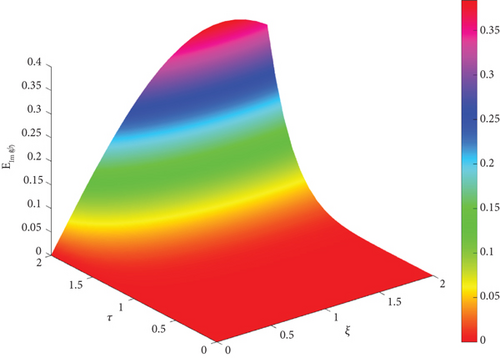
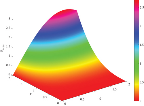
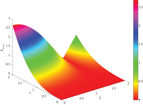
The primary aim of this section is to demonstrate the application of MRDTM through the following examples, demonstrating the method’s accuracy and effectiveness. Numerical results for Examples 1–7 are displayed in Tables 2, 3, 4, 5, 6, 7, and 8 and Figures 1, 2, 3, 4, 5, 6, 7, 8, 9, 10, 11, and 12. Within these tables, the terms ψ_E, , and E_ψ denote the exact solution, the sixth-order approximate solution of RDTM, and the absolute error of ψ, respectively.

Example 1. Consider the nonlinear Klein–Gordon equation:

()

Table 2. Numerical results of Example 1.

τ = ξ		ψ_E	E_ψ
0	0	0	0
0.2	0.1960133156	0.1960133156	1.27 × 10⁻¹¹
0.4	0.3684243911	0.3684243976	6.49 × 10⁻⁹
0.6	0.4952011200	0.4952013689	2.49 × 10⁻⁷
0.8	0.5573620622	0.5573653675	3.31 × 10⁻⁶
1	0.5402777778	0.5403023059	2.45 × 10⁻⁵

Table 3. Numerical results of Example 2.

τ = ξ		ψ_E	E_ψ
0	0	0	0
0.2	1.3108321938	2.6216649889	6.01 × 10⁻⁷
0.4	2.5276057834	5.0553164486	1.05 × 10⁻⁴
0.6	4.3676026484	8.7373993667	2.19 × 10⁻³
0.8	7.3112965335	14.6421514858	1.96 × 10⁻²
1	12.0863354267	24.2827641839	1.10 × 10⁻¹

Table 4. Numerical results of Example 3.

τ = ξ	Numerical results ofψ
τ = ξ		ψ_E	E_ψ
0	2	2	0
0.2	2.4918246945	2.4918246976	3.18 × 10⁻⁹
0.4	3.2255404182	3.2255409285	5.10 × 10⁻⁷
0.6	4.3201059893	4.3201169227	1.09 × 10⁻⁵
0.8	5.9529296646	5.9530324244	1.03 × 10⁻⁴
1	8.3884410254	8.3890560989	6.15 × 10⁻⁴
τ = ξ	Numerical results ofϕ
τ = ξ		ϕ_E	E_ϕ
0	0	0	0
0.2	0.0000000030	0	3.03 × 10⁻⁹
0.4	0.0000004617	0	4.62 × 10⁻⁷
0.6	0.0000094093	0	9.41 × 10⁻⁶
0.8	0.0000841064	0	8.41 × 10⁻⁵
1	0.0004787285	0	4.79 × 10⁻⁴

Table 5. Numerical results of Example 4.

τ = ξ	Numerical results ofψ
τ = ξ		ψ_E	E_ψ
0	1	1	0
0.2	1.4918246945	1.4918246976	3.18 × 10⁻⁹
0.4	2.2255404182	2.2255409285	5.10 × 10⁻⁷
0.6	3.3201059893	3.3201169227	1.09 × 10⁻⁵
0.8	4.9529296646	4.9530324244	1.03 × 10⁻⁴
1	7.3884410254	7.3890560989	6.15 × 10⁻⁴
τ = ξ	Numerical results ofϕ
τ = ξ		ϕ_E	E_ϕ
0	1	1	0
0.2	1.0000000030	1	3.03 × 10⁻⁹
0.4	1.0000004617	1	4.62 × 10⁻⁷
0.6	1.0000094093	1	9.41 × 10⁻⁶
0.8	1.0000841064	1	8.41 × 10⁻⁵
1	1.0004787285	1	4.79 × 10⁻⁴

Table 6. Numerical results of Example 5.

τ = ξ	Numerical results ofψ
τ = ξ		ψ_E	E_ψ
0	0	0	0
0.2	0.2426552717	0.2426552686	3.10 × 10⁻⁹
0.4	0.5809443847	0.5809439008	4.84 × 10⁻⁷
0.6	1.0288557364	1.0288456663	1.01 × 10⁻⁵
0.8	1.5965971273	1.5965053406	9.18 × 10⁻⁵
1	2.2878872056	2.2873552872	5.32 × 10⁻⁴
τ = ξ	Numerical results ofϕ
τ = ξ		ϕ_E	E_ϕ
0	1	1	0
0.2	0.8024106473	0.8024106473	5.20 × 10⁻¹¹
0.4	0.6174056370	0.6174056479	1.09 × 10⁻⁸
0.6	0.4529535614	0.4529537891	2.28 × 10⁻⁷
0.8	0.3130486476	0.3130505040	1.86 × 10⁻⁶
1	0.1987570870	0.1987661103	9.02 × 10⁻⁶

Table 7. Numerical results of Example 6.

τ = ξ		ψ_E	E_ψ
τ = ξ		ψ_E	E_Re(ψ)	E_Im(ψ)
0	0	0	0	0
0.2	0.1897960607 − 0.0587108103i	0.1897960610 − 0.0587108017i	3.2 × 10⁻¹⁰	8.6 × 10⁻⁹
0.4	0.3214006654 − 0.2198842881i	0.3214008270 − 0.2198821360i	1.62 × 10⁻⁷	2.15 × 10⁻⁶
0.6	0.3509814156 − 0.4423526300i	0.3509873900 − 0.4422996437i	5.97 × 10⁻⁶	5.3 × 10⁻⁵
0.8	0.2598642525 − 0.6691038508i	0.2599395423 − 0.6686039153i	7.53 × 10⁻⁵	5.0 × 10⁻⁴
0	0.0590015788 − 0.8421283840i	0.0595233027 − 0.8393630887i	5.22 × 10⁻⁴	2.77 × 10⁻³

Table 8. Numerical result of Example 7.

τ = ξ		ω_E	E_ω
τ = ξ		ω_E	E_Re(ω)	E_Im(ω)
0	1	1	0	0
0.2	0.9205312086 + 0.3920318557i	0.9210609940 + 0.3894183423i	5.30 × 10⁻⁴	2.60 × 10⁻³
0.4	0.6883989768 + 0.7370056845i	0.6967067093 + 0.7173560909i	8.31 × 10⁻³	1.96 × 10⁻²
0.6	0.3217000334 + 0.9914675773i	0.3623577545 + 0.9320390860i	4.07 × 10⁻²	5.94 × 10⁻²
0.8	−0.1516607592 + 1.1185039848i	−0.0291995223 + 0.9995736030i	1.22 × 10⁻¹	1.19 × 10⁻¹
	−0.6968150780 + 1.0894832831i	−0.4161468365 + 0.9092974268i	2.81 × 10⁻¹	1.80 × 10⁻¹

Details are in the caption following the image — **Figure 1**
Open in figure viewer PowerPoint

3D plot of the surface of E_ψ in Example 1.

Applying the RDT to Equation (15) yields the recurrent relation:

()

and from the initial conditions in (15), we have

()

Substituting in Equation (16), we obtain

()

The sixth-order RDTM series solution of Equation (15) is attained via the inverse transformation in Equation (2) as

()

The Laplace transform with respect to τ for Equation (19) yields

()

Letting s = 1/τ, we have

()

The Padé approximants give

()

where [3/3](τ) represents a Padé approximant of order [3/3], meaning both the numerator and denominator are polynomials of degree at most three.

Recalling τ = 1/s, we obtain

()

Finally, applying the inverse Laplace transform ℓ⁻¹ to Equation (33), we obtain

()

which is the exact solution of Equation (25).

Example 2. Consider the nonlinear reaction-diffusion-convection equation:

()

Applying the RDT to Equation (25) yields the recurrent relation:

()

and from the initial conditions in (25), we have

()

Substituting in Equation (26), we obtain

()

The sixth-order RDTM series solution of Equation (25) is attained via the inverse transformation in Equation (2) as

()

The Laplace transform with respect to τ for Equation (29) yields

()

Letting s = 1/τ, we have

()

The Padé approximants give

()

Recalling τ = 1/s, we obtain

()

Finally, applying ℓ⁻¹ to Equation (23), we obtain

which is the exact solution of Equation (15).

Example 3. Consider the following system of linear PDEs:

()

Applying the RDT to Equation (34) yields the recurrent relation:

()

and from the initial conditions in (34), we have

()

Substituting in Equation (35), we obtain

()

The sixth-order RDTM series solution of Equation (34) is attained via the inverse transformation in Equation (2) as

()

The Laplace transform with respect to τ for Equation (38) yields

()

Letting s = 1/τ, we have

()

The Padé approximants give

()

Recalling τ = 1/s, we obtain

()

Finally, applying ℓ⁻¹ to Equation (42), we obtain

()

which is the exact solution of Equation (34).

Example 4. Consider the following system of nonlinear PDEs:

()

Following the same approach as in previous examples, the sixth-order RDTM series solution of Equation (44) is

()

The Laplace transform with respect to τ for Equation (45) yields

()

where the substitution s = 1/τ is applied. By applying Padé approximants and recalling τ = 1/s, we get

()

Finally, applying ℓ⁻¹ to Equation (47), we obtain the exact solution of Equation (44):

()

Example 5. Consider a system characterized by two nonlinear equations:

()

The sixth-order RDTM series solution of Equation (49) is

()

The Laplace transform with respect to τ for Equation (50) yields:

()

where the substitution s = 1/τ is applied. By applying Padé approximants and recalling τ = 1/s, we get

()

Finally, applying ℓ⁻¹ to Equation (52), we obtain the exact solution of Equation (49):

()

Example 6. Consider the following Schrödinger equation:

()

Applying the RDT to Equation (54) yields the recurrent relation:

()

where

and

are the conjugate of ψ. From the initial conditions in Equation (54), we have

()

Substituting in Equation (55), we obtain

()

The sixth-order RDTM series solution of Equation (54) is attained via the inverse transformation in Equation (2) as

()

The Laplace transform with respect to τ for Equation (58) yields

()

Letting s = 1/τ, we have

()

The Padé approximants give

()

Recalling τ = 1/s, we obtain

()

Finally, applying ℓ⁻¹ to Equation (62), we obtain

()

which is the exact solution of Equation (54).

Example 7. Consider the following system:

()

Let us define ω = ψ + iϕ, where i² = −1. The system can be expressed as

()

The sixth-order RDTM series solution of Equation (65) is

()

The Laplace transform with respect to τ for Equation (66) yields

()

where the substitution s = 1/τ is applied. By applying Padé approximants and recalling τ = 1/s, we get

()

Finally, applying ℓ⁻¹ to Equation (68), we obtain the exact solution of Equation (65):

()

5. Results and Discussion

To provide a thorough evaluation of MRDTM, we present numerical and graphical analyses highlighting its accuracy, stability, and convergence behavior compared to RDTM. One key observation is that MRDTM yields analytical solutions, regardless of the complexity of the governing equation. This characteristic is particularly valuable in applications such as engineering and physics, where even minor numerical discrepancies can lead to significant errors in practical computations. Furthermore, a closer examination of the graphical trends reveals that MRDTM converges at a near-instantaneous rate for smooth PDEs while maintaining its efficiency even in cases where nonlinearities are dominant.

Error propagation is a common issue in numerical analysis, especially with nonlinear or coupled PDEs. Traditional methods, such as finite difference and spectral approaches, often require stability constraints or corrective steps to prevent error buildup. MRDTM eliminates these concerns by using Laplace transforms and Padé approximants to construct solutions directly. Tables 2, 3, 4, 5, 6, 7, and 8 in this study show that absolute errors remain within computational precision, effectively mitigating truncation-induced inaccuracies. Furthermore, error plots confirm MRDTM’s stability across various problem structures, even for PDEs with strong nonlinearities or complex boundary conditions. Unlike finite difference and spectral methods, MRDTM does not accumulate residual errors over iterations, making it particularly effective in high-precision computational modeling, such as quantum mechanics simulations, where numerical instability can significantly affect results.

As ξ and τ move further from 0, RDTM’s accuracy decreases, as seen in the growing absolute error (E_ψ). This highlights RDTM’s limitation in maintaining precision over a broader variable range. In contrast, MRDTM consistently produces exact solutions across all tested values, demonstrating its resilience in solving complex systems without accuracy loss. The figures illustrate this clearly, showing RDTM’s increasing absolute error as ξ and τ grow, reinforcing MRDTM’s reliability. The numerical tables further highlight its advantage, comparing MRDTM’s exact solutions with RDTM’s truncated series approximations. The results emphasize MRDTM’s superior precision, particularly in cases where traditional methods struggle to sustain accuracy.

Examining the method’s convergence behavior highlights another key strength. Unlike iterative techniques, where convergence refers to an approximation progressively approaching the true solution, MRDTM provides a direct formulation that avoids successive refinements. The main question is how efficiently it performs across different PDE types. Our results show that it converges rapidly with significantly fewer terms than conventional series-based methods. This advantage is particularly evident in problems with higher-order nonlinearities, where standard approaches require extensive terms to achieve reasonable accuracy. The combination of Laplace transforms and Padé approximants accelerates the process, making it highly effective in applications such as aerodynamics, wave propagation, and material science. Furthermore, for equations with steep gradients or discontinuities, where spectral methods often struggle with Gibbs phenomena, it maintains accuracy without introducing oscillatory artifacts. A comparative study with alternative solvers could further highlight its advantages in handling problems with varying smoothness properties.

Beyond numerical validation, the practical significance of MRDTM cannot be overlooked. The equations examined in this study, including the Klein–Gordon equation, the Schrödinger equation, and reaction–diffusion models, are fundamental in many scientific and engineering applications. Obtaining exact solutions for these equations without numerical artifacts or instability is a major advantage in fields such as semiconductor physics, structural analysis, and computational fluid dynamics (CFD). Furthermore, MRDTM’s ability to handle both real and complex-valued problems extends its applicability beyond theoretical research. In engineering simulations, where PDEs govern material behavior, thermal systems, and electromagnetic waves, having an exact analytical solution minimizes the need for extensive parameter tuning and iterative corrections, making MRDTM a compelling alternative to traditional numerical solvers. One example of this advantage is in CFD, where high-precision solutions for the Navier–Stokes equations are essential for aerodynamic simulations. The efficiency of MRDTM in handling complex nonlinear PDEs suggests its potential as a valuable tool in CFD applications, reducing computational costs while ensuring accuracy in turbulence modeling.

Future work could explore its integration with hybrid analytical–numerical techniques or machine learning models to extend its applicability even further. However, as it stands, MRDTM offers a stable, efficient, and highly accurate framework for solving PDEs in physics, engineering, and applied mathematics. While MRDTM proves to be highly effective in this study, certain limitations remain. The current analysis has primarily addressed a specific class of PDEs with relatively straightforward boundary conditions. Extending this approach to more intricate boundary constraints or higher-dimensional models may necessitate further adaptations to preserve its computational efficiency and accuracy. Moreover, although the method demonstrates strong performance across the selected test cases, its effectiveness in handling highly stiff systems warrants additional investigation. Overcoming these challenges opens avenues for future research to broaden the method’s applicability to a wider spectrum of complex problems.

6. Conclusion

This research highlights the potency of MRDTM as a robust and effective tool for solving a wide range of PDEs. These classes of PDEs encompass nonlinear PDEs with real and complex variables, as well as systems of linear and nonlinear PDEs. Our findings indicate that the integration of this technique successfully enables MRDTM to find exact solutions for the considered PDEs. We begin the procedure by obtaining a series solution for the PDE via RDTM. Next, we utilize Laplace transform to RDTM truncated series solution to expand the convergence domain, enhancing the method’s effectiveness. Padé approximants are used to truncate series and acquire a meromorphic function, thus significantly contributing to the attainment of exact solutions. Finally, the required solution is attained by the inverse Laplace transform.

The efficiency of the method is demonstrated by successfully finding the exact solutions. The proposed examples demonstrate that the method greatly enhances the convergence rate, expands the convergence domain, and leads to exact solutions. MRDTM can handle diverse classes of PDEs, underscoring its potential utility in mathematics and engineering, where exact solutions are often sought but elusive.

Conflicts of Interest

The authors declare no conflicts of interest.

Funding

This research did not receive any specific external funding.

Open Research

Data Availability Statement

No underlying data was collected or produced in this study.

References

1 He J.-H., Homotopy Perturbation Technique, Computer Methods in Applied Mechanics and Engineering. (1999) 178, no. 3-4, 257–262, https://doi.org/10.1016/S0045-7825(99)00018-3, 2-s2.0-0032672778.
10.1016/S0045-7825(99)00018-3
Web of Science® Google Scholar
2 Alkhazaleh O., Modification of Homotopy Perturbation Method for Addressing Systems of PDEs, Partial Differential Equations in Applied Mathematics. (2025) 101065, https://doi.org/10.1016/j.padiff.2024.101065.
10.1016/j.padiff.2024.101065
Google Scholar
3 Jameel A., Shather A., Anakira N., Alomari A., and Saaban A., Comparison for the Approximate Solution of the Second-Order Fuzzy Nonlinear Differential Equation With Fuzzy Initial Conditions, Mathematics and Statistics. (2020) 8, no. 5, 527–534, https://doi.org/10.13189/ms.2020.080505.
10.13189/ms.2020.080505
Google Scholar
4 Vazquez-Leal H., Khan Y., Fernandez-Anaya G., Herrera-May A., Sarmiento-Reyes A., Filobello-Nino U., Jimenez-Fernandez V. M., and Pereyra-Diaz D., A General Solution for Troesch’s Problem, Mathematical Problems in Engineering. (2012) 2012, no. 1, 208375, https://doi.org/10.1155/2012/208375, 2-s2.0-84871825047.
10.1155/2012/208375
Google Scholar
5 Guerrero F., Santonja F. J., and Villanueva R. J., Solving a Model for the Evolution of Smoking Habit in Spain With Homotopy Analysis Method, Nonlinear Analysis: Real World Applications. (2013) 14, no. 1, 549–558, https://doi.org/10.1016/j.nonrwa.2012.07.015, 2-s2.0-84866403094.
10.1016/j.nonrwa.2012.07.015
Web of Science® Google Scholar
6 Anakira N. R., Alomari A. K., and Hashim I., Application of Optimal Homotopy Asymptotic Method for Solving Linear Delay Differential Equations, AIP Conference Proceedings, 2013, 1571, no. 1, American Institute of Physics, 1013–1019.
Google Scholar
7 Vazquez-Leal H., Generalized Homotopy Method for Solving Nonlinear Differential Equations, Computational and Applied Mathematics. (2014) 33, no. 1, 275–288, https://doi.org/10.1007/s40314-013-0060-4, 2-s2.0-84898760325.
10.1007/s40314-013-0060-4
Web of Science® Google Scholar
8 Khan Y., Vazquez-Leal H., Hernandez-Martinez L., and Faraz N., Variational Iteration Algorithm-II for Solving Linear and Non-Linear ODEs, International Journal of the Physical Sciences. (2012) 7, no. 25, 3099–4002.
10.5897/IJPS12.258
Google Scholar
9 Sadeghi Goghary H., Javadi S., and Babolian E., Restarted Adomian Method for System of Nonlinear Volterra Integral Equations, Applied Mathematics and Computation. (2005) 161, no. 3, 745–751, https://doi.org/10.1016/j.amc.2003.12.072, 2-s2.0-10644283777.
10.1016/j.amc.2003.12.072
Web of Science® Google Scholar
10 Biazar J., Babolian E., and Islam R. M., Solution of a System of Volterra Integral Equations of the First Kind by Adomian Method, Applied Mathematics and Computation. (2003) 139, no. 2-3, 249–258, https://doi.org/10.1016/S0096-3003(02)00173-X, 2-s2.0-0037448167.
10.1016/S0096-3003(02)00173-X
Web of Science® Google Scholar
11 Ayaz F., Solutions of the System of Differential Equations by Differential Transform Method, Applied Mathematics and Computation. (2004) 147, no. 2, 547–567, https://doi.org/10.1016/S0096-3003(02)00794-4, 2-s2.0-0141961581.
10.1016/S0096-3003(02)00794-4
Web of Science® Google Scholar
12 Arifeen S. U., Haq S., Ali I., and Aldosary S. F., Galerkin Approximation for Multi-Term Time-Fractional Differential Equations, Ain Shams Engineering Journal. (2024) 15, no. 7, 102806, https://doi.org/10.1016/j.asej.2024.102806.
10.1016/j.asej.2024.102806
Google Scholar
13 Arifeen S. U. and Haq S., Petrov–Galerkin Approximation of Time-Fractional Coupled Korteweg–de Vries Equation for Propagation of Long Wave in Shallow Water, Mathematics and Computers in Simulation. (2023) 207, 226–242, https://doi.org/10.1016/j.matcom.2022.12.028.
10.1016/j.matcom.2022.12.028
Google Scholar
14 Ala’yed O., Saadeh R., and Qazza A., Numerical Solution for the System of Lane-Emden Type Equations Using Cubic B-Spline Method Arising in Engineering, AIMS Mathematics. (2023) 8, no. 6, 14747–14766, https://doi.org/10.3934/math.2023754.
10.3934/math.2023754
Google Scholar
15 Ala′yed O., Ying T. Y., and Saaban A., Numerical Solution of First Order Initial Value Problem Using Quartic Spline Method, AIP Conference Proceedings 1691, 2015, AIP Publishing, https://doi.org/10.1063/1.4937053, 2-s2.0-84984548934.
10.1063/1.4937053
Google Scholar
16 AlA′Yed O., Ying T. Y., and Saaban A., Quintic Spline Method for Solving Linear and Nonlinear Boundary Value Problems, Sains Malaysiana. (2016) 45, 1007–1012.
Google Scholar
17 Ala′yed O., Batiha B., Abdelrahim R., and Jawarneh A., On the Numerical Solution of the Nonlinear Bratu Type Equation Via Quintic B-Spline Method, Journal of Interdisciplinary Mathematics. (2019) 22, no. 4, 405–413, https://doi.org/10.1080/09720502.2019.1624305, 2-s2.0-85068158126.
10.1080/09720502.2019.1624305
Google Scholar
18 Ala’yed O., Qazza A., Saadeh R., and Alkhazaleh O., A Quintic B-Spline Technique for a System of Lane-Emden Equations Arising in Theoretical Physical Applications, AIMS Mathematics. (2024) 9, no. 2, 4665–4683, https://doi.org/10.3934/math.2024225.
10.3934/math.2024225
Google Scholar
19 Batiha B., Ghanim F., Alayed O., Hatamleh R. E., Heilat A. S., Zureigat H., and Bazighifan O., Solving Multispecies Lotka–Volterra Equations by the Daftardar-Gejji and Jafari Method, International Journal of Mathematics and Mathematical Sciences. (2022) 2022, 7, https://doi.org/10.1155/2022/1839796, 1839796.
10.1155/2022/1839796
Google Scholar
20 Zhu J. Z., The Finite Element Method: Its Basis and Fundamentals, 2013, Elsevier.
Google Scholar
21 Haq S., Arifeen S. U., and Noreen A., An Efficient Computational Technique for Higher-Order KdV Equation Arising in Shallow Water Waves, Applied Numerical Mathematics. (2023) 189, 53–65, https://doi.org/10.1016/j.apnum.2023.03.012.
10.1016/j.apnum.2023.03.012
Google Scholar
22 Strang G. and Fix G. J., An Analysis of the Finite Element Method, 1973, Prentice-Hall.
Google Scholar
23 Abdelrahim R., Omar Z., Ala’yed O., and Batiha B., Hybrid Third Derivative Block Method for the Solution of General Second Order Initial Value Problems With Generalized One Step Point, European Journal of Pure and Applied Mathematics. (2019) 12, no. 3, 1199–1214, https://doi.org/10.29020/nybg.ejpam.v12i3.3425.
10.29020/nybg.ejpam.v12i3.3425
Google Scholar
24 Keskin Y. and Oturanc G., Reduced Differential Transform Method for Partial Differential Equations, International Journal of Nonlinear Sciences and Numerical Simulation. (2009) 10, no. 6, 741–749, https://doi.org/10.1515/IJNSNS.2009.10.6.741, 2-s2.0-69149087769.
10.1515/IJNSNS.2009.10.6.741
Web of Science® Google Scholar
25 Keskin Y. and Oturanc G., The Reduced Differential Transform Method: A New Approach to Fractional Partial Differential Equations, Nonlinear Science Letters A. (2010) 1, no. 2, 207–217.
Google Scholar
26 Keskin Y. and Oturanc G., Reduced Differential Transform Method for Generalized KdV Equations, Mathematical and Computational Applications. (2010) 15, no. 3, 382–393, https://doi.org/10.3390/mca15030382.
10.3390/mca15030382
Google Scholar
27 Zhou J. K., Differential Transformation and Its Applications for Electrical Circuits, [in Chinise], 1986, Huazhong University Press.
Google Scholar
28 Batiha A. M. and Batiha B., Differential Transformation Method for a Reliable Treatment of the Nonlinear Biochemical Reaction Model, Advanced studies in Biology. (2011) 3, 355–360.
Google Scholar
29 Durur H., Ilhan E., and Bulut H., Novel Complex Wave Solutions of the (2+1)-Dimensional Hyperbolic Nonlinear Schrödinger Equation, Fractal and Fractional. (2020) 4, no. 3, https://doi.org/10.3390/fractalfract4030041.
10.3390/fractalfract4030041
Web of Science® Google Scholar
30 Gao W., Veeresha P., Prakasha D. G., Senel B., and Baskonus H. M., Iterative Method Applied to the Fractional Nonlinear Systems Arising in Thermoelasticity With Mittag-Leffler Kernel, Fractals. (2020) 28, no. 8, https://doi.org/10.1142/S0218348X2040040X, 2040040.
10.1142/S0218348X2040040X
Google Scholar
31 Gao W., Senel M., Yel G., Baskonus H. M., and Senel B., New Complex Wave Patterns to the Electrical Transmission Line Model Arising in Network System, AIMS Mathematics. (2020) 5, no. 3, 1881–1892, https://doi.org/10.3934/math.2020125.
10.3934/math.2020125
Google Scholar
32 Al-Refai M., Maximum Principles for Nonlinear Fractional Differential Equations in Reliable Space, Progress in Fractional Differentiation and Applications. (2020) 6, no. 2, 95–99, https://doi.org/10.18576/pfda/060202.
10.18576/pfda/060202
Google Scholar
33 García Guirao J. L., Baskonus H. M., and Kumar A., Regarding New Wave Patterns of the Newly Extended Nonlinear (2 + 1)-Dimensional Boussinesq Equation With Fourth Order, Mathematics. (2020) 8, no. 3, https://doi.org/10.3390/math8030341.
10.3390/math8030341
Google Scholar
34 Yel G., Baskonus H. M., and Gao W., New Dark–Bright Soliton in the Shallow Water Wave Model, AIMS Mathematics. (2020) 5, no. 4, 4027–4044, https://doi.org/10.3934/math.2020259.
10.3934/math.2020259
Google Scholar
35 Momani S. M. and Erturk V. S., Solutions of Non-Linear Oscillators by the Modified Differential Transform Method, Computers & Mathematics with Applications. (2008) 55, no. 4, 833–842, https://doi.org/10.1016/j.camwa.2007.05.009, 2-s2.0-37649020448.
10.1016/j.camwa.2007.05.009
Web of Science® Google Scholar
36 Abazari R. and Ganji M., Extended Two-Dimensional DTM and Its Application on Nonlinear PDEs With Proportional Delay, International Journal of Computer Mathematics. (2011) 88, no. 8, 1749–1762, https://doi.org/10.1080/00207160.2010.526704, 2-s2.0-79956153100.
10.1080/00207160.2010.526704
Web of Science® Google Scholar
37 Jafari H., Jassim H. K., Moshokoa S. P., Ariyan V. M., and Tchier F., Reduced Differential Transform Method for Partial Differential Equations Within Local Fractional Derivative Operators, Advances in Mechanical Engineering. (2016) 8, no. 4, 1687814016633013, https://doi.org/10.1177/1687814016633013, 2-s2.0-84967110136.
10.1177/1687814016633013
Google Scholar
38 Keskin Y., Servi S., and Oturanç G., Reduced Differential Transform Method for Solving Klein Gordon Equations, Proceedings of the World Congress on Engineering, 2011, 1, WCE.
Google Scholar
39 Baker G. A., Essentials of Padé Approximants, 1975, Academic Press.
Google Scholar
40 Benhammouda B., Vazquez-Leal H., and Sarmiento-Reyes A., Modified Reduced Differential Transform Method for Partial Differential Algebraic Equations, Journal of Applied Mathematics. (2014) 2014, 9, https://doi.org/10.1155/2014/279481, 2-s2.0-84937032001, 279481.
10.1155/2014/279481
Google Scholar

All articles

A Study of Solutions for Some Classes of PDEs Arising in Physics and Engineering Using Modified Reduced Differential Transform Method

Abstract

1. Introduction

2. Preliminaries

2.1. RDT

2.2. Padé Approximation

3. Main Results

4. Implementations

5. Results and Discussion

6. Conclusion

Conflicts of Interest

Funding

Open Research

Data Availability Statement

References

Figures

References

Information

About Wiley Online Library

Help & Support

Opportunities

Connect with Wiley

A Study of Solutions for Some Classes of PDEs Arising in Physics and Engineering Using Modified Reduced Differential Transform Method

Abstract

1. Introduction

2. Preliminaries

2.1. RDT

2.2. Padé Approximation

3. Main Results

4. Implementations

5. Results and Discussion

6. Conclusion

Conflicts of Interest

Funding

Open Research

Data Availability Statement

References

Figures

References

Related

Information