International Journal of Intelligent Systems

Volume 2025, Issue 1 6833629

Research Article

Open Access

A Lightweight Dynamic Hierarchical Neural Network Model and Learning Paradigm

Liping Liao

orcid.org/0009-0004-0282-3817

School of Cyber Security , Guangdong Polytechnic Normal University , Guangzhou , China , gdin.edu.cn

Guangdong Provincial Key Laboratory of Intellectual Property and Big Data , Guangdong Polytechnic Normal University , Guangzhou , China , gdin.edu.cn

Search for more papers by this author

Junlong Lin,

Junlong Lin

School of Cyber Security , Guangdong Polytechnic Normal University , Guangzhou , China , gdin.edu.cn

Search for more papers by this author

Wenjing Zhang,

Wenjing Zhang

School of Cyber Security , Guangdong Polytechnic Normal University , Guangzhou , China , gdin.edu.cn

College of Cyber Security , Jinan University , Guangzhou , China , jnu.edu.cn

Search for more papers by this author

Jun Cai,

Corresponding Author

Jun Cai

[email protected]

orcid.org/0000-0003-3293-6658

School of Cyber Security , Guangdong Polytechnic Normal University , Guangzhou , China , gdin.edu.cn

Guangdong Provincial Key Laboratory of Intellectual Property and Big Data , Guangdong Polytechnic Normal University , Guangzhou , China , gdin.edu.cn

Search for more papers by this author

Liping Liao,

Liping Liao

orcid.org/0009-0004-0282-3817

School of Cyber Security , Guangdong Polytechnic Normal University , Guangzhou , China , gdin.edu.cn

Guangdong Provincial Key Laboratory of Intellectual Property and Big Data , Guangdong Polytechnic Normal University , Guangzhou , China , gdin.edu.cn

Search for more papers by this author

Junlong Lin,

Junlong Lin

School of Cyber Security , Guangdong Polytechnic Normal University , Guangzhou , China , gdin.edu.cn

Search for more papers by this author

Wenjing Zhang,

Wenjing Zhang

School of Cyber Security , Guangdong Polytechnic Normal University , Guangzhou , China , gdin.edu.cn

College of Cyber Security , Jinan University , Guangzhou , China , jnu.edu.cn

Search for more papers by this author

Jun Cai,

Corresponding Author

Jun Cai

[email protected]

orcid.org/0000-0003-3293-6658

School of Cyber Security , Guangdong Polytechnic Normal University , Guangzhou , China , gdin.edu.cn

Guangdong Provincial Key Laboratory of Intellectual Property and Big Data , Guangdong Polytechnic Normal University , Guangzhou , China , gdin.edu.cn

Search for more papers by this author

First published: 25 March 2025

https://doi.org/10.1155/int/6833629

Academic Editor: Riccardo Ortale

Share a link

Email
Wechat
Bluesky

Abstract

In image analysis scenarios such as the Internet of Things and the metaverse, the introduction of federated learning (FL) is an effective solution to safeguard user data security and meet low-latency requirements during the machine learning process. However, due to the constrained computational power and memory of devices, facilitating the local training of complex models becomes challenging, thereby posing a significant obstacle to the application of FL. Consequently, a lightweight dynamic hierarchical neural network model and its learning paradigm are proposed in this study. Specifically, a lightweight compression method is designed based on enlarged receptive fields and separable convolutions to reduce redundancy in convolutional layer feature maps. A dynamic model partitioning method is devised, grounded in the Q-Learning reinforcement learning algorithm, to enable collaborative model training across multiple devices and enhance the utilization efficiency of device computing and storage resources. Furthermore, a hierarchical federated partition learning (HFSL) paradigm based on complete weight sharing is introduced to facilitate the compatibility of partitioned models with FL. Experimental results show that our lightweight model outperforms existing models in terms of accuracy, lightweight degree, and efficiency on image analysis tasks. Moreover, the proposed HFSL paradigm achieves performance comparable to centralized training.

1. Introduction

In the current digital era, research on machine learning (ML) models within the context of the Internet of Things (IoT) and metaverse has increasingly become a focal point for cutting-edge technology and business innovation [1]. Using the vast amounts of data generated by devices for ML, particularly through convolutional neural networks (CNNs), can significantly enhance the automation and intelligence of systems. For instance, through the utilization of image data captured by cameras in factory settings to train CNN models, it becomes possible to offer diagnostic services for safety incidents within industrial facilities, while also facilitating high-quality image analysis for industrial metaverses. Typically, constructing high-accuracy CNN models requires collecting extensive training data. However, transmitting raw data from devices to a central node may raise concerns issues of user privacy and data security. Federated learning (FL), as an emerging distributed ML paradigm, enables model training and refinement without sharing sensitive data. Specifically, during each FL epoch, the CNN model undergoes local training on devices using their private datasets. The locally trained model parameters are aggregated by a centralized server, which updates the global model parameters through a model aggregation algorithm [2]. In contexts like the IoT and the metaverse, FL serves to tackle challenges in terms of data centralization and privacy breaches. Simultaneously, it optimizes the utilization of computational resources from edge devices, thereby mitigating communication overhead [3]. By conducting model training on devices and sharing only model parameters rather than raw data, the risk of data leakage can be effectively reduced, and response times improved. Consequently, FL has been widely adopted in the scenarios such as smart factories, virtual reality, smart homes, and smart cities.

In FL, CNN models are deployed and trained on devices, necessitating each device to possess sufficient computational and storage resources for executing the training tasks. Nevertheless, most devices commonly do not have such computational capabilities and memory for this training purpose, which brings barrier for FL to be practically applied [4]. Take VGG-16 as an example, whose parameters are up to 138 million, occupies over 552 MB of storage space, and requires 15.3 billion floating-point operations (BFLOPs) for processing a single image [5]. As neural networks scale up, both compute and storage requirements increase simultaneously, raising hurdles for devices that may find even the inference phase burdensome. Current research primarily focuses on model compression and pruning techniques, which aim to diminish parameter count and computation but often at the expense of model accuracy. Hence, the obstacle persists in designing lightweight model and distributed learning methodologies capable of adapting to the resource limitations of devices.

To address the challenges outlined above, this paper concentrates on devising lightweight CNN models and corresponding distributed learning paradigms to advance FL application in IoT and metaverse scenarios. Initially, by enhancing the computational logic of the convolutional layers in the CNN model, a minor compromise in model accuracy is incurred while maintaining the number of feature maps, leading to a notable decrease in model parameters and computational workload. This sets the stage for the preliminary lightweight implementation of the model on various devices. Subsequently, models that have undergone preliminary lightweighting allow for storage and operate on most devices, though the model training time may be extended due to the computational limitations of the devices. Although the extreme compression techniques, such as pruning, can substantially decrease model parameters and computation, they often reduce the number of feature maps, significantly impacting model accuracy [6]. Thus, we transcend the limitations of current research that stress the running of the entire model on a single device and extreme compression in detriment to accuracy and considered both computational latency and accuracy. To this end, a method for splitting the model and running it on two devices is proposed, alleviating the computational burden on individual device. Given that devices within the scope of FL applications are trustworthy and monitorable, training models across two devices is feasible. This approach lowers the overall computational latency without resorting to model compression techniques. Finally, adhering to the fundamental principles of FL and leveraging the advantages of split learning (SL), a distributed learning paradigm that fully shares device parameter data is formulated, compatible with the aforementioned methods. The overall technical framework is shown in Figure 1. The main contributions of this paper are presented as follows:

•
A model lightweighting method based on enhanced receptive fields and separable convolutions is put forward, which minimizes the number of parameters and computational volume. Concurrently, this approach captures more distant contextual information to enhance the model’s expressive capacity;
•
A model dynamic splitting mechanism grounded in the Q-Learning algorithm is introduced, utilizing the Gradient-weighted Class Activation Mapping (Grad-CAM) algorithm to identify optimal splitting points for the model and enabling the intelligent agent to dynamically determine the best split points;
•
Experimental results demonstrate that the refined model has 6.424 million (M) parameters, representing a reduction of 29.48%; the computational volume is 0.421 BFLOPs, displaying a decrease of 58.73%. Moreover, the model achieves a Top-1 accuracy of 71.0%, and a Top-5 accuracy of 90.0%, with only a 1.1% decrease, outperforming other similar models. Under the hierarchical federated SL (HFSL) paradigm with complete parameter sharing, accuracy remains comparable to the unsplit one.

Details are in the caption following the image — **Figure 1**
Open in figure viewer PowerPoint

Overall technical framework diagram. The framework consists of model lightweighting, model dynamic splitting, and hierarchical federated split learning, corresponding to the algorithm design process in Section 3. By dynamically determining the optimal splitting point, the CNN global model W is split into two partitions, W^l and W^m, referred to as the low-computational network and the medium-computational network, processed and calculated on low-computational and medium-computational devices K, respectively.

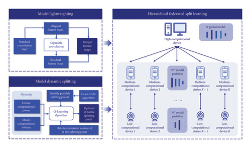
The remainder of this paper is organized in the following manner. Section 2 reviews the related work. Section 3 provides a detailed explanation of the proposed lightweight CNN model, the model’s dynamic splitting method, and the HFSL paradigm. Section 4 describes and analyzes the experimental process and results. Lastly, Section 5 brings this paper to a conclusion.

2. Related Works

2.1. Lightweight Model

Lightweight models are key for FL on devices, with techniques like compression, direct design, and neural architecture search (NAS) that reduce parameters and complexity.

In model compression, Ren et al. [7] proposed an adaptive knowledge distillation method compressing multiple teacher models into a single student model. Liu et al. [8] introduced a discrimination-aware channel pruning method which identifies key channels per layer based on discriminative loss and reconstruction, removing non-essential channels. Du, Ma, and Liu [9] presented a compression method based on knowledge distilling and adversarial learning to address model redundancy. Researchers have also explored the direct design of efficient neural networks, such as SqueezeNet [10], a CNN with an asymmetric U-shaped architecture that employs attention mechanisms to emphasize relevant features and suppress irrelevant ones through attention gates in its skip connections. ShuffleNets [11] leverage grouped convolutions and channel permutation, dividing large kernels into smaller ones for efficient computation within CNN models. MobileNets [12] are deep CNN models specifically designed for mobile devices, utilizing depthwise convolution and pointwise convolution. In NAS, Yin, Chen, and Tao [13] proposed a NAS algorithm based on policy gradient reinforcement learning and the parameter-sharing to minimize device energy consumption and model error. Shen et al. [14] presented an evolving deep multiple kernel learning network through genetic algorithm to find the best deep multiple kernel learning structure, including the weights and the topology of the model.

Model compression may impair accuracy and generalization, as reducing the model size can limit its expressiveness. The design of a tiny often leads to trade-offs in performance, making it harder to capture complex patterns. Additionally, the NAS requires substantial computational resources and time costs, making it impractical for certain applications. We propose a method enhancing high-dimensional feature maps without reducing channels, by modifying convolutional operations to lower computational load while preserving accuracy.

2.2. Model Splitting Point Selection

The selection of model splitting points is a research endeavor conducted within distributed learning scenarios to fully leverage the computational resources of different nodes, enabling the distributed processing of models and data. Shao and Zhang [15] introduced a framework with model splitting, communication-aware compression, employing exhaustive search to determine the model splitting points. Wang et al. [16] proposed a multiobjective mechanism that minimizes communication costs by transforming the multisplit issue into a minimal cost graph search and optimizing distributed algorithms. Wu et al. [17] utilized reinforcement learning and clustering to dynamically determine layer offloading for models, addressing computational heterogeneity and variable network bandwidth. Yan, Bi, and Zhang [18] investigated the joint optimization of model placement and online model splitting decisions under wireless channel fading conditions to minimize the time and communication costs for edge collaborative inference of devices. Tuli, Casale, and Jennings [19] employ decision-aware reinforcement learning to optimize between layer and semantic splitting strategies for neural network tasks on mobile edge devices, ensuring efficient and scalable computation based on service deadline requirements.

Significant research has been dedicated to refining model splitting strategies to enhance accuracy and decrease computational demands. Yet, existing methods often lack the flexibility to respond to dynamic environmental changes, leading to suboptimal performance in real-time applications. To improve performance and reduce latency, considering device and model adaptability, adaptive and dynamic model splitting strategies are essential to address fluctuating environmental conditions and ensure efficient resource utilization.

2.3. Distributed Learning Paradigm

The centralized training on large cloud servers is becoming unsustainable. To protect user privacy and ensure timely model convergence, researchers have proposed various distributed learning paradigms. For instance, FL [2] employs data from multiple clients to train neural network models, utilizing a parameter server to compute and distribute the average weights among clients. SL [20] involves the server splitting the global model parameters into multiple partitions, which are then trained sequentially with each client. After the initial client’s training is complete, its weights are shared with the next client in the training sequence. Combining FL and SL, various hybrid training methods have been introduced. Parallel SL [21] is a variant of SL where the server simultaneously trains client output on multiple batches in parallel. The client’s weight is kept confidential, while just the server’s weight is updated and transmitted. Federated reconstruction [22] parallelizes local and global weight training across clients, retaining only averaged global weights after each epoch to safeguard data privacy. Federated SL [23] combines edge servers with parallel client training, with edge weights aggregated by a parameter server and client weights kept private. Federated Edge Learning [24] is an extension of the FL paradigm, tailored to leverage the capabilities of edge computing. In a federated edge learning system, multiple edge devices collaborate to train a shared ML model while keeping the data decentralized and private.

These paradigms favor data privacy over shared client-side model weights, accepting some accuracy trade-off. However, local area networks of IoT and the metaverse, recognized as secure zones for authorized devices and users, offer a platform for extensive data sharing with controlled access. We propose a HFSL paradigm that, through complete weight sharing, diminishes the computational burden on devices, increases training data volume, and upholds both accuracy and data security, while ensuring that privacy concerns are effectively addressed.

3. Proposed Methodology

3.1. Design of Model Lightweighting

Models such as ShuffleNet [11] and MobileNet [12] have introduced depthwise convolutions or shuffle operations, employing smaller convolutional filters to construct efficient CNNs [25]. However, the remaining 1 × 1 convolutional layers still occupy a significant amount of memory and computational resources [26]. Additionally, through feature map visualization techniques, it has been observed that standard traditional convolutional operations exhibit similar feature map information, leading to computational redundancy in the model. To reduce the computation of 1 × 1 convolutions and the extensive redundancy present in feature maps within CNN models, we propose improvements to the convolutional layers of the CNN. For each convolutional layer, a small number of original feature maps are output through standard traditional convolutional operations, and the residual feature maps are generated using depthwise separable convolution operations based on the original feature maps, while retaining the identity mapping of the convolutional layer. This approach reduces the computational power required to generate partial feature maps, diminishes model feature map redundancy, and decreases the model’s computational overhead.

Let the given input feature map data be denoted as

, where H_in and W_in represent the height and width of the input feature map, and C_in is the number of input channels. The operation for generating n feature maps with a standard convolutional layer is shown in equation (1).

()

where ∗ represents the convolution operation, b is the bias term used to offset or shift the output of the convolution operation;

is the output feature map with n channels,

is the convolutional filter of the layer, C is the number of channels in the filter, and K_H × K_W is the size of the filter’s convolutional kernel. f and b are optimized parameters determined by the dimensions of the input and output feature mappings.

The output feature maps of the convolutional layer typically contain much redundancy, with some being similar to each other. There is no need to generate these redundant feature maps individually with a large amount of computational resources and parameters. Instead, m original feature maps can be generated using a standard traditional convolutional layer, as shown in equation (2).

()

where

is the output feature map with m channels, and

is the convolutional filter of the layer, with m ≤ n. The bias term b is omitted, as it does not participate in the convolution operation. The parameters such as the convolution kernel size, stride, and padding are the same as in the standard convolution operation in equation (1) to maintain consistent output feature map size.

To further obtain the required n feature maps, depthwise separable convolution is applied to each original feature map in Y^′ to generate s residual feature maps, as shown in equation (3).

()

where

is the i-th original feature map in Y^′, f_i,j is the operation using the i-th original feature map to generate the j-th remaining feature map, and the last f_i,s operation is the identity mapping for the original feature map. Through the above steps, a total of n = m + s feature maps can be obtained as the output data of the improved convolutional layer. Depthwise separable convolution operates on each channel, with a computational cost significantly lower than that of regular convolution. An example of this method is depicted in Figure 2.

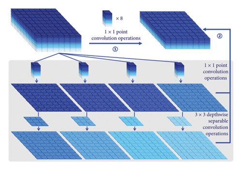
3.2. Design of Model Dynamic Splitting

To address the issue of insufficient computational capacity on individual device, it is feasible to split the model into submodels, which are then trained across different devices, thereby facilitating the training of the global model. When designing the model splitting points, it is crucial to consider the computational load and data volume of each segment, while also taking into account the dynamic changes in device computing power and their impact on model accuracy. Consequently, we have designed a model dynamic splitting mechanism based on reinforcement learning algorithms, utilizing the Q-Learning algorithm and Grad-CAM algorithm to determine the dynamic optimal splitting points for CNN models. The Grad-CAM algorithm assesses the importance of feature maps by calculating the gradients of neurons, where the gradient refers to the partial derivative of the neuron’s output with respect to the decision towards the correct category. The specific Grad-CAM algorithm is designed as follows:

Within the environment where the model resides, define all possible actions, which involve selecting different splitting points. To narrow the scope of the action space, initially employ the Grad-CAM algorithm to calculate the importance coefficients of feature maps, identifying a set of more optimal splitting points on the model, thereby preserving higher precision upon splitting at that layer. The Grad-CAM algorithm allows our method to scale and adapt to large network models. Suppose the model W has o data classification results, each composed of j(j = 1, 2, …, J) data and the model has i(i = 1, 2, …, I) layers. For each data point in every layer of each classification, use the Grad-CAM algorithm to calculate the importance coefficients of the feature maps for each layer, as shown in equation (4).

()

where

is the importance coefficient of the feature map for the j-th data in the o-th classification at the i-th layer of the model, F^i,j ∈ R^n×m×z is the feature map of the neural network at the i-th layer for the j-th data, and n, m, and z are the height, width, and number of channels of the feature map, respectively, with y^o representing the probability score of the o-th classification prediction result. Subsequently, perform a weighted sum with the selected layer’s feature map F^i,j. Finally, apply the ReLU activation function to set the negative values of the gradient to 0, obtaining the weighted activation map for the j-th data of the o-th classification at the i-th layer of the model, as shown in equation (5).

()

Thus, determine the optimal splitting point by analyzing the values of the CUmulated Importance (CUI) curve. Utilize the value of the j-th data point in the o-th classification at the i-th layer of the model, fit the values in the o-th classification data to form the curve, and then perform linear fitting on the curves of all classification images to obtain the model’s CUI_i curve. Define the local maximum values on the CUI_i curve as the possible splitting points on the model, which is the action space D_t.

With the Grad-CAM algorithm, a controlled number of action spaces can be obtained. The Q-Learning algorithm is performed to find the dynamic optimal splitting points as follows:

1.
Define the state space: Considering the changing remaining computational power of devices, the state space is defined as the S_t = (a^l, a^m, b^l, b^m) vector, where a^l represents the remaining computational power of low-computational devices, a^m represents that of medium-computational devices, b^l is the computational power size of the model’s W^l partition, and b^m is that of the model’s W^m partition. The calculation of the remaining computational power of devices is defined as a = δ × E_TOPS, where the device’s computational power is E_TOPS, and the CPU occupancy rate in the current environment of the device is δ.
2.
Define the reward function: The reward function can be defined as the reward obtained after executing a certain action in the current state. In this case, the reward function can be defined as the inference latency of the model and its compatibility with the state space. If the model requires less time to complete the inference task, a higher reward value should be given. The model’s inference time can be used as an input parameter, with the output being a reward value that is negatively correlated with the inference time. Further normalization of each influencing factor is necessary for ease of computation. The reward function is calculated as illustrated in equation (6).
()
where k₁, k₂, and k₃ are parameters used to adjust the impact of various factors on the reward, determined by the needs in different scenarios, with time being the sum of the model’s inference time and communication time, calculated as shown in equation (7).
()
where V is the transmission rate, with standard Ethernet data transfer speeds ranging from 10 Mbps to 100 Mbps, calculated in this paper using a theoretical speed of 50 Mbps, equivalent to 6.25 Mb/s. inputsize is the size of the data transmission at the model’s splitting point. Initialize the Q-value table to 0, with Q-value representing the expected return value for taking a certain action in a given state.
3.
Iterative training: At each time step, the agent selects an action from the Q-value table based on the current state and executes the action. After executing the action, the agent observes the reward signal feedback from the environment and updates the values in the Q-value table according to the feedback using the Q-Learning greedy strategy. The greedy strategy selects the action with the highest Q-value as the next action based on the current state’s Q-value table. The Q-function is described as equation (8).
()
where β is the learning rate and γ is the discount factor. This encourages the agent to selecting actions with the highest Q-value during the learning process, thereby learning the optimal splitting strategy. By dynamically determining the optimal splitting point, the CNN model W is split into two partitions, W^l and W^m, referred to as the low-computational network and the medium-computational network, processed and calculated on low-computational and medium-computational devices, respectively.

3.3. Design of the HFSL Paradigm

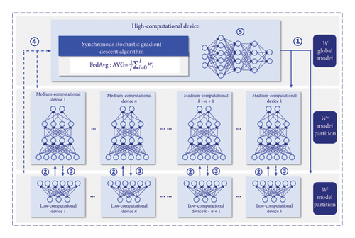
A hierarchical grouping based on the computational power of devices is proposed, categorizing them into high-computational devices capable of 10–100 BFLOPS, such as local servers and edge servers; medium-computational devices with 1–10 BFLOPS, including desktop computers, tablet computers, and gateways; and low-computational devices with 0–1 BFLOPS, such as cameras, virtual reality glasses, and smart wristbands [27]. Leveraging the respective strengths of FL and SL, while also accommodating the characteristics of the splitting model, our design facilitates the complete sharing of model weights. We have developed a HFSL paradigm based on complete weight sharing, as illustrated in Figure 3. This learning paradigm consists of one high-computational device, K medium-computational devices, and K low-computational devices, with the specific training steps as follows:

Notations: (1) S_t is a set of K low-computational devices at t time instance; (2) A_k,t is the smashed data of low-computational device k at t; (3) Y_k and

are the true and predicted labels, respectively, of the low-computational device k; (4) ∇l_k is the gradient of the loss for the low-computational device k; (5) n and n_k are the total sample size and sample size at a low-computational device k, respectively; (6) W^l and W^m are low-computational network and medium-computational network.

1.
The W^l partition of the CNN model is sent to the low-computational devices for training, which are typically the original data collection devices. The W^m partition of the CNN model is placed on the medium-computational devices for training, while the entire CNN model is subjected to weight aggregation and inference on the high-computational devices;
2.
The neural network of the W^l partition begins forward propagation on the low-computational devices, which then sends intermediate data, known as smashed data, to their corresponding medium-computational devices for the forward propagation operation of the model W^m partition. The pseudo-code for the operations executed on the low-computational devices is provided in Algorithm 1.
(3)
Upon obtaining their output labels and calculating the loss function value, the medium-computational devices initiate backward propagation. After the gradient calculation at the splitting layer is completed on the medium-computational devices, the gradients are sent back to the low-computational devices for the backward propagation computation of the W^l partition. The pseudo-code for the operations executed on the medium-computational devices is provided in Algorithm 2.
(4)
The respective low-computational and medium-computational devices send the weight parameters computed from the two partitions to the high-computational device to execute the FedAvg algorithm, updating the global CNN model. The updated weight parameters are then sent back to the low-computational and medium-computational devices for the next round of training. The pseudo-code for the operations executed on the high-computational devices is provided in Algorithm 3.
(5)
Through multiple iterative training rounds, training is terminated once the CNN model on the high-computational device achieves the desired level of accuracy. Inference is ultimately conducted on the high-computational device, and the results are subsequently transmitted to the corresponding devices for execution.

Algorithm 1: Runs on low-computational device.

Ensure: LowUpdate :
1.
Model updates ⟵ High-computational Device ()
2.
Set A_k,t = ∅
3.
for each local epoch e from 1 to Edo
4.
Forward propagation with data X_k up to a layer L ≥ 1 in ;
5.
Continue forward propagation to the remaining layers of , and get the activations of its final layer A_k,t;
6.
Y_k is the true labels of X_k;
7.
Send A_k,t and Y_k to the medium-computational device;
8.
Wait for the completion of LowBackprop (dA_k,t);
9.
end for
Ensure: LowBackprop (dA_k,t):
10.
while local epoch e ≠ Edo
11.
dA_k,t ⟵ Medium-computational Device();
12.
Back-propagation, calculate gradients with dA_k,t;
13.
Send to the High-computational device;
14.
end while

Algorithm 2: Runs on medium-computational device.

Ensure: MediumUpdate :
1.
if time instance t = 0then
2.
Model updates ⟵ High-computational Device ();
3.
else
4.
for each low-computational device k ∈ S_t in parallel do
5.
while local epoch e ≠ Edo
6.
(A_k,t, Y_k) ⟵ LowUpdate
7.
Forward propagation with A_k,t on , compute ;
8.
Loss calculation with Y_k and ;
9.
Back-propagation calculate ;
10.
Send (i.e., gradient of the A_k,t)
11.
to medium-computational device k for LowBackprop (dA_k,t);
12.
end while
13.
end for
14.
Send to the high-computational device;
15.
end if

Algorithm 3: Runs on high-computational device.

Ensure: HighExecutes :
1.
if time instance t = 0then
2.
Initialize (low-computational network);
3.
Send to all K low-computational devices for LowUpdate ;
4.
Initialize (medium-computational network)
5.
Send to all H medium-computational devices for MediumUpdate ;
6.
else
7.
for each low-computational device k ∈ S_t in parallel do
8.
⟵ LowBackprop (dA_k,t);
9.
each medium-computational device k ∈ S_t in parallel do
10.
⟵ MediumUpdate ;
11.
end for
12.
Low-computational network updates: ;
13.
Send to all K low-computational devices for LowUpdate ;
14.
Medium-computational network updates: ;
15.
Send to all K medium-computational devices for MediumUpdate ;
16.
end if

4. Experimental Results and Analysis

4.1. Experimental Environment and Datasets

The experimental environment was configured as follows: in terms of software, the operating system was Linux and the programming language was Python 3.8.0, using PyTorch as the deep learning framework. In terms of hardware configuration, the system is equipped with a 16-core CPU, 16 GB of RAM, and a 300 GB hard drive, and the Graphics Processing Unit (GPU) is an NVIDIA GeForce RTX 2080 Ti with 11 GB of GDDR6 video memory and CUDA version 11.4.

The performance of the model on the ImageNet-1K image classification dataset (ILSVRC2012) is evaluated in this study. The ImageNet-1K dataset includes 1.28 million training images and 50,000 validation images, all sized at 224 × 224. This extensive dataset covers 1000 different classes, with each class containing a minimum of 1000 images. The images are diverse, capturing a wide range of objects from the natural world, such as animals and plants, as well as man-made objects like vehicles and household items. The dataset is used to measure the accuracy of models, with performance typically reported in terms of top-1 and top-5 accuracy, which refer to the model’s ability to select the correct class as the first or within the top five choices, respectively. Images were normalized for mean and standard deviation prior to training. Specifically, the pixel values of each channel in the images were subtracted by the mean and divided by the standard deviation to center the pixel values around 0.

Additionally, weights were initialized before model training; convolutional layers employed the Kaiming initialization method, calculating the standard deviation of weights based on the weight tensor’s shape and “fan_out” approach, initializing weights to random values following a normal distribution; batch normalization layers initialized weights to 1 and biases to 0; fully connected layers initialized weights using a normal distribution with a mean of 0 and a standard deviation of 0.01, with biases set to 0. We then utilized the stochastic gradient descent optimizer to update model parameters, setting the lr learning rate parameter to 0.01, the momentum parameter to 0.9, and the weight_decay parameter to 1E − 4. The learning rate was adjusted using the cosine annealing strategy, with a batch size of 64.

4.2. Model Lightweighting Experiment

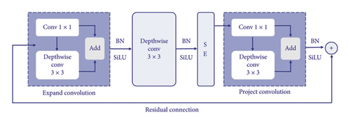
The advanced MobileNet block structure, renowned for its efficiency and widespread application, was chosen to reduce model redundancy, becoming the foundation of choice for many lightweight deep learning models. The improved lightweight block structure, denoted as MBConv-s, is illustrated in Figure 4, with the enhancements marked within the dashed. Concurrently, as the EfficientNet model is derived from NAS methods, it incorporates optimized channel and layer counts [28]. Leveraging the optimal channel and layer configurations from the EfficientNet model, we applied the MBConv-s block structure to the EfficientNet-B2 model, resulting in our refined lightweight model structure, termed EfficientNet-B2s. The EfficientNet-B2s model comprises a stem_conv, 23 MBConv-s block, a top layer, and an avgpool, as detailed in Table 1.

Table 1. Structure of the EfficientNet-B2s model.

Stage	Operator	Resolution	Channels	Layers
stem_conv	Conv3 × 3	224 × 224	32	1
1	MBConv-s, k3 × 3	112 × 112	16	a, b
2	MBConv-s, k3 × 3	112 × 112	24	a, b, c
3	MBConv-s, k5 × 5	56 × 56	48	a, b, c
4	MBConv-s, k3 × 3	28 × 28	88	a, b, c, d
5	MBConv-s, k5 × 5	14 × 14	120	a, b, c, d
6	MBConv-s, k5 × 5	14 × 14	208	a, b, c, d, e
7	MBConv-s, k3 × 3	7 × 7	352	a, b
Top	Conv1 × 1	7 × 7	1408	1
Avgpool	AdaptiveAvgPool	7 × 7	1408	1

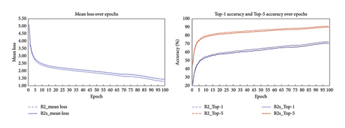
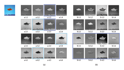
The training process before and after the model lightweight improvement is shown in Figure 5, and the comparison is shown in Table 2. It can be observed that the model’s accuracy and loss both converge better. The results indicate that our method of reducing model redundancy achieved significant improvements over the baseline model, with the model parameter count decreasing from 9.110 M to 6.424 M, a reduction of 29.48%; the model computational volume decreased from 1.020 BFLOPs to 0.421 BFLOPs, a reduction of 58.73%; meanwhile, the model storage space decreased by 28.87%, and the overall computational cache decreased by 29.08%. The model’s Top-1 accuracy is 71.0%, with only a 1.8% decrease, and the Top-5 accuracy is 90.0%, with only a 1.1% decrease. Our method significantly reduces model redundancy and computational costs while minimizing the loss of model accuracy, enhancing computational efficiency and achieving model lightweighting by replacing a large number of 1 × 1 point convolutions in the EfficientNet-B2 model with 3 × 3 depthwise separable convolutions, extracting feature maps with different receptive fields. We utilized visualization techniques to obtain feature maps generated by the convolutional layers, revealing that the EfficientNet-B2 model contained some similar feature maps with redundant information, as indicated by the same-colored frames in Figure 6(a). In contrast, the EfficientNet-B2s model reduced redundant feature maps and increased feature maps with higher-dimensional information, as boxed in Figure 6(b). Our method greatly reduces the redundancy and computational costs of the model, improving computational efficiency and achieving model lightweighting.

Table 2. Comparison before and after model lightweighting.

Model	Params (M)	FLOPs (B)	Model size (MB)	Total memory (MB)	Top-1 Acc (%)	Top-5 Acc (%)
EfficientNet-B2	9.110	1.020	37.019	163.530	72.8	91.1
EfficientNet-B2s	6.424	0.421	26.331	115.970	71.0	90.0
Improve	−29.48%	−58.73%	−28.87%	−29.08%	−1.8	−1.1

Representative models were selected for comparison, encompassing traditional convolutional, transformer-enhanced, and NAS-derived models. The comparison is presented in Table 3. The comparison shows that the computational volume of the EfficientNet-B2s model is only 35.0% of the most accurate DeiT-T model but with an accuracy difference of only 1.2%. Compared to GoogLeNet v1, SqueezeNet, ResNet-18, MobileNet v1, ShiftNet-A, MobileViTV2-0.5, and PVTv2-B0, the EfficientNet-B2s model offers higher accuracy and less computational volume. Additionally, it is observed that the EfficientNet-B2s model has a larger number of parameters than other models, which enhances the model’s performance across various tasks, including accuracy and generalization capabilities. Whether comparing model accuracy at equivalent computational volumes or comparing computational volumes at similar accuracies, our improved EfficientNet-B2s model possesses superior lightweighting advantages, making it more suitable for deployment and application in resource-constrained environments.

Table 3. Compares with other models.

Model	Params (M)	FLOPs (B)	Top-1 Acc (%)	Top-5 Acc (%)
VGG-16 [5]	138.000	15.300	71.3	90.0
GoogLeNet v1 [29]	6.798	1.550	69.8	90.9
SqueezeNet [10]	1.250	0.720	60.4	82.5
ResNet-18 [30]	11.700	1.800	70.6	—
MobileNet v1 [12]	4.250	0.569	70.6	89.5
ShiftNet-A [31]	4.100	1.400	70.1	89.7
Taylor-FO-BN [32]	7.900	1.300	71.7	—
RigL [33]	1.280	0.320	67.5	—
HRank [34]	13.800	1.600	72.0	91.0
T2T-ViT-7 [35]	4.300	1.100	71.7	—
DeiT-T [36]	5.700	1.200	72.2	—
MobileViTV2-0.5 [37]	1.400	0.466	70.2	—
PVTv2-B0 [38]	3.400	0.600	70.5	—
WD-pruning [39]	3.500	0.700	70.3	89.8
DeiT-T-X-pruner [40]	—	0.600	71.1	90.1
FLatten-PVTv2-B0 [41]	3.600	0.600	71.1	—
MGPF-VGG-16 [42]	8.280	5.500	71.0	—
DeiT-P6 [43]	3.800	0.900	70.3	—
EfficientNet-B2s (ours)	6.424	0.421	71.0	90.0

4.3. Experiment on Model Dynamic Splitting

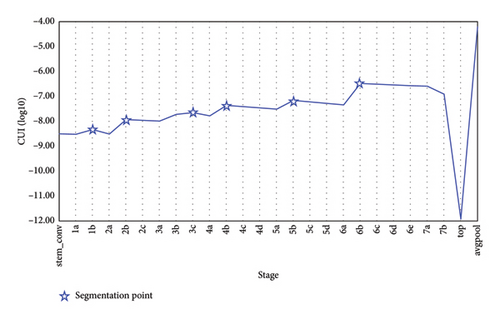
Firstly, the scope of the action space is ascertained initially through preliminary selections of splitting points. The model is structured around components such as stem, block, top, and avgpool. Considering that the convolutional backbone of the model is designed with blocks as the fundamental unit, splits are made at the block level to preserve the integrity of the basic block structure, while the final classifier, being the output layer, is not considered for splitting. We then utilize the gradient parameters saved during the training process of the EfficientNet-B2s model and employ the Grad-CAM algorithm to calculate the CUI values. These values are visualized using a line chart, with star markers indicating local maxima in the CUI curve, as depicted in Figure 7. By analyzing the CUI importance curves, we identify optimal candidate splitting points as 1b, 2b, 3c, 4b, 5b, and 6b; if the splitting point is 1b, the model is split after the 1b-block. The CUI values serve to measure the importance of each block in the model’s prediction of the correct category. Blocks with high CUI values indicate a pivotal role in making correct predictions, containing significant information related to the correct category. Therefore, when selecting the best splitting point, priority is given to preserving these key pieces of information to ensure that the model maintains high accuracy post-split.

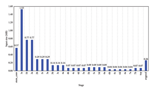
Secondly, reinforcement learning training is conducted using the state space parameter data derived from a simulated environment. The selection of splitting points is determined by the computational resource constraints of devices. The remaining computational power values of low-computational and medium-computational devices are simulated using an exponential distribution. The remaining computational power values of low-computational devices are constrained within the range of 0-1, while those of medium-computational devices are constrained within the range of 0–10, effectively mirroring the computational capabilities of real devices. Split candidate points, such as 1b, 2b, 3c, 4b, 5b, and 6b, defined in the action space, are used to calculate the computational volume data for each segment of the post-split model. The data volume at the model splitting point is derived from the computation of CUI values, as illustrated in Figure 8. Subsequently, after establishing the state space parameters and defining the action space scope, Q-Learning reinforcement learning iterative training is initiated, and the Q-values are updated based on the designed reward function. Through continuous interaction with the environment and learning, the agent can progressively refine its strategy, making optimal decisions based on the current state space parameters.

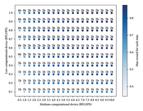
Finally, for a more effective presentation of the training results, visualization charts are utilized to illustrate the relationship between states and optimal splitting points in a more intuitive manner. The split points with the highest corresponding reward values under specific states, which are also identified as the optimal splitting points determined by the agent in that state, are selected for visualization, as depicted in Figure 9. It can be observed that when the remaining computational power value of low-computational devices exceeds that of medium-computational devices, the optimal splitting point is 6b, and the agent prefers to keep most of the model computation on the low-computational devices. When the remaining computational power value of low-computational devices is less than that of medium-computational devices, the optimal splitting points are 1b or 2b, and the agent tends to offload most of the model computation to medium-computational devices. Overall, as the remaining computational power value of the devices gradually increases, the agent tends to determine the best splitting point as 2b. This propensity stems from the medium-computational devices’ greater capability in handling more data and conducting more complex inferences; thus, making decisions at earlier splitting points can maximize rewards and minimize inference time.

4.4. HFSL Paradigm Experiment

Given that numerous articles have already validated the feasibility of end-to-end deep learning [44, 45], this paper directly proceeds to HFSL experiments to verify whether model splitting impacts the model’s accuracy. In the experiments, we selected five GeForce RTX 2080 graphics cards to conduct the experiments, simultaneously training two sets of models to simulate the training architecture of HFSL. The results of the centralized learning training, FL training, SL training, and HFSL training are shown in Figure 10.

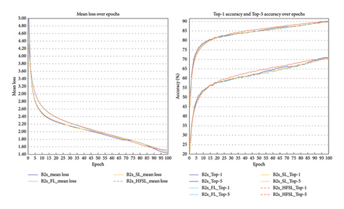
The experimental results indicate that the Top-1 accuracy is 70.7%, and the Top-5 accuracy is 89.9%. In terms of accuracy, the split model’s performance on the test set is essentially consistent with that of the unsplitting model, fluctuating within an acceptable range. This demonstrates that splitting does not significantly impair the model’s predictive capability. The complete sharing of weight parameters mitigates the loss of accuracy, as shared parameters enhance the model’s generalization and resistance to overfitting. Specifically, when weight parameters are fully shared, the sub-models resulting from the split will shar e the same parameters, implying that they influence and update each other during training. This results in a more consistent and stable feature representation learned by the global model. In terms of training speed, since the model is split into two parts and trained on different devices concurrently, the processing load is reduced, and training speed is improved. In contrast to centralized learning training, FL training, and SL training, the proposed HFSL paradigm effectively balances communication, computation, and model robustness. While FL excels at preserving privacy, it incurs higher communication costs, and SL offers advantages in reducing model size but may experience slower convergence. The HFSL paradigm, however, distributes computational tasks across multiple devices for parallel processing, improving computational resource utilization and efficiency. Additionally, since each submodel processes only partial data, the parameter updates in HFSL are more stable, which helps prevent overfitting and enhances the overall robustness of the model. This makes HFSL a more efficient and stable alternative, especially in distributed IoT and metaverse environments.

5. Conclusion

In this study, a lightweight dynamic hierarchical neural network model and its learning paradigm were proposed to advance the application of FL in IoT and metaverse scenarios. To mitigate the redundancy of convolutional layer feature maps and reduce model computational overhead, a block structure based on enhanced receptive fields and depthwise separable convolutions was designed. To tackle the computational resource constraints of devices and dynamically align device computational power with model size, a model dynamic splitting method based on the Q-Learning algorithm was introduced. To establish a distributed learning paradigm compatible with the splitting model and facilitate comprehensive sharing of device parameter data, a HFSL paradigm was proposed. Through extensive experimental validation, our lightweight model exhibited superior performance in terms of accuracy, lightweight design, and efficiency compared to existing models. Furthermore, the proposed HFSL paradigm achieved performance levels close to those of centralized training.

Looking ahead, future work will focus on proposing personalized model lightweighting solutions tailored to practical application scenarios such as anomaly detection and industrial equipment monitoring. Further efforts will be directed toward optimizing model architectures, reducing computational resource consumption, and enhancing overall system efficiency and performance. Additionally, we aim to explore the practical challenges of deploying and running such models on diverse devices, including network latency, device heterogeneity, and the dynamic adaptation of models to real-world constraints.

Conflicts of Interest

The authors declare no conflicts of interest.

Author Contributions

Liping Liao was responsible for conceptualization, methodology, and funding acquisition. Junlong Lin was the co-first author responsible for methodology, software, data curation, original draft preparation, investigation, and visualization. Wenjing Zhang was responsible for visualization and sentence optimization. Jun Cai was responsible for review and editing, validation, and funding acquisition.

Funding

This work was supported in part by the Special Projects in National Key Research and Development Program of China (2018YFB1802200, 2019YFB1804403), the Foundation of Guangdong Polytechnic Normal University (2022SDKYA029, 22GPNUZDJS26), the Key Areas of Guangdong Province (2019B010118001), the National Natural Science Foundation of China (61972104, 61902080, 62002072, 61702120), the Science and Technology Project in Guangzhou (201803010081), the Foshan Science and Technology Innovation Project, China (2018IT100283), the Guangzhou Key Laboratory (202102100006), the Science and Technology Program of Guangzhou, China (202002020035), the Industry-University-Research Innovation Fund for Chinese Universities (2021FNA04010), and the Special Project for Key Areas in General Higher Education Institutions of Guangdong Province (2023ZDZX1010).

Acknowledgments

In the preparation of this manuscript, no AI software was utilized.

Open Research

Data Availability Statement

The data that support the findings of this study are available in ImageNet at https://www.image-net.org/. These data were derived from the following resources available in the public domain:

Stanford Vision Lab, Stanford University, Princeton Universi, https://www.image-net.org/download.php.

References

1 Rajapakse V., Karunanayake I., and Ahmed N., Intelligence at the Extreme Edge: A Survey on Reformable Tinyml, ACM Computing Surveys. (2023) 55, no. 13s, 1–30, https://doi.org/10.1145/3583683.
10.1145/3583683
Web of Science® Google Scholar
2 Hu X., Cai H., Alazab M., Zhou W., Haghighi M. S., and Wen S., Federated Learning in Industrial Iot: A Privacy-Preserving Solution that Enables Sharing of Data in Hydrocarbon Explorations, IEEE Transactions on Industrial Informatics. (2024) 20, no. 3, 4337–4346, https://doi.org/10.1109/tii.2023.3306931.
10.1109/tii.2023.3306931
Web of Science® Google Scholar
3 Wang Y.-C., Xue J., Wei C., and Kuo C.-C. J., An Overview on Generative Ai at Scale With Edge-Cloud Computing, IEEE Open Journal of the Communications Society. (2023) 4, 2952–2971, https://doi.org/10.1109/ojcoms.2023.3320646.
10.1109/ojcoms.2023.3320646
Web of Science® Google Scholar
4 Lu X., Zheng H., Liu W., Jiang Y., and Wu H., Pop-fl: Towards Efficient Federated Learning on Edge Using Parallel Over-Parameterization, IEEE Transactions on Services Computing. (2024) 17, no. 2, 617–630, https://doi.org/10.1109/tsc.2024.3376194.
10.1109/tsc.2024.3376194
Web of Science® Google Scholar
5 Simonyan K. and Zisserman A., Very Deep Convolutional Networks for Large-Scale Image Recognition, 2014, https://arxiv.org/abs/1409.1556.
Google Scholar
6 Chen Z., Xiang J., Lu Y. et al., Rgp: Neural Network Pruning Through Regular Graph With Edges Swap-Ping, IEEE Transactions on Neural Networks and Learning Systems. (2024) 35, no. 10, 14671–14683, https://doi.org/10.1109/tnnls.2023.3280899.
10.1109/tnnls.2023.3280899
PubMed Google Scholar
7 Ren L., Wang T., Jia Z., Li F., and Han H., A Lightweight and Adaptive Knowledge Distillation Framework for Remaining Useful Life Prediction, IEEE Transactions on Industrial Informatics. (2023) 19, no. 8, 9060–9070, https://doi.org/10.1109/tii.2022.3224969.
10.1109/tii.2022.3224969
Web of Science® Google Scholar
8 Liu J., Zhuang B., Zhuang Z. et al., Discrimination-Aware Network Pruning for Deep Model Compression, IEEE Transactions on Pattern Analysis and Machine Intelligence. (2022) 44, no. 8, 4035–4051, https://doi.org/10.1109/TPAMI.2021.3066410.
10.1109/TPAMI.2021.3066410
PubMed Web of Science® Google Scholar
9 Du M., Ma Z., and Liu Y., Model Compression Method Based on Knowledge Distilling and Adversarial Learning, Proceedings of the Complex System Design and Management, 2023, Springer, 118–129.
Google Scholar
10 Zhang J., Zhu H., Wang P., and Ling X., Att Squeeze U-Net: A Lightweight Network for Forest Fire Detection and Recognition, IEEE Access. (2021) 9, 10 858–910 870, https://doi.org/10.1109/access.2021.3050628.
10.1109/access.2021.3050628
Web of Science® Google Scholar
11 Zhang X., Zhou X., Lin M., and Sun J., Shufflenet: An Extremely Efficient Convolutional Neural Network for Mobile Devices, Proceedings of the IEEE Conference on Computer Vision and Pattern Recognition, 2018, 6848–6856.
Google Scholar
12 Howard A. G., Zhu M., Chen B. et al., Mobilenets: Efficient Convolutional Neural Networks for Mobile Vision Applications, 2017, https://arxiv.org/abs/1704.04861.
Google Scholar
13 Yin B., Chen Z., and Tao M., Dynamic Data Collection and Neural Architecture Search for Wireless Edge Intelligence Systems, IEEE Transactions on Wireless Communications. (2023) 22, no. 1, 688–703, https://doi.org/10.1109/twc.2022.3197809.
10.1109/twc.2022.3197809
Web of Science® Google Scholar
14 Shen W., Lin W., Wu Y., Shi F., Wu W., and Li K., Evolving Deep Multiple Kernel Learning Networks Through Genetic Algorithms, IEEE Transactions on Industrial Informatics. (2023) 19, no. 2, 1569–1580, https://doi.org/10.1109/tii.2022.3206817.
10.1109/tii.2022.3206817
Web of Science® Google Scholar
15 Shao J. and Zhang J., Communication-Computation Trade-Off in Resource-Constrained Edge Inference, IEEE Communications Magazine. (2020) 58, no. 12, 20–26, https://doi.org/10.1109/mcom.001.2000373.
10.1109/mcom.001.2000373
Web of Science® Google Scholar
16 Wang S., Zhang X., Uchiyama H., and Matsuda H., Hivemind: Towards Cellular Native Machine Learning Model Splitting, IEEE Journal on Selected Areas in Communications. (2022) 40, no. 2, 626–640, https://doi.org/10.1109/jsac.2021.3118403.
10.1109/jsac.2021.3118403
Web of Science® Google Scholar
17 Wu D., Ullah R., Harvey P., Kilpatrick P., Spence I., and Varghese B., Fedadapt: Adaptive Offloading for Iot Devices in Federated Learning, IEEE Internet of Things Journal. (2022) 9, no. 21, 20 889–920 901, https://doi.org/10.1109/jiot.2022.3176469.
10.1109/jiot.2022.3176469
Web of Science® Google Scholar
18 Yan J., Bi S., and Zhang Y.-J. A., Optimal Model Placement and Online Model Splitting for Device-Edge Co-Inference, IEEE Transactions on Wireless Communications. (2022) 21, no. 10, 8354–8367, https://doi.org/10.1109/twc.2022.3165824.
10.1109/twc.2022.3165824
Web of Science® Google Scholar
19 Tuli S., Casale G., and Jennings N. R., Splitplace: Ai Augmented Splitting and Placement of Large-Scale Neural Networks in Mobile Edge Environments, IEEE Transactions on Mobile Computing. (2023) 22, no. 9, 5539–5554, https://doi.org/10.1109/tmc.2022.3177569.
10.1109/tmc.2022.3177569
Web of Science® Google Scholar
20 Gupta O. and Raskar R., Distributed Learning of Deep Neural Network Over Multiple Agents, Journal of Network and Computer Applications. (2018) 116, 1–8, https://doi.org/10.1016/j.jnca.2018.05.003, 2-s2.0-85048721526.
10.1016/j.jnca.2018.05.003
Web of Science® Google Scholar
21 Jeon J. and Kim J., Privacy-Sensitive Parallel Split Learning, Proceedings of the 2020 International Conference on Information Networking (ICOIN), 2020, IEEE, 7–9.
Google Scholar
22 Thapa C., Mahawaga Arachchige P. C., Camtepe S., and Sun L., Splitfed:When Federated Learning Meets Split Learning, Proceedings of the AAAI Conference on Artificial Intelligence. (2022) 36, no. 8, 8485–8493, https://doi.org/10.1609/aaai.v36i8.20825.
10.1609/aaai.v36i8.20825
Google Scholar
23 Zhang Z., Pinto A., Turina V., Esposito F., and Matta I., Privacy and Efficiency of Communications in Federated Split Learning, IEEE Transactions on Big Data. (2023) 9, no. 5, 1380–1391, https://doi.org/10.1109/tbdata.2023.3280405.
10.1109/tbdata.2023.3280405
Google Scholar
24 Fu S., Dong F., Shen D., Zhang J., Huang Z., and He Q., Joint Optimization of Device Selection and Resource Allocation for Multiple Federations in Federated Edge Learning, IEEE Transactions on Services Computing. (2024) 17, no. 1, 251–262, https://doi.org/10.1109/tsc.2023.3342435.
10.1109/tsc.2023.3342435
Web of Science® Google Scholar
25 Tang Y., Han K., Guo J., Xu C., Xu C., and Wang Y., Ghostnetv2: Enhance Cheap Operation With Long-Range Attention, Advances in Neural Information Processing Systems. (2022) 35, 9969–9982.
Google Scholar
26 Qin Z., Yu F., Liu C., and Chen X., How Convolutional Neural Network See the World-A Survey of Convolutional Neural Network Visualization Methods, 2018, https://arxiv.org/abs/1804.11191.
Google Scholar
27 LEA China Mobile Communications Group Terminal Co, White Paper on End-Side Computing Network, 2022, 3–6.
Google Scholar
28 Tan M. and Le Q., Efficientnet: Rethinking Model Scaling for Convolutional Neural Networks, Proceedings of the International Conference on Machine Learning, 2019, PMLR, 6105–6114.
Google Scholar
29 Szegedy C., Liu W., Jia Y. et al., Going Deeper With Convolutions, Proceedings of the IEEE Conference on Computer Vision and Pattern Recognition, 2015, 1–9, https://doi.org/10.1109/cvpr.2015.7298594, 2-s2.0-84937522268.
10.1109/cvpr.2015.7298594
Google Scholar
30 He K., Zhang X., Ren S., and Sun J., Deep Residual Learning for Image Recognition, Proceedings of the IEEE Conference on Computer Vision and Pattern Recognition, 2016, 770–778.
Google Scholar
31 Wu B., Wan A., Yue X. et al., Shift: A Zero Flop, Zero Parameter Alternative to Spatial Convolutions, Proceedings of the IEEE Conference on Computer Vision and Pattern Recognition, 2018, 9127–9135.
Google Scholar
32 Molchanov P., Mallya A., Tyree S., Frosio I., and Kautz J., Importance Estimation for Neural Network Pruning, Proceedings of the IEEE/CVF Conference on Computer Vision and Pattern Recognition, 2019, 11 264–311 272.
Google Scholar
33 Evci U., Gale T., Menick J., Castro P. S., and Elsen E., Rigging the Lottery: Making All Tickets Winners, Proceedings of the International Conference on Machine Learning, 2020, PMLR, 2943–2952.
Google Scholar
34 Lin M., Ji R., Wang Y. et al., Hrank: Filter Pruning Using High-Rank Feature Map, Proceedings of the IEEE/CVF Conference on Computer Vision and Pattern Recognition, 2020, 1529–1538.
Google Scholar
35 Yuan L., Chen Y., Wang T. et al., Tokens-to-Token Vit: Training Vision Transformers From Scratch on Imagenet, Proceedings of the IEEE/CVF International Conference on Computer Vision, 2021, 558–567.
Google Scholar
36 Touvron H., Cord M., Douze M., Massa F., Sablayrolles A., and J´egou H., Training Data-Efficient Image Transformers & Distillation Through Attention, Proceedings of the International Conference on Machine Learning, 2021, PMLR, 10 347–410 357.
Google Scholar
37 Mehta S. and Rastegari M., Separable Self-Attention for Mobile Vision Transformers, 2022, https://arxiv.org/abs/2206.02680.
Google Scholar
38 Wang W., Xie E., Li X. et al., Pvt V2: Improved Baselines With Pyramid Vision Transformer, Computational Visual Media. (2022) 8, no. 3, 415–424, https://doi.org/10.1007/s41095-022-0274-8.
10.1007/s41095-022-0274-8
CAS Web of Science® Google Scholar
39 Yu F., Huang K., Wang M., Cheng Y., Chu W., and Cui L., Width & Depth Pruning for Vision Transformers, Proceedings of the AAAI Conference on Artificial Intelligence. (2022) 36, no. 3, 3143–3151.
Google Scholar
40 Yu L. and Xiang W., X-Pruner: Explainable Pruning for Vision Transformers, Proceedings of the IEEE/CVF Conference on Computer Vision and Pattern Recognition, 2023, 24 355–424 363, https://doi.org/10.1109/cvpr52729.2023.02333.
10.1109/cvpr52729.2023.02333
Google Scholar
41 Han D., Pan X., Han Y., Song S., and Huang G., Flatten Transformer: Vision Transformer Using Focused Linear Attention, Proceedings of the IEEE/CVF International Conference on Computer Vision, 2023, 5961–5971.
Google Scholar
42 Zhang P., Tian C., Zhao L., and Duan Z., A Multi-Granularity Cnn Pruning Framework via Deformable Soft Mask With Joint Training, Neurocomputing. (2024) 572, https://doi.org/10.1016/j.neucom.2023.127189.
10.1016/j.neucom.2023.127189
Web of Science® Google Scholar
43 Liu J., Tang D., Huang Y. et al., Updp: A Unified Progressive Depth Pruner for Cnn and Vision Transformer, 2024, https://arxiv.org/abs/2401.06426.
Google Scholar
44 Bourtsoulatze E., Burth Kurka D., and Gunduz D., Deep Joint Source Channel Coding for Wireless Image Transmission, IEEE Transactions on Cognitive Communications and Networking. (2019) 5, no. 3, 567–579, https://doi.org/10.1109/tccn.2019.2919300.
10.1109/tccn.2019.2919300
Web of Science® Google Scholar
45 Lee K. and Yu N. Y., End-to-End Learning-Based Wireless Image Recognition Using the Pyramidnet in Edge Intelligence, Proceedings of the 2023 IEEE 34th Annual International Symposium on Personal, Indoor and Mobile Radio Communications (PIMRC), 2023, IEEE, 1–6.
Google Scholar

All articles

A Lightweight Dynamic Hierarchical Neural Network Model and Learning Paradigm

Abstract

1. Introduction

2. Related Works

2.1. Lightweight Model

2.2. Model Splitting Point Selection

2.3. Distributed Learning Paradigm

3. Proposed Methodology

3.1. Design of Model Lightweighting

3.2. Design of Model Dynamic Splitting

3.3. Design of the HFSL Paradigm

4. Experimental Results and Analysis

4.1. Experimental Environment and Datasets

4.2. Model Lightweighting Experiment

4.3. Experiment on Model Dynamic Splitting

4.4. HFSL Paradigm Experiment

5. Conclusion

Conflicts of Interest

Author Contributions

Funding

Acknowledgments

Open Research

Data Availability Statement

References

Figures

References

Information

About Wiley Online Library

Help & Support

Opportunities

Connect with Wiley