An Improved A ∗ Algorithm Based on Simulated Annealing and Multidistance Heuristic Function
Abstract
The traditional A ∗ algorithm has problems such as low search speed and huge expansion nodes, resulting in low algorithm efficiency. This article proposes a circular arc distance calculation method in the heuristic function, which combines the Euclidean distance and the Manhattan distance as radius, uses a deviation distance as the correction, and assignes dynamic weights to the combined distance to make the overall heuristic function cost close to reality. Furthermore, the repulsive potential field function and turning cost are introduced into the heuristic function, to consider the relative position of obstacles while minimizing turns in the path. In order to reduce the comparison of nodes with similar cost values, the bounded suboptimal method is used, and the idea of simulated annealing is introduced to overcome the local optima trapped by node expansion. Simulation experiments show that the average running time of the improved algorithm has decreased by about 70%, the number of extended nodes has decreased by 92%, and the path has also been shortened, proving the effectiveness of the algorithm improvement.
1. Introduction
The path planning of an automatic guided vehicle (AGV) refers to finding an optimal path [1] between a given starting point and an end point. At present, the commonly used path-planning algorithms are ant colony optimization (ACO) [2], A ∗ algorithm [3], rapidly exploring random trees algorithm [4], artificial potential field method [5], approximate solution [6], etc. A ∗ algorithm is widely used in various types of robot path planning due to its fast computing speed and good optimization performance of search paths.
The current research on A ∗ algorithm mainly focuses on its improvement. The main ways of improvement include two categories. One is to improve the principle of A ∗ algorithm, and the other is to fuse other algorithms. The principle improvement of the A ∗ algorithm includes the improved heuristic function, the node selection, and the search strategy. On the improvement of the heuristic function, Wang et al. [7] designed dynamic weights for the heuristic function, and the literature [8–12] adds new influence factors such as gravitational function, angle factor, coefficient of obstacle rate, energy consumption, and pheromone concentration of ant swarms algorithm. Although the design of these heuristic functions integrates more environmental factors and accelerates the computation speed of the algorithm, it also affects the optimality of the algorithm. When the heuristic function design is not accurate enough, the A ∗ algorithm is easy to fall into the local optimal solution. In terms of node selection, Wen et al. [13] used 16 nodes; Liu et al. [14] used two-layer neighborhood search; Yao et al. [15] used 24 neighbors; Bu et al. [16] proposed five-node search based on obstacle position, and the literature [17–19] puts forward adaptive adjustment step size. In the above literature, whether expanding the scope, narrowing the scope, or adopting dynamic step size, it has certain map dependence. Node selection and comparison are the main factors affecting the computation speed of the algorithm. Stern, Dreiman, and Valenzano [20] proposed the idea of bounded suboptimal, which reduces node selection and effectively reduces the search time. Yu et al. [21] used k-means to preclassify the map data, which facilitates comparisons between nodes. Xuan and Ding [22] improved the storage structure of A ∗ algorithm and optimized the hash table index, which also accelerated the speed of the algorithm. Although these strategies improve the comparative efficiency of nodes, they increase the data structure complexity. In order to fit the actual operation situation, other studies consider the AGV volume to ensure safe operation [23, 24]. Some variants of A ∗, such as two-way search [25–27], matrix extension A ∗ algorithm [28], hop-point search [29], and Hybrid A ∗ [30], have a specific scope of application. For example, the two-way search is faster, but the accuracy is reduced. The hop-point search reduces the number of nodes, but affects the optimality of paths. However, the Hybrid A ∗ adds kinematic constraints, but often has unnecessary turn.
- 1.
This paper proposes the heuristic function of multidistance fusion and gives weight to different distances, aiming to more accurately estimate the cost.
- 2.
In order to make the path safer and smooth, add repulsive function and turning cost to the heuristic function to make the path avoid obstacles and reduce turning, and integrate the bounded suboptimal method to reduce the generation value similar node comparison and save algorithm time.
- 3.
The simulated annealing is adopted in the node extension process, to make the node selection and comparison faster in the path search, and reduce the oscillations in the search process.
This paper is organized as follows: In Section 2, the A ∗ algorithm and its existing problems are analyzed. Then, an improved A ∗ algorithm based on simulated annealing and multidistance heuristic functions is presented in detail in Section 3. Based on this improved algorithm, Section 4 further designed a strategy for removing redundant nodes, aimed at retaining key nodes in path planning. To validate the effectiveness of the proposed method, Section 5 conducts several path-planning experiments, fully demonstrating the superiority of this method over traditional and current algorithms. Finally, in Section 6, we summarize the entire paper and provide an outlook on future research directions and development trends.
2. A ∗ Algorithm and Its Existing Problems
The A ∗ algorithm is an improved method of the Dijkstra algorithm used to solve large-scale problems. Compared to the Dijkstra algorithm, the proposed algorithm does not need to search all the nodes and has higher search efficiency. The algorithm uses a function to estimate the cost of each node, compare the estimation values, select the nodes with lowest estimation value to expand, and cycle in this way to gradually find the optimal path. Estimation value mainly consists of two parts, g(n) and h(n); g(n) represents the actual cost from the starting point to the current node; and h(n) represents the estimated cost from the current node to the end point. It can be said that the core of the A ∗ algorithm is in the design of the estimation function. The calculation of node cost in A ∗ algorithm is as follows: f(n) = g(n) + h(n). This is a combination of the Dijkstra algorithm and the greedy strategy. The estimation of h(n) is relatively diverse, which can be a straight-line distance or Manhattan distance, but the estimated value must be less than the true value to ensure that the algorithm finds the optimal solution [7].
- 1.
When the obstacle situation is complex, especially when there are too many obstacles on the straight line formed by the starting point to the end point, the path search time is too long. The main reason is that the large number of unnecessary nodes search in the algorithm, which leads to the decrease of the efficiency of the algorithm [28].
- 2.
The traditional heuristic function is mainly constructed based on the distance factor, which ignores obstacles and leads to a large difference between the actual value and the estimated value. Moreover, the calculation of a single distance cost cannot reflect the location information of obstacles, which is an important influencing factor on the estimation value [21], resulting in significant estimation errors.
- 3.
Heuristic function has a great influence on the efficiency and accuracy of the algorithm. The traditional heuristic function mainly adopts three distance functions. Where the Manhattan distance is suitable for the four directions, the Euclidean distance is used for the eight directions, and the diagonal distance is suitable for the unrestricted direction selection. However, the diagonal distance is too large, the Manhattan distance is often greater than the actual distance, and the Euclidean distance is often less than the actual distance [40], which cannot find a calculation method completely equal to the actual distance value.
- 4.
The traditional method lacks guidance when expanding nodes, especially when some grid nodes have similar costs, which may cause the node selection to hover within a certain range, and take a great time [41] while expanding a large number of nodes.
3. An Improved A ∗ Algorithm Based on Simulated Annealing and Multidistance Estimation Functions
The proposed algorithm in this paper mainly designs a new estimation function and adopts the extension strategy of 5 neighborhoods [24] to solve the problems described in the defects (1). The new estimation function primarily considers the arc distance, with adjustments made by the distance from points to straight lines, and integrates the repulsive force potential field function and turning cost. When addressing obstacle scenarios, the path is optimized to minimize turns, and the repulsive potential field information of obstacles is leveraged to address the issue mentioned in defect (2). While adding dynamic weights to it, so that the cost of the estimate can be as practical as possible according to the specific obstacles, to solve the problems described in the defect (3). Introducing simulated annealing ideas in the node extension, let the path selection can jump out of the local optimality, and the idea of bounded suboptimal [20] is to address the problem described in the defect (4).
3.1. Heuristic Function Improvement
In the estimation function, h(n) represents the heuristic function to estimate cost from the current grid to the end grid. If the cost is large, the heuristic factor in the overall estimation of the node is large, and the search will be fast and the optimal path may be missed. Therefore, the speed and accuracy of the algorithm can be controlled by adjusting the heuristic function. This paper uses the circular arc distance as the main component and was corrected by the projected distance. The circular arc distance estimates are slightly larger than the actual cost, thus to assign dynamic weights to it, while dynamically adjusting the search speed, bring the cost closer to the reality. Considering that path selection is influenced by obstacles, adding a repulsive potential field to the heuristic function, make the node selection of the node selection with fewer obstacles around the node. Also, the overall selected path tends to the areas with less dense obstacles, improving the security of path planning. Since the long time-consuming associated with frequent turns, we introduce the turn cost to reduce the number of turns during path selection.
3.1.1. Starting Point to Current Point Cost
Among them, steps represents the number of steps walking in the straight line (i.e., the sum number of steps in the north, the south, the east, and the west) and stept represents the number of oblique steps. If the grid map sets a grid side length of 1, the distance of the oblique step is about 1.4.
3.1.2. Cost of the Current Point to the End Point
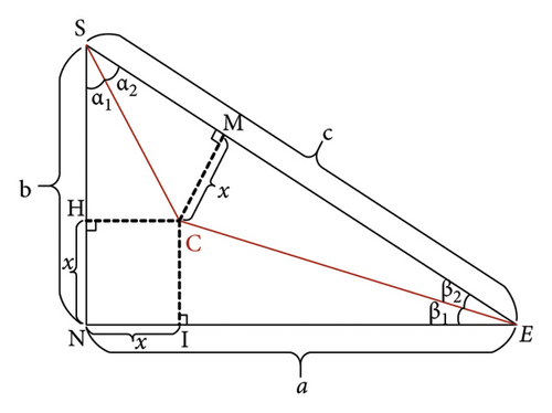
The h(n) uses circular arc distance in distance calculation and corrects it with projection distance, considering that the added cost of the two distances is slightly greater than the actual, and the dynamic weight is introduced to adjust the overall cost and to control the search speed of the algorithm.
Among them, Sc represents the arc distance, where the radius length is calculated by Sj and the Sj represents a combination of Manhattan distance (as b + a in Figure 1) and Euclidean distance (as c in Figure 1), and it represents the current distance based on the coordinate information of the starting and ending points. St represents the distance from the current point to the starting and ending points of the straight line. The calculation method for each distance is as follows.
3.1.2.1. Arc Distance
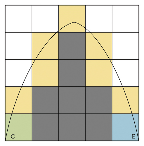
When estimating the distance cost in h(n), the closer to the actual distance, the better the algorithm is. However, the estimation of this distance in traditional algorithms often ignores the obstacles, so the estimated distance is often less than the actual distance. Therefore, considering the actual obstacles, as shown in Figure 2, the black grid represents the obstacle, C represents the current node, and N represents the end point. Given the most general situation of the obstacles, the distance between the current point and the end point is approximately half of the diameter circle with the distance between the current point and the end point, as shown in the arc CE.
3.1.2.2. The Distance Between the Current Point and the Straight Line
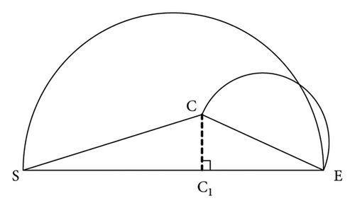
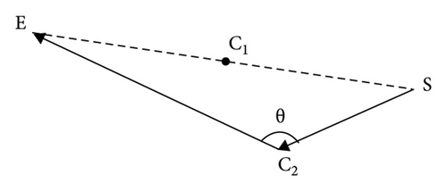
When the current point is in C, according to the calculation of the arc distance, CE is the diameter. At this time, the arc distance in (5) has been calculated in advance. If the current point of the path is selected at C1, the radius of the corresponding arc distance will change. Therefore, introduce the distance between the current point and the straight line, which reflects the deviation between the current point and the shortest route. The closer the distance to the current point, the less the offset representing the current point from the optimal route.
3.1.3. Weight Design
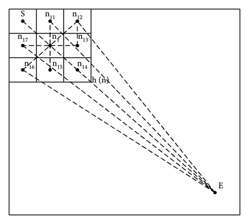
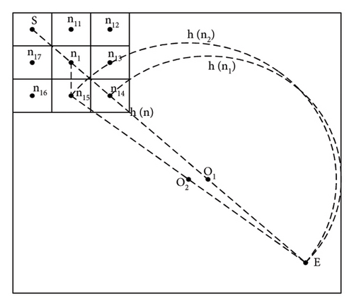
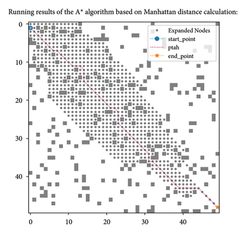
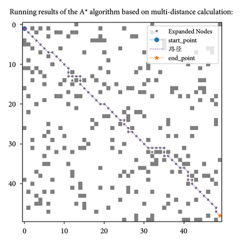
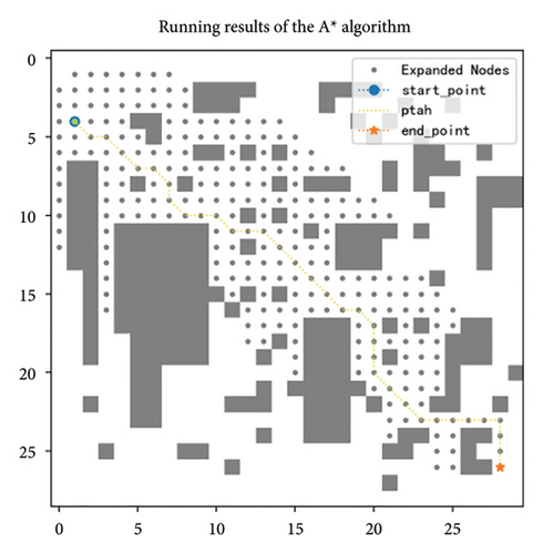
As shown in Figure 5(a), guided by the Euclidean distance as the heuristic function, with the starting point set as S and the ending point set as E. The current point extends from the starting point to n1. At this point, n1 needs to expand to the surrounding eight nodes and select the node with the lowest proxy value as the next expansion node. Taking the extension of n1 to n14 and n15 as an example, the total cost of extending the current point to n14 is the actual cost from S to n1 and then to n14, plus the Euclidean distance from n14 to endpoint E. Similarly, the total cost of extending the current point to n15 is the actual cost from S to n1 and then to n15, plus the Euclidean distance from n15 to E. Since both points n15 and n14 are adjacent to node n1, the difference in the cost values of the Euclidean distance between the two points and the endpoint E will be very small. Therefore, the sum of the actual cost and estimated cost, that is, the total cost, is very similar, and there may even be two minimum cost cases. The direction of extension is not unique. At this time, the A ∗ algorithm node extension extends to the endpoint according to the dashed area, which is roughly the two sides of the straight line formed by the starting point S and the endpoint E, and the area varies with the distribution of obstacles. There will be some adjustments. In Figure 5(b), the A ∗ algorithm is guided by the principle of multidistance heuristic function. When selecting the next extension node at the current point n1, the distance h(n) is multiplied by the weight of the arc distance, and the distance from the point to the line is added to the distance from the current point to the line SE. When the current point extends from n1 to n14, n14 is on the straight line SE, so the distance to the straight line SE is 0 and the weight value p is also 1. The estimated cost h(n1) is the length of the arc formed by the diameter from n14 to the endpoint E. The radius of the arc is calculated according to Figure 1, which is formula (3). Therefore, the total cost from n14 to the endpoint E is the length of the arc plus twice . Similarly, the total cost from n15 to the endpoint E is the corresponding arc distance h(n2) multiplied by the weight value plus , plus the distance from n15 point to the straight line SE. However, due to the significant difference in the calculation of arc distance, and n15 being near node n1, the weight value calculated according to formula (10) is also infinitely close to 1. With a small difference of about 0.4 in actual cost, the node with the smallest total substitution value will have a relatively unique situation, mainly expanding in the direction of the straight line formed from node S to the endpoint E. When encountering obstacles, the number of extensions will increase. Figures 5(c) and 5(d) show the path length and node expansion number of the algorithm using Euclidean distance and multidistance heuristic functions in the 50 × 50 size map, respectively. It can be intuitively seen that the search area and analysis direction of the algorithm are the same, proving the efficiency of the proposed multidistance heuristic function in search.
The impact of h(n) on algorithm performance is mainly reflected in the following aspects.
3.1.3.1. Quality of Path Search
When h(n) can accurately reflect the distance metric from the current node to the goal node, the search path generated by the A ∗ algorithm will be equivalent to or close to the global shortest path. Conversely, if there is bias in the estimated value of h(n), the algorithm may explore longer paths or even nonoptimal paths.
3.1.3.2. Efficiency of Path Search
The weight of h(n) also significantly affects the search speed of the algorithm. When the weight is large, the algorithm tends to quickly advance toward the endpoint, thereby accelerating the search speed, but may miss the optimal path as a result. On the contrary, if the weight of h(n) is small, the algorithm focuses more on finding the optimal path, which often leads to a slowdown in search speed.
In response to the issue mentioned in (1), this paper innovatively designs multiple distance functions, taking into account the situation where obstacles are dense, and builds an estimation value close to the actual cost. However, this estimation value may be slightly higher than the actual cost, so we introduce a weight to balance it. Specifically, the design of weight takes into account the relative positional relationships between the starting point, the endpoint, and the current node. This ensures the algorithm’s efficient search capability while balancing the overall cost estimation. The experimental results of path search in a 50 × 50 map environment are shown in Figure 5(e). The comparison shows that, using the Manhattan distance, the algorithm with the weight design proposed in this paper (Figure 5(e)) significantly reduces the number of nodes explored during the search process compared to the algorithm without weight design (Figure 5(c)), indicating that the weight design method proposed in this paper has certain advantages.
3.1.4. Repulsive Potential Field of Obstacles
The calculation formula of the repulsion potential field is the square of the inverse of the distance multiplied by the influence factor, where the influence factor β is 1, hre is the Euclidean distance between the current point and the nearest obstacle, threshold is the action threshold range of the obstacle, and the limited range is within 0–2. Within this range, the repulsion is generated. When the robot is very close to the obstacle, the overall cost function will increase sharply, and the repulsion factors exclude the corresponding nodes and turn to the nodes with fewer obstacles around it, making the robot have the consciousness to actively bypass the obstacles in the process of movement. Compared with the traditional A ∗ algorithm, the repulsion effect on the obstacles is added to the heuristic function, and the prior knowledge of the obstacles and the target point in the environment is effectively used. Under the influence of repulsion, the robot can effectively avoid obstacles and improve the safety of the path.
3.1.5. Turning Cost
In the traditional A ∗ algorithm, the path smoothness is sacrificed to obtain the shortest path. However, frequent steering can cause great damage to the logistics robot, and thus, increasing the cost of turning, this section aims to minimize the cost of path planning to the greatest extent possible. By calculating the angle between the parent node and the current point and converting it to the corresponding radian value. The robot produces a radian between the two steps, which transforms the radian into the corresponding turning generation value. Integrate the perspective change of the current point into the estimation value and consider the increase of the estimation value brought by the frequent turn in the cost. Frequent turns increase the cost, which will reduce the chance of choosing the node, and to some extent can minimize the turn, making the search path smoother. Pseudocode is shown in Algorithm 1.
-
Algorithm 1: Computes the turningcost.
-
Input: MinF (the current minimum node cost), offsetX (x direction offset), offset (y direction offset)
-
Output: turningcost
- 1.
Calculate the steering cost between two points (in radian)
- 2.
If minF.father then
- 3.
dx1 ⟵ minF.point.x - minF.father.point.x {calculate the X direction difference}
- 4.
dy1 ⟵ minF.point.y - minF.father.point.y {calculate Y direction difference}
- 5.
dx2 offsetX {set the X-direction offset}
- 6.
dy2 offsetY {set the Y-direction offset}
- 7.
calculate the angle between the two vectors using the fork and point products.
- 8.
crossproduct dx1 ∗dy2 - dx2 ∗dy1 {calculated fork product}
- 9.
dotproduct dx1 ∗dx2 + dy1 ∗dy2 {calculate dotproduct}
- 10.
calculate the radian angle
- 11.
angle abs (arctan2 (crossproduct, dotproduct)) {calculate the radian angle}
- 12.
turn the angle into the cost
- 13.
turningcost ⟵ angle ∗stepv {convert angle to. cost}
- 14.
end if
- 15.
return turningcost
3.2. Extension Node Selection Based on Simulated Annealing
The traditional A ∗ algorithm mainly estimates the cost of h(n). The cost of g(n) is calculated according to the number of steps and then choosing the node with the lowest estimation value by the sum of h(n) and g(n). In this process, a large number of nodes with estimation values may be generated. Therefore, the idea of simulated annealing is introduced, and the next node is selected according to the probability calculated by the estimation value at each step of node selection and can jump out of the local optimum in the traditional algorithm.
According to the basic principle of simulated annealing and the basic process of A ∗ algorithm, the process of designing extension nodes is shown below, where the magnitude of the energy is expressed as the estimated cost of the current node to the endpoint.
3.2.1. Initialization Parameters
Initial the temperature and the annealing rate. The initial value of the energy is the estimate of the heuristic function h(n) of the current point to the end point. Expand the initial nodes and update the open list and the close list. That is, put the starting node into the list and then start to expand the node according to the expansion direction of the five fields, and put the starting point and adjacent nodes into the open list set.
In the process of configuring the strategy that combines the simulated annealing algorithm with the A ∗ algorithm, the first step is to establish an appropriate initial temperature T and cooling rate r. To ensure that the algorithm can extensively explore the global space in the initial stage, the initial temperature T needs to be set high enough to increase the probability of accepting worse solutions. Specifically, this initial temperature should exceed the range of the search space, ensuring that the algorithm has strong exploratory capabilities at the beginning. However, an excessively high initial temperature will also correspondingly extend the algorithm’s operation cycle and increase computational costs. Given that the maximum size of the map in this paper is 200 × 200, the upper limit of the initial temperature is set to 300. At the same time, considering the impact of the initial temperature on the algorithm’s solution speed and that the energy value in the simulated annealing process of this paper is calculated based on the fitness value, with the difference in fitness values not exceeding three in each node selection step, the lower limit of the initial temperature is set to 3.
The cooling rate, which is the speed of the temperature decreases, significantly affects the performance of the algorithm. An overly fast cooling rate may cause the algorithm to converge to a local optimal solution too early, while an overly slow cooling rate will extend the algorithm’s running time, thereby increasing computational costs. Generally, the cooling rate is set between 0.8 and 0.99, which is both simple and practical, but may need to be adjusted according to specific problems. Given that the fitness value differences in this paper are small, several values such as 0.985, 0.98, and 0.9 are chosen for experimentation.
Analyzing the data in Table 1, it can be seen that the value of the cooling rate has a relatively small impact on the algorithm’s results. This is because the fitness value calculation in this paper is specific, and the cooling rate value is less than 1, which has a limited impact on the overall fitness value. Figure 6 intuitively shows the significant impact of different initial temperatures on the number of expanded nodes. When the initial temperature is high, the algorithm expands more nodes during operation. After numerous experiments and analyses, it is ultimately determined that the initial temperature for this paper is 3, and the cooling rate is 0.985.
| Parameter settings | Time | Node | Length |
|---|---|---|---|
| T = 300, r = 0.985 | 0.4562 | 176 | 71.2499 |
| T = 300, r = 0.98 | 0.3592 | 253 | 71.2499 |
| T = 300, r = 0.9 | 0.3158 | 228 | 71.4499 |
| T = 200, r = 0.985 | 0.1537 | 257 | 71.4499 |
| T = 200, r = 0.98 | 0.1380 | 213 | 71.4499 |
| T = 3, r = 0.985 | 0.1224 | 176 | 71.4499 |
3.2.2. Get a New Node n′
Select a new node n’ from the open list based on the estimated value f(n) of the node with the lowest value and calculate the energy of the new node n’ (i.e., the estimated value of n′).
3.2.3. Calculate the Increment
3.2.4. Judge Whether to Accept the Current Solution n′
3.2.5. Update Each Parameter
Update the annealing temperature T = T∗r based on the changes in the nodes. Expand the new node n’ and continuously update the open and close lists according to the five-neighborhood expansion method we adopted.
3.2.6. Termination Conditions
Repeat the previous step and terminate the iteration when the target node is in close list or the open list is empty (has gone through all traversal nodes), that is, find the target node or walk through all nodes without finding the optimal path.
3.3. A Bounded Suboptimal Value
In order to avoid the comparison of extended nodes with “low-cost performance” in the search process, the algorithm is more efficient through the design of ε value. In Table 2, the running time, extended node, and path length of the algorithm have the best running effect by taking ε as 0.2, that is, when the overall weight is 1.2. The selection of ε value in bounded suboptimal should be reasonably set according to the map, mainly focusing on the distribution of obstacles and targets. Based on the experimental comparison, it is generally appropriate to take the range of 0.1–0.5, because most of the repeated values appear in the range of 1.1–1.5 times the estimated value. If beyond this range, to twice the effect or more, it is difficult to find the right path.
| ε value | ε1 = 0.2 | ε2 = 0.05 | ε3 = 0.7 | ε4 = 1 |
|---|---|---|---|---|
| Performance period | 1.2317 | 1.8380 | 0.9135 | 1.7054 |
| Expanding node | 1458 | 1747 | 1235 | 1740 |
| Path length | 80.299 | 75.939 | 86.399 | 81.9399 |
3.4. Summary
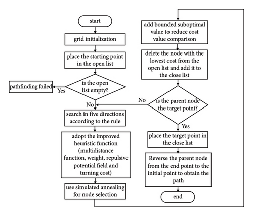
The improved A ∗ algorithm is reflected in the following aspects. Firstly, the heuristic function of the algorithm is improved by combining multiple distances and adding repulsive potential field, turning cost, and dynamic weight coefficient in the artificial potential field method. This process aims to make the estimated cost closer to the actual cost. Secondly, the idea of simulated annealing is introduced into node expansion selection to avoid getting stuck in local optima. In addition, the improved algorithm also adopts the five-neighborhood extension mode and the idea of bounded suboptimal to reduce unnecessary node extension and node estimation value comparison. The flowchart of the improved A ∗ algorithm is shown in Figure 7.
4. Removing Redundant Nodes
The improved algorithm proposed in this paper has made significant progress in reducing algorithm runtime and the number of node expansions, but the paths generated still contain some unnecessary turns. This phenomenon occurs partly because the heuristic function considers multiple factors such as turning costs, and the simulated annealing algorithm has a certain randomness in node selection, which cannot consider every node from a global perspective. Therefore, based on the improvement of the A ∗ algorithm, this paper introduces the Floyd algorithm to further smooth the path. The core principle of the Floyd algorithm is to adjust points or line segments in the path to reduce unnecessary twists and turns, thereby making the path smoother and more efficient.
-
Step 1. Redundant Node Identification.
-
Use the Floyd algorithm to calculate the shortest path from each node to its successor node in the path. If a node in the path is not a necessary node for the shortest path of its successor (i.e., the node is redundant), it can be removed from the path.
-
Step 2. Merging of Colocated Nodes.
-
In the path, if there are nodes with the same position (i.e., colocated nodes), these nodes are merged to reduce the total length of the path and enhance the smoothness of the path.
-
Step 3. Iterative Optimization Process.
-
Repeat the above two steps until there are no more redundant nodes that can be removed from the path.
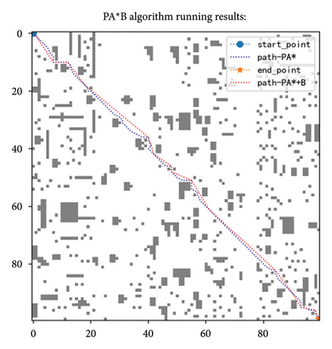
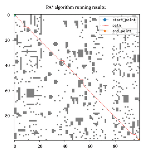
Through this method, the Floyd algorithm can effectively identify and remove redundant nodes in the path, simplify the path structure, and improve the smoothness of the path. Taking a 100-scale map as an example, the effect after removing redundant nodes is shown in Figure 8. Table 3 demonstrates the improvements achieved after removing redundant points, from which it is evident that the path length has been reduced. However, it is important to note that this optimization measure is a postprocessing step; hence, based on the PA ∗ algorithm, the required processing time has increased.
| Map | Algorithm | Time | Length | Algorithm | Time | Length |
|---|---|---|---|---|---|---|
| 30 | PA ∗ | 0.030 | 38.609 | PA ∗B | 0.041 | 37.549 |
| 35 | PA ∗ | 0.014 | 18.05 | PA ∗B | 0.056 | 18.05 |
| 40 | PA ∗ | 0.046 | 50.709 | PA ∗B | 0.127 | 48.624 |
| 50 | PA ∗ | 0.061 | 70.2699 | PA ∗B | 0.324 | 67.349 |
| 100 | PA ∗ | 0.585 | 135.4399 | PA ∗B | 1.152 | 131.179 |
| 200 | PA ∗ | 4.269 | 291.1300 | PA ∗B | 56.792 | 287.240 |
5. Algorithmic Simulation Experiments
5.1. Effectiveness of Single Strategy
To verify the feasibility of the proposed A ∗ algorithm (denoted as PA ∗), the effectiveness of each part in the PA ∗ algorithm, namely, the validation of the single strategy (Section 5.1), the validation of the overall strategy (Section 5.2), and the comparison with the existing algorithm (Section 5.3), is conducted in this section. All the above comparisons were made on six grid maps, including 30 × 30, 35 × 35, 40 × 40, 50 × 50, 100 × 100, and 200 × 200. Use Intel (R) Core (TM) i5-8250U CPU @ 1.80 GHz, 8 GB of running memory and PyCharm2020.1 for experimental hardware and software, respectively. The simulation running experiment is carried out by using Python3.0 programming in the PyCharm 2020 programming environment. The parameter settings of the proposed algorithm are shown in Table 4.
| The parameter name | Set up the situation |
|---|---|
| Action threshold range of the obstacle | threshold = 2 |
| The repulsive potential field influence factor | β = 1 |
| Initialize the temperature | T = 3 |
| The annealing rate | r = 0.985 |
| Boundary suboptimal | ε = 0.2 |
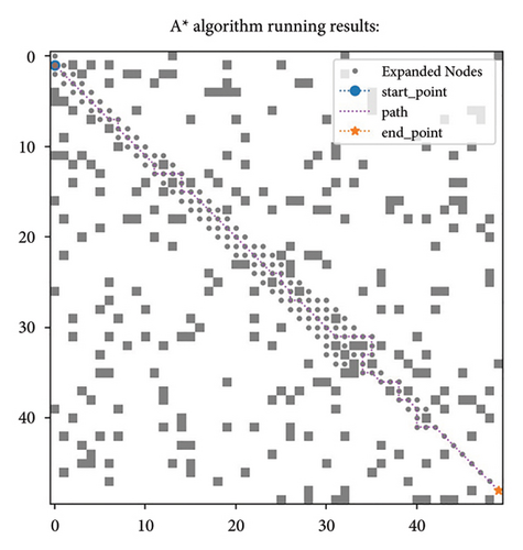
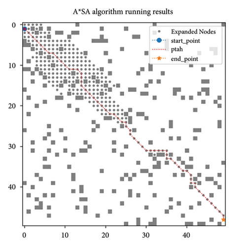
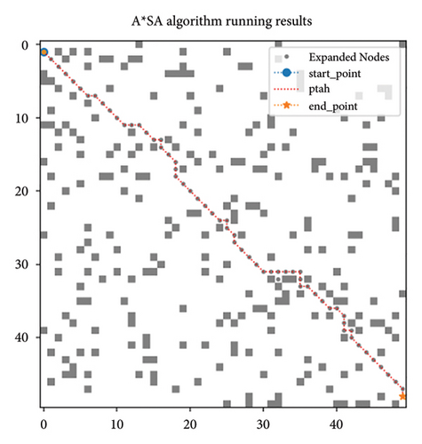
In this section, the basic algorithm (denoted as A ∗), the basic algorithm with simulated annealing strategy (denoted as A ∗SA), and the basic algorithm with modification heuristic function (denoted as A ∗IF) are compared in terms of the algorithm running time, extension node, and path length. The results are shown in Table 5.
| Map | Algorithm | Time | Panel point | Length |
|---|---|---|---|---|
| 30 × 30 | A ∗ | 0.0439 | 257 | 40.15 |
| A ∗SA | 0.0049 | 36 | 41.5599 | |
| A ∗IF | 0.0312 | 38 | 42.7399 | |
| 35 × 35 | A ∗ | 0.0396 | 95 | 18.64 |
| A ∗SA | 0.0019 | 27 | 18.64 | |
| A ∗IF | 0.0149 | 18 | 18.64 | |
| 40 × 40 | A ∗ | 0.2074 | 619 | 54.0199 |
| A ∗SA | 0.0079 | 49 | 54.2499 | |
| A ∗IF | 0.0089 | 46 | 54.02499 | |
| 50 × 50 | A ∗ | 0.3610 | 747 | 72.9899 |
| A ∗SA | 0.0109 | 62 | 74.7599 | |
| A ∗IF | 0.0625 | 64 | 75.3499 | |
| 100 × 100 | A ∗ | 5.7496 | 3142 | 138.7499 |
| A ∗SA | 0.0428 | 125 | 144.6499 | |
| A ∗IF | 0.5936 | 114 | 141.5699 | |
| 200 × 200 | A ∗ | 120.456 | 13711 | 300.2400 |
| A ∗SA | 1.1476 | 246 | 292.4907 | |
| A ∗IF | 4.2764 | 251 | 311.0900 | |
It can be seen from Table 5, the simulated annealing strategy greatly reduces the number of iterations, so select fewer nodes for comparison, which greatly reduces the running time of the algorithm on average by 95%, especially in large maps such as 100 × 100 and 200 × 200 specifications as shown in Figure 9, the running time is reduced by about 99%. However, for the small maps as 30 × 30, 40 × 40, and 50 × 50, the path length increases by 0.24%–3.511%, the slight increase in path length in the minimap is mainly because the high early temperature in the simulated annealing process can accept the principle of gradient descent locally a certain probability. But as the temperature gradually decreases, the probability of this acceptance decreases to almost zero. The path length becomes shorter on the 200 × 200 map. This is mainly because after the introduction of simulated annealing ideas, the whole path search process will jump out of the shock within the local range of the traditional algorithm and directly show the trend of searching from the current point to the end point.
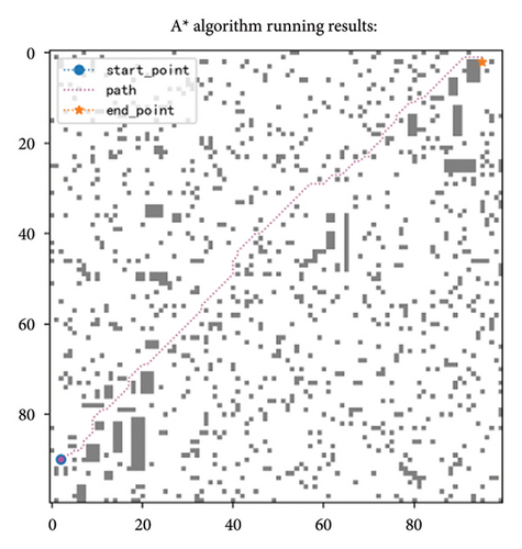
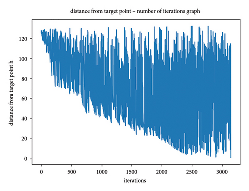
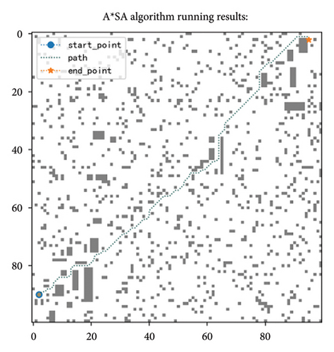
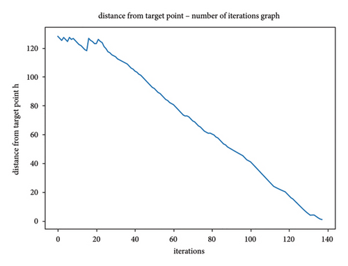

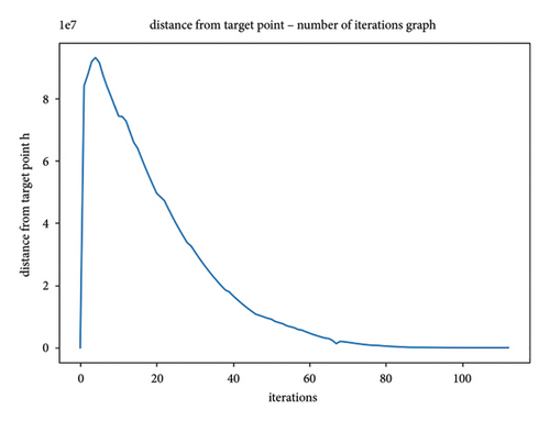
For the traditional algorithm with modified heuristic function, using multiple distance-inspired functions, six specification maps are less than the traditional algorithm of nodes, the average node increase efficiency is 89%, but the path length except 35 × 35 map 0.009%–6.45% increases, about 3%, because the average increase more distance-inspired function slightly greater than the actual value on valuation, so will expand less nodes. Meanwhile, the time to the endpoint is reduced, with an average reduction of 75%.
5.2. Validation of the Overall Strategy Effectiveness
This section verifies the effectiveness of the proposed strategy fusion, that is, whether the proposed strategy fusion has an impact on the overall performance. This section compares the performance of three algorithms: the whole fusion algorithm (PA ∗), the algorithm PA ∗ removing modified heuristic function (PA ∗-IF), and the algorithm PA ∗ removing simulated annealing strategy (PA ∗-SA). The results are shown in Table 6.
| Map | Algorithm | Time | Expand node | Length |
|---|---|---|---|---|
| 30 × 30 | A ∗ | 0.043 | 257 | 40.15 |
| PA ∗ | 0.030 | 30 | 38.609 | |
| PA ∗-IF | 0.030 | 47 | 40.379 | |
| PA ∗-SA | 0.033 | 80 | 38.609 | |
| 35 × 35 | A ∗ | 0.039 | 95 | 18.64 |
| PA ∗ | 0.014 | 16 | 18.05 | |
| PA ∗-IF | 0.024 | 52 | 23.69 | |
| PA ∗-SA | 0.022 | 25 | 18.05 | |
| 40 × 40 | A ∗ | 0.207 | 619 | 54.0199 |
| PA ∗ | 0.046 | 38 | 50.709 | |
| PA ∗-IF | 0.057 | 61 | 64.609 | |
| PA ∗-SA | 0.062 | 117 | 50.7099 | |
| 50 × 50 | A ∗ | 0.361 | 747 | 72.9899 |
| PA ∗ | 0.061 | 51 | 70.2699 | |
| PA ∗-IF | 0.101 | 84 | 81.8099 | |
| PA ∗-SA | 0.090 | 162 | 70.2699 | |
| 100 × 100 | A ∗ | 5.749 | 3142 | 138.7499 |
| PA ∗ | 0.585 | 101 | 135.4399 | |
| PA ∗-IF | 0.595 | 135 | 149.9299 | |
| PA ∗-SA | 0.764 | 310 | 135.4399 | |
| 200 × 200 | A ∗ | 120.45 | 13,711 | 300.2400 |
| PA ∗ | 4.269 | 212 | 291.1300 | |
| PA ∗-IF | 5.201 | 374 | 343.2900 | |
| PA ∗-SA | 4.458 | 214 | 291.1300 | |
- Note: Bold values indicate the best value of the corresponding variable in several methods.
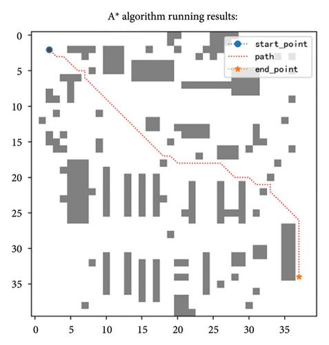
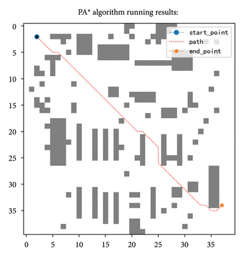
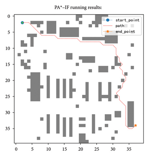
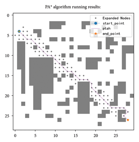
According to Table 6, the PA ∗ algorithm achieved the corresponding improvements in running time, extended nodes, and path length, in which the running time decreased by 73%, the number of nodes reduced by 92%, and the path shortened by about 3.7% compared with A ∗. Compared with the fusion strategy, the original heuristic function (i.e., PA ∗-IF) in the fusion strategy has worse effect. In Figures 10(a) and 10(c), we can intuitively see that on the 40 × 40 specification map, the path obtained by the fusion strategy is more tortuous and the path is longer. At the same time, the running time of the extended node and the algorithm increased, the extended node increased by 48%, the running time increased by 30%, and the path length increased by about 18%. If the simulated annealing is removed from the fusion strategy, the length of the path is not affected, as shown in Figures 10(b) and 10(d), but the algorithm running time and expansion nodes are still more than the fusion strategy and the average algorithm running time is about 31.7%, while the expansion node is 1.4 times more on average. Through comparison, it is not difficult to see that if only a single strategy is adopted, the effect is not as good as the strategy integration. This also proves from the side that the proposed improvement can achieve the balance of the algorithm and can get the optimal effect to the maximum extent, so it shows that the overall improvement method is effective.

5.3. Comparison With the Existing Improved A ∗ Algorithms
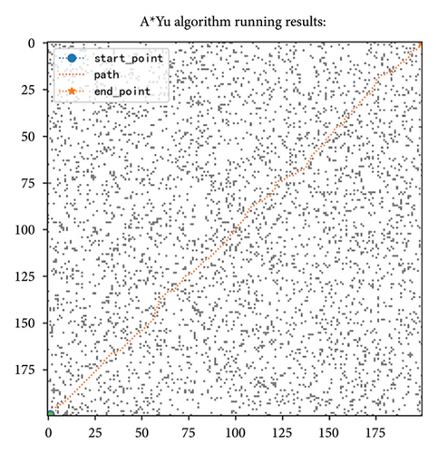
This section verifies the advancement of the PA ∗ algorithm by comparing the algorithms with the existing literature. The comparison algorithms are as follows. The improved A ∗ algorithm proposed by Xu, Li, and Fei [33] is recorded as the A ∗Xu. The improvement algorithm proposed by Yu et al. [42] is based on the weighted average distance and weights considering the proportion of obstacles, denoted as the A ∗Yu. The A ∗ algorithm based on jump point search proposed by Yao et al. [40] is classified as A ∗JPS. The comparison results are shown in Table 7. In Table 7, the best result is bold display, and in the time column, the best and second best are both displayed in bold. It can be found that the PA ∗ algorithm performed the best in term of the expand nodes and the length. In the time aspect, the PA ∗ algorithm performed second best and did not differ significantly from the first place of A ∗Yu. The improvement of the heuristic function by Yu et al. includes the weighted average distance and the weight design according to the obstacle, greatly shortening the corresponding time of the algorithm, with the average time reduction of 55% compared to the PA ∗ algorithm in this paper. This is mainly because the power function with e as the base in the weight design makes the estimation function weight very large, and the algorithm will search the map very quickly. However, this also often leads to the resulting path is not optimal, so only to improve the time index, the resulting path length will be larger than the optimal path.
| Map | Algorithm | Time | Expand nodes | Length |
|---|---|---|---|---|
| 30 × 30 | A ∗ | 0.044 | 257 | 40.150 |
| PA ∗ | 0.031 | 30 | 38.610 | |
| A ∗Xu | 0.050 | 217 | 39.493 | |
| A ∗JPS | 0.581 | 88 | 37.870 | |
| A ∗Yu | 0.028 | 53 | 38.409 | |
| 35 × 35 | A ∗ | 0.040 | 95 | 18.64 |
| PA ∗ | 0.014 | 16 | 18.05 | |
| A ∗Xu | 0.046 | 218 | 18.305 | |
| A ∗JPS | 0.153 | 10 | 18.071 | |
| A ∗Yu | 0.008 | 19 | 17.904 | |
| 40 × 40 | A ∗ | 0.207 | 619 | 54.020 |
| PA ∗ | 0.046 | 38 | 50.710 | |
| A ∗Xu | 0.217 | 282 | 52.368 | |
| A ∗JPS | 0.5227 | 85 | 52.355 | |
| A ∗Yu | 0.008 | 52 | 51.878 | |
| 50 × 50 | A ∗ | 0.3610 | 747 | 72.990 |
| PA ∗ | 0.0619 | 51 | 70.270 | |
| A ∗Xu | 0.1856 | 256 | 70.936 | |
| A ∗JPS | 1.2206 | 230 | 73.740 | |
| A ∗Yu | 0.0129 | 68 | 70.897 | |
| 100 × 100 | A ∗ | 5.7496 | 3142 | 138.750 |
| PA ∗ | 0.5854 | 101 | 135.440 | |
| A ∗Xu | 2.7451 | 1167 | 137.025 | |
| A ∗JPS | 3.6454 | 760 | 137.575 | |
| A ∗Yu | 0.3168 | 121 | 138.670 | |
| 200 × 200 | A ∗ | 120.456 | 13,711 | 300.240 |
| PA ∗ | 4.2695 | 212 | 291.130 | |
| A ∗Xu | 21.7560 | 4006 | 293.692 | |
| A ∗JPS | 17.4920 | 3009 | 283.043 | |
| A ∗Yu | 1.6424 | 276 | 289.109 | |
- Note: Bold values indicate the best value of the corresponding variable in several methods.
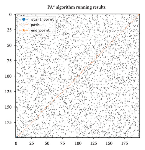
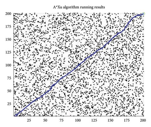
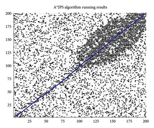
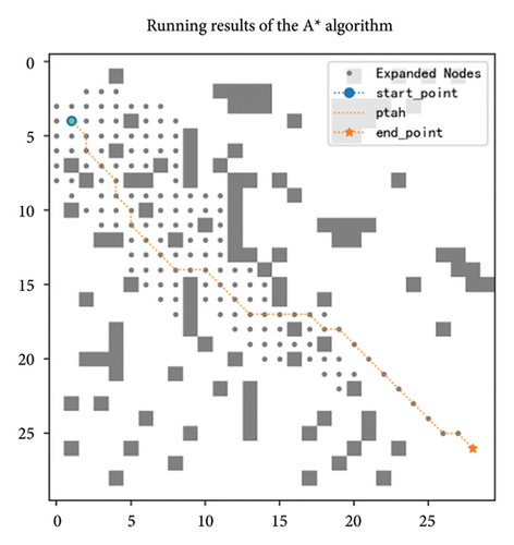
By analyzing the data of Table 7, compared with the traditional algorithm A ∗, the average running time of PA ∗ is decreased by more than 70%, the number of expanded nodes is reduced by 92%, and the path length is reduced by about 3%. In A ∗Xu, a redundant point deletion and deleted unnecessary node strategy were proposed, which reduced the extended nodes and path length, compared with the traditional algorithm A ∗. However, the PA ∗ algorithm greatly reduces the number of extended nodes and the path time compared with A ∗Xu. The PA ∗ algorithm is reduced by 1.6% in term of the path length, the time by 68%, and the extended nodes by 88% compared with A ∗Xu. This is mainly because the A ∗Xu algorithm added dynamic weight based on the current point position, but the weight value is small, and because the distance function is too large, so there is still a big gap between the weight and the actual cost. As shown in Figure 11(b), in the early stage, because of the small weight, the estimated value of the heuristic function was much smaller than the actual value, so the algorithm searched for a large number of nodes, and the efficiency was very low. However, when the current point gradually approaches the end point, the larger weight makes the estimated value gradually approach the actual value, and the algorithm only needs to search for fewer nodes. Jump point search by predicting the target direction to jump out of the useless search space, although can quickly find a feasible path, but also will miss some path, cannot guarantee the path is global optimal, so compared to the improved algorithm, path length increased by about 1%, and time will increase by 10.8%, and the number of extension nodes also increased by 4% on average, as shown in Figure 11(c). The A ∗ JPS algorithm still expands more nodes in search near the endpoint, which is not as good as the PA ∗ algorithm traversing very few nodes at this time. In comparison, the improved algorithm in this paper fits the global optimal path, and because of the design of the distance function and the node selection mode of the simulated annealing, the algorithm running time and the extended nodes are basically the least, which is more efficient than the algorithm proposed in the existing literature.
5.4. Comparison With Other Types of Algorithms
5.4.1. Compared With ACO
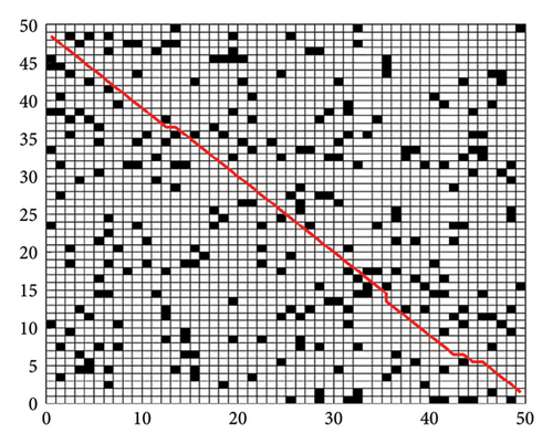
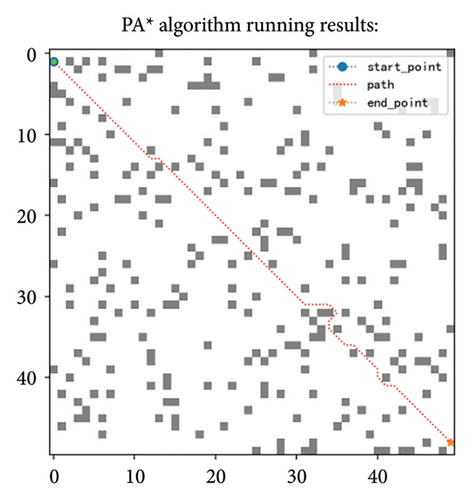
Comparing the improved algorithm with the ACO [2] algorithm, and from Figure 12 and Table 8, we can draw the following conclusions. From the perspective of path length, the path planned by the ACO algorithm is slightly shorter than that of the improved algorithm proposed in this paper. However, when evaluating algorithm performance, we must consider not only the single indicator of path length but also other important factors such as time efficiency.
| Map | Time | Length |
|---|---|---|
| 30 × 30 | 94 | 37.8701 |
| 35 × 35 | 97 | 18.0711 |
| 40 × 40 | 321 | 50.8406 |
| 50 × 50 | 803 | 69.0538 |
| 100 × 100 | 7660 | 133.3797 |
| 200 × 200 | 25,300 | 287.2745 |
In terms of time cost, the ACO algorithm consumes a significant amount of time during the pathfinding process, especially when dealing with large-scale maps, where this time cost exhibits an exponential growth trend. This means that as the map size increases, the running time of the ACO algorithm will increase dramatically, thereby limiting its feasibility in practical applications.
In contrast, although the improved algorithm in this paper may be slightly inferior to the ACO algorithm in terms of path length, its advantage in time efficiency is very obvious. The improved algorithm can complete path planning in a relatively short time, especially when dealing with large-scale maps, where the growth rate of time cost is much lower than that of the ACO algorithm. This advantage makes the improved algorithm more practical and widely applicable in practical applications. Therefore, considering both path length and time efficiency, we can conclude that the improved algorithm in this paper has an overall advantage and will perform better in practical applications. This conclusion not only validates the effectiveness of the improved algorithm but also provides strong support for its application in related fields.
5.4.2. Compared With Theta ∗ and D ∗Lite
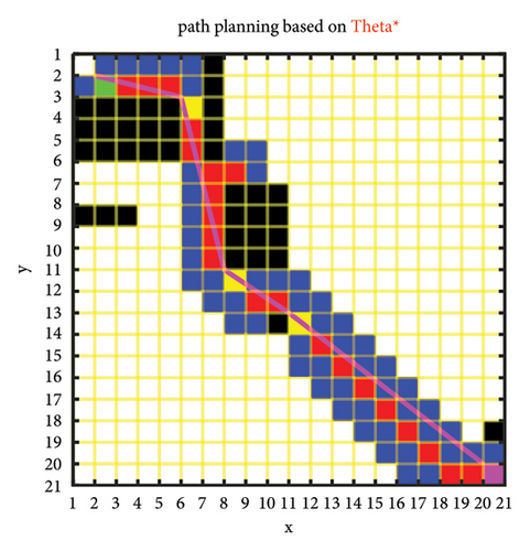
The Theta ∗ algorithm [43] integrates the heuristic characteristics of the A ∗ algorithm with the dynamic programming advantages of the Theta algorithm, expanding nodes only when they are crucial for finding better paths, thereby reducing computational costs and improving efficiency. Moreover, the Theta ∗ algorithm can handle any angle during the path search process, not limited to the traditional eight basic directions. The D ∗Lite algorithm [44], on the other hand, is an incremental search path-planning algorithm specifically designed for dynamic environments; it avoids the recalculation of the global path by locally updating the path information affected by environmental changes and employs a strategy of searching backward from the goal point to the starting point.
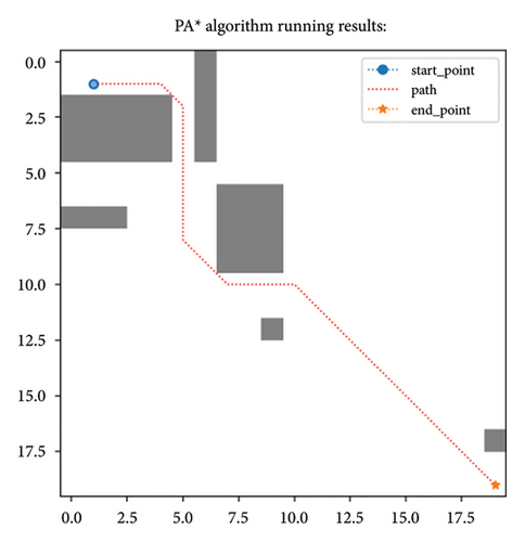
As shown in Figure 13(a), the pink squares represent key grids, with yellow cells indicating the grids that the final path must pass through. By comparing the improved algorithm proposed in this paper shown in Figure 13(b), the algorithm takes 0.009 s and expands 25 nodes, and the path length is 28.92. The Lazy Theta ∗ algorithm’s path length is approximately 27.81, with a runtime of 1.0140 s. The Theta ∗ algorithm can handle searches at any angle, thus resulting in shorter paths.
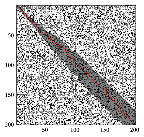
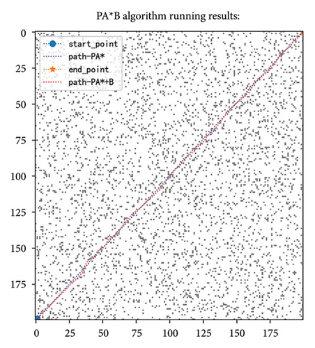
On a 200-scale map, as shown in Figures 13(c) and 13(d), after redundant node removal, the improved algorithm in this paper has a path length of 300.4 and expands 1847 nodes. In comparison, the D ∗Lite algorithm expands 4364 nodes with a path length of 298.531. Overall, the path lengths of the two algorithms are very close, indicating that the improved algorithm in this paper is superior in performance. Although slightly inferior to the D ∗Lite algorithm in terms of path length, the improved algorithm in this paper performs better in terms of node expansion and algorithm runtime. The Theta ∗ algorithm and D ∗Lite algorithm are more suitable due to its adaptability in dynamic environments. Moreover, considering the high density and disordered distribution of random obstacles, as depicted in Figure 5(d), the Theta ∗ algorithm must conduct a thorough evaluation of node selection and elimination when planning a path in such a complex environment. In contrast, the enhanced algorithm proposed in this paper spends less time during the node expansion phase, and after the removal of redundant nodes, it achieves results that are comparable to those of the Theta ∗ algorithm.
In summary, the improved algorithm in this paper shows significant advantages in efficiency and resource consumption, especially in path planning for large-scale maps. Although slightly less precise in path optimization compared to the Theta ∗ algorithm and D ∗Lite algorithm, its optimization in node expansion and computation time makes it a more efficient and practical pathfinding method for practical applications. With the advancement of technology and further development of algorithms, we look forward to these algorithms providing more accurate and efficient path-planning solutions in dynamic and complex environments.
5.5. PA ∗ Algorithm Comparison in Different Obstacle Densities
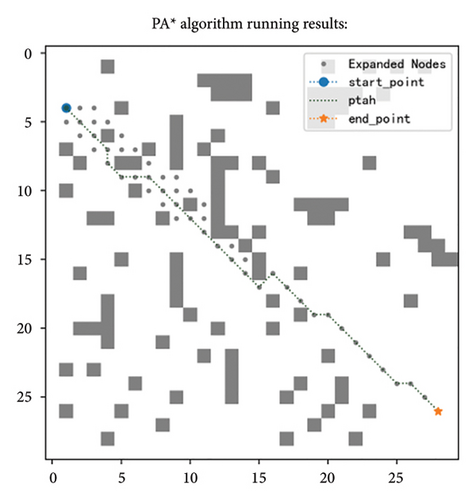
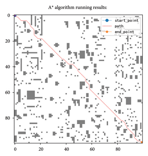
According to Table 9 and Figure 14, the improved algorithm outperforms the basic algorithm under different obstacle ratios, which to some extent validates the universal applicability of the algorithm. Specifically, whether in environments with varying obstacle ratios or under different map sizes, the average running time of the basic A ∗ algorithm reached 2.2152 s, while the improved algorithm only required an average of 0.7 s. Observing from the perspective of the number of expanded nodes, the basic algorithm produced approximately six times as many nodes as the improved algorithm. Moreover, the path length generated by the improved A ∗ algorithm is also shorter than that of the basic algorithm, and this advantage becomes increasingly significant as the scale of the map expands.
| Map | Algorithm | Proportion of obstacles | Time | Expand nodes | Length |
|---|---|---|---|---|---|
| 50 × 50 | A ∗ | 0.11 | 0.1302 | 150 | 37.7899 |
| 50 × 50 | PA ∗ | 0.11 | 0.015074 | 30 | 37.4299 |
| 50 × 50 | A ∗ | 0.25 | 0.3063 | 257 | 40.15 |
| 50 × 50 | PA ∗ | 0.25 | 0.046305 | 91 | 38.6099 |
| 100 × 100 | A ∗ | 0.13 | 3.1130 | 2281 | 148.4399 |
| 100 × 100 | PA ∗ | 0.13 | 1.2470 | 436 | 147.1299 |
| 100 × 100 | A ∗ | 0.098 | 5.3112 | 2934 | 148.0299 |
| 100 × 100 | PA ∗ | 0.098 | 0.8484 | 372 | 135.4399 |
5.6. Statistical Analysis Test
A comprehensive statistical comparison and analysis were conducted between the basic A ∗ algorithm and the improved algorithm PA ∗ proposed in this paper, as shown in Table 10. The experimental data clearly reveal the performance differences between the two algorithms across various evaluation dimensions.
| Group | Column count. | Time | Expand node | Length |
|---|---|---|---|---|
| PA ∗ | 6 | 0.83 ± 1.70 | 74.67 ± 73.34 | 100.70 ± 101.57 |
| A ∗ | 6 | 21.14 ± 48.70 | 3095.17 ± 5317.89 | 104.13 ± 104.44 |
| T value | −1.021 | −1.391 | −0.058 | |
| p value | 0.037 | 0.040 | 0.959 | |
Regarding the key metric of “time,” the average time consumption of PA ∗ was 0.83 ± 1.70, significantly lower than that of the A algorithm, which was 21.14 ± 48.70. A t-test (with a T value of −1.021 and a p value of 0.037) confirmed that PA has a significant advantage over A in terms of runtime.
In terms of the “expand node” metric, PA ∗′s average number of node expansions was 74.67 ± 73.34, also significantly lower than A ∗’s 3095.17 ± 5317.89. The results of the t-test (with a T value of −1.391 and a p value of 0.040) further corroborate the superior performance of PA ∗ in node expansion efficiency.
As for the “length” metric, the performance of the two algorithms was relatively close. The average path lengths for PA and A were 100.70 ± 101.57 and 104.13 ± 104.44, respectively. The t-test results (with a T value of −0.058 and a p value of 0.959) indicated that the difference in path length between the two algorithms was not significant. Nonetheless, PA still demonstrated a slight optimization in path length.
In summary, PA ∗ algorithm showed significant advantages over A ∗ algorithm in both runtime and node expansion efficiency. Similarly, when PA ∗ was compared with other algorithms such as A ∗JPS, the improved algorithm PA ∗ proposed in this paper exhibited better performance overall. This fully substantiates the statistical significance of PA ∗ in reducing runtime and enhancing node expansion efficiency. Although the optimization effect on the path length metric was not significant, there was still a certain trend of improvement.
6. Conclusion
This paper develops a multidistance heuristic function, incorporating dynamic weights, repulsive potential fields, and turning costs into the heuristic function. The concept of bounded suboptimal correlation and a simulated annealing strategy are adopted to improve the traditional A ∗ algorithm in node selection. Compared with traditional algorithms, the proposed algorithm reduces the average running time by more than 70%, cuts the number of expanded nodes by 92%, and also shortens the path. After removing the redundant points from the path, the resulting path not only becomes smoother and more fluid but also experiences a further reduction in length. Compared with other existing algorithms, our approach is more efficient in terms of running time, expanding nodes, and path length, thereby validating the effectiveness of our improved algorithm. The improved A ∗ algorithm holds significant importance in the fields of robotics, game development, and autonomous driving vehicles. In the realm of robotics, it optimizes path planning, enhancing the efficiency and safety of robots navigating complex environments. In game development, the algorithm makes nonplayer character behavior more intelligent and natural, optimizes map generation and exploration processes, and aids in achieving dynamic difficulty adjustments, thereby enhancing the player experience. For autonomous driving vehicles, the improved A ∗ algorithm not only increases driving safety and efficiency but also quickly adapts to complex traffic environments, ensuring the safe operation of the vehicle. Future research on the A ∗ algorithm will focus not only on strategies to enhance node count, running time, and path length but also on integrating the A ∗ algorithm with local path-planning techniques, allowing the algorithm to navigate around obstacles based on global path planning.
Conflicts of Interest
The authors declare no conflicts of interest.
Funding
This work has been supported by the Fujian Provincial Natural Science Foundation Projects under Grant No. 2024J01833, in part by the Education and Research Projects for Middle and Young Teachers (Science and Technology) of Fujian Provincial under Grant No. JAT231057, in part by the Scientific Research Foundation of Fujian University of Technology under Grant Nos. GY-Z220295 and GY-Z22071, and in part by the third batch of Innovative Star Talent Project in Fujian Province under Grant No. 2023002.
Acknowledgments
We would like to express our gratitude to Professor Ding Jinliang from Northeastern University (China), for his strict supervision of the structure and content of the paper, and for providing many constructive suggestions.
Open Research
Data Availability Statement
The data that support the findings of this study are available from the corresponding author upon reasonable request.


