MCOA: A Multistrategy Collaborative Enhanced Crayfish Optimization Algorithm for Engineering Design and UAV Path Planning
Abstract
The crayfish optimization algorithm (COA) is a recent bionic optimization technique that mimics the summer sheltering, foraging, and competitive behaviors of crayfish. Although COA has outperformed some classical metaheuristic (MH) algorithms in preliminary studies, it still manifests the shortcomings of falling into local optimal stagnation, slow convergence speed, and exploration–exploitation imbalance in addressing intractable optimization problems. To alleviate these limitations, this study introduces a novel modified crayfish optimization algorithm with multiple search strategies, abbreviated as MCOA. First, specular reflection learning is implemented in the initial iterations to enrich population diversity and broaden the search scope. Then, the location update equation in the exploration procedure of COA is supplanted by the expanded exploration strategy adopted from Aquila optimizer (AO), endowing the proposed algorithm with a more efficient exploration power. Subsequently, the motion characteristics inherent to Lévy flight are embedded into local exploitation to aid the search agent in converging more efficiently toward the global optimum. Finally, a vertical crossover operator is meticulously designed to prevent trapping in local optima and to balance exploration and exploitation more robustly. The proposed MCOA is compared against twelve advanced optimization algorithms and nine similar improved variants on the IEEE CEC2005, CEC2019, and CEC2022 test sets. The experimental results demonstrate the reliable optimization capability of MCOA, which separately achieves the minimum Friedman average ranking values of 1.1304, 1.7000, and 1.3333 on the three test benchmarks. In most test cases, MCOA can outperform other comparison methods regarding solution accuracy, convergence speed, and stability. The practicality of MCOA has been further corroborated through its application to seven engineering design issues and unmanned aerial vehicle (UAV) path planning tasks in complex three-dimensional environments. Our findings underscore the competitive edge and potential of MCOA for real-world engineering applications. The source code for MCOA can be accessed at https://doi.org/10.24433/CO.5400731.v1.
1. Introduction
Optimization pertains to determining the optimal solution for a given problem under certain constraints [1]. Concomitant with the technological revolution and advancements driven by artificial intelligence, optimization problems are emerging in various research domains, rendering the question of how to address these problems efficiently a subject of ardent discourse among scholars [2, 3]. Currently, existing optimization techniques can be classified into traditional methods and metaheuristic (MH) algorithms [4]. Traditional methods primarily utilize specific mathematical rules, such as gradient descent, quasi-Newton techniques, and Levenberg–Marquardt [5]. These methods necessitate gradient information and invariably produce the same solution once an input is given, so they are only suitable for solving some small-scale optimization problems at a theoretical level [6]. Nevertheless, the complexity of real-world engineering optimization problems is escalating, manifesting nondifferentiable, discontinuous, and nonlinear characteristics [7]. This results in traditional methods being almost powerless when confronted with such challenges. As research deepens, a gradient-free, problem-independent, and efficient stochastic optimization technique, namely, the MH algorithm, has garnered prominent attention, which is capable of finding optimal or near-optimal solutions for highly complicated nonlinear optimization problems within a rational time frame [8]. Besides, the MH algorithm possesses the advantages of simple structure, good adaptability, and robust local optimum avoidance [9]. Consequently, they are regarded as an ideal alternative to traditional methods and are becoming increasingly prevalent in scientific and engineering applications.
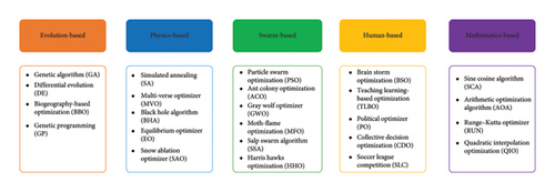
MH algorithms are inspired by natural phenomena, physical laws, or collective behaviors, and they can be grouped into five main categories [10]: evolutionary, physical, swarm-based, human-based, and mathematics-based algorithms, as shown in Figure 1. Evolutionary algorithms, like genetic algorithm (GA) [11], have a protracted development history and focus on natural selection and genetics. Physics-based algorithms derive their inspiration from chemical reaction processes and physical phenomena such as magnetism, attraction, and gravity. One well-known instance is simulated annealing (SA) [12], inspired by the principles of metallurgical annealing, which directs the convergence of the initial solution toward the global optimum according to the temperature distribution. The third category relates to the collective behaviors of birds, insects, animals, and other natural organisms referred to as swarm-based algorithms. Particle swarm optimization (PSO) [13] is a famous swarm-based optimization paradigm, which iteratively updates candidate solutions by emulating the foraging behavior observed in bird flocks. These algorithms are highly successful due to their ability to balance exploration and exploitation, allowing for efficient search across complex solution spaces. They are adaptable to various problem types, computationally efficient, and robust against local optima, making them reliable for diverse optimization tasks. Additionally, their self-organizing nature enhances their ability to handle distributed and dynamic environments. Human-based algorithms, including brain storm optimization (BSO) [14], are inspired by human social behavior, and mathematics-based algorithms, like sine cosine algorithm (SCA) [15], leverage mathematical principles for optimization.
- 1.
COA encompasses two exploitation phases, undermining its exploration capability. In the early iterations, COA maintains a high propensity to exploit, allowing for rapid convergence. Nonetheless, in later iterations, the exploration performance of COA is relatively feeble, making it susceptible to becoming trapped in local optima, thereby yielding suboptimal results. Consequently, there is a need to improve COA by adopting multiple strategies to establish a better exploration–exploitation balance and enhance stability so that it can cope with higher complexity and high-dimensional engineering optimization challenges.
- 2.
As the dimensionality and nonlinear constraints escalate, MH algorithms manifest a prevalent tendency of sluggish convergence and unsatisfactory solution accuracy for engineering optimization. While introducing a search operator can somewhat enhance the algorithm’s performance, it may indirectly impair its search capability in other facets. Therefore, multiple strategies can be adopted to synergistically reinforce the performance of MH algorithms from different aspects to confront complex optimization problems.
- 3.
According to the no free lunch (NFL) theorem [21], no single algorithm can guarantee the optimal solution for all optimization problems. Continuous development and enhancement of MH algorithms are necessary to provide more effective solutions for engineering optimization problems.
- •
We propose MCOA that integrates four improvement strategies: specular reflection learning for broader search, expanded exploration mechanism for enhanced global exploration, Lévy flight for efficient local search, and vertical crossover operator that helps stagnant individuals escape local optima.
- •
The performance of MCOA is comprehensively evaluated on 23 benchmark functions and the CEC2019/2022 test sets, comparing it with state-of-the-art MH algorithms across different dimensions (D = 50, 100, 500, 1000) to demonstrate its scalability.
- •
The applicability of MCOA is validated through seven constrained engineering design problems and UAV path planning cases, with experimental results confirming its superior convergence accuracy and stability even when facing highly complex optimization challenges.
The structure of this paper is as follows. Section 2 presents a literature review. Section 3 outlines the mathematical model of COA and the principles of the four improvement strategies. In Section 4, a detailed description of the proposed MCOA is provided, and its time complexity is analyzed. Section 5 compares the numerical optimization performance of MCOA with various well-established optimizers. MCOA is applied to address engineering design and UAV path planning problems in Section 6. Section 7 concludes this study.
2. Literature Review
Exploration and exploitation are indispensable components of MH algorithms. Exploration aims to comprehensively search the problem domain to uncover superior candidate solutions, while exploitation executes local searches within identified promising regions to converge toward the global optimum. Maintaining an appropriate balance between exploitation and exploration is crucial for an optimizer, as it directly determines its optimization performance. Notwithstanding the excellent flexibility and viability exhibited by MH algorithms in addressing optimization projects, due to the increasing complexity of emerging challenges in various fields, MH algorithms are inevitably susceptible to deficiencies such as sluggish convergence speed, suboptimal solution accuracy, and the propensity to become trapped in local optima [22]. The same is true for COA. Therefore, further enhancements to the original algorithm’s search performance are requisite. Wang et al. [23] proposed an improved multistrategy COA (IMCOA), which integrates the cave candidate strategy, fitness–distance balance competition strategy, optimal nondominance search strategy, and food covariance learning strategy. Compared to eight other algorithms, IMCOA can provide more reliable numerical results when solving three engineering design benchmarks. Zhong et al. [24] designed a hybrid remora crayfish optimization algorithm (HRCOA) for continuous optimization. HRCOA introduces exploitation operators from the remora optimizer to strengthen the exploitation behavior while reducing the complexity of the summer resort operator. On the CEC2020 and CEC2022 benchmark functions, as well as wireless sensor network coverage problems, HRCOA demonstrates superior convergence speed and accuracy over competing methods. To address the limitations of premature and insufficient exploitation capability, Maiti et al. [25] hybridized differential evolution (DE) with COA to develop the HCOADE algorithm. Through extensive experiments involving 34 benchmark functions and six engineering design problems, HCOADE exhibits robust global optimization performance with faster convergence. Wei et al. [26] presented a multistrategy fusion COA algorithm, namely JLSCOA, based on the subtraction averaging strategy, the sparrow search position update operator, and Lévy flight, which is applied to tune the parameters of the terminal sliding mode controller. Compared with the original COA, experimental results indicate that JLSCOA achieves the optimal value in 83% of scenarios. Elhosseny et al. [27] introduced an adaptive dynamic crayfish algorithm (AD-COA-L) with the local escape operator and lens opposition–based learning, successfully improving the stability in dealing with complex optimization challenges.
In this study, four strategies are adopted to augment the optimization performance of the original COA from multiple aspects, namely, specular reflection learning, expanded exploration strategy, Lévy flight, and vertical crossover operator. These strategies have been leveraged in many studies on MH algorithms, yielding substantial effects. For instance, El-Hameed et al. [28] incorporated specular reflection learning into the hunger games search to balance exploration and exploitation, thus enabling more accurate and stable gain regulation of proportional–integral–derivative (PID) controllers for load frequency control systems. Similarly, Adegboye et al. [29] proposed a modified gray wolf optimizer (CMWGWO) that employs specular reflection learning to enhance population diversity, allowing the algorithm to discover higher-quality inverse candidate solutions. As its name reveals, the expanded exploration operator focuses on boosting exploration and accelerating convergence. Consequently, Ma et al. [30] embedded the exploration mechanism into the position update formulation of GWO to design a hybrid Aquila gray wolf optimizer (AGWO), which can explore the search domain of complex high-dimensional problems more thoroughly. Wang et al. [31] proposed an enhanced hybrid Aquila optimizer and marine predator algorithm (EHAOMPA), which merges the exploration strengths of AO with the exploitation mechanisms of MPA, resulting in better numerical optimization performance for combinatorial problems. Lévy flight is a random walk with step sizes that follow a heavy-tailed distribution, allowing for occasional large jumps. This strategy enhances search efficiency by enabling the algorithm to explore distant regions of the solution space, thus improving convergence toward global optima. In [32], Lévy flight is utilized to guide the search agent through extensive exploration in the problem domain to quickly locate the target solution, alleviating the premature convergence of the artificial hummingbird algorithm. Additionally, He et al. [33] adopted Lévy flight to substitute the random step size of search individuals, endowing the butterfly optimization algorithm with superior local optima avoidance. The final strategy, vertical crossover operator, addresses the critical issue of search stagnation. In the enhanced rime optimization algorithm (CCRIME) developed by Zhu et al. [34], implementing the vertical crossover operation during the latter exploration phases promotes information exchange across diverse dimensions, significantly augmenting the algorithm’s local optima avoidance while boosting convergence accuracy. To address stagnation in search agents and sustain their exploration behavior, Chen et al. [35] suggested an improved shuffled frog leaping algorithm with a vertical crossover operator (HVSFLA), which showcases great potential in medical image segmentation.
This study proposes a multistrategy fusion COA (MCOA) to overcome the inherent limitations of traditional COA, providing more robust and adaptable solutions for complex optimization challenges. Distinguishing itself from existing literature, MCOA undergoes comprehensive evaluation through a wider spectrum of comparative algorithms, including both standard and improved variants. Our benchmarks incorporate 23 classical functions, 10 CEC2019 functions, and 12 CEC2022 functions, enabling performance assessment across diverse numerical optimization scenarios. Furthermore, MCOA is applied to solve multiple real-world constrained engineering design problems and UAV path planning tasks. The broader range of benchmark functions and real-world applications highlight the significant progress MCOA has made in the optimization field, demonstrating its superior performance and versatility.
3. Preliminaries
3.1. COA
COA is a cutting-edge swarm intelligence optimization technique that mimics the summer sheltering, foraging, and competition behaviors of crayfish. As a eurythermal aquatic organism, the ideal temperature range for crayfish growth is between 15°C and 30°C, with the most favorable survival temperature being 25°C. Crayfish habitually dig burrows to evade predators and escape the summer heat. These burrows serve as shelters against natural enemies, prevent desiccation, and provide suitable conditions for hatching. During foraging, crayfish typically use their claws to seize and tear apart larger food items before transferring them to their second and third legs for further manipulation. When dealing with small food, crayfish directly capture and bite using their second and third walking feet. Based on these biological traits, the mathematical model of COA is developed, which consists of initialization, temperature definition, summering phase (exploration), competition phase (exploitation), and foraging phase (exploitation).
3.1.1. Initialization
3.1.2. Temperature Definition
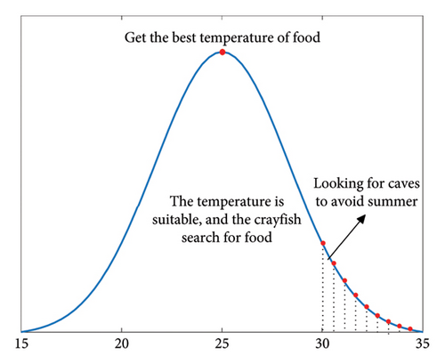
3.1.3. Summer Resort Phase
3.1.4. Competition Phase
3.1.5. Foraging Phase
The pseudocode for COA is outlined in Algorithm 1.
-
Algorithm 1: Crayfish optimization algorithm (COA).
-
Input: Maximum iteration number Tmax, population size N, dimension size D, current iteration t = 1
- 1.
Initialize the position of each crayfish using equation (2)
- 2.
Evaluate the fitness value of all crayfish individuals to gain ,
- 3.
Whilet ≤ Tmaxdo
- 4.
Calculate the current temperature value Temp using equation (3)
- 5.
Fordo
- 6.
IfTemp > 30then
- 7.
Calculate the location of the cave according to equation (5)
- 8.
Ifrand < 0.5then
- 9.
Update the current position of the crayfish using equation (6)
- 10.
Else
- 11.
Update the current position of the crayfish using equation (8)
- 12.
End If
- 13.
Else
- 14.
Define the food intake p and food size Q using equations (4) and (11), respectively
- 15.
If Q > (C3 + 1)/2then
- 16.
Update the current position of the crayfish using equation (13)
- 17.
Else
- 18.
Update the current position of the crayfish using equation (14)
- 19.
End If
- 20.
End If
- 21.
End For
- 22.
Calculate the fitness value of each individual
- 23.
Update ,
- 24.
t = t + 1
- 25.
End While
-
Return: Global optimal solution
3.2. Specular Reflection Learning
Opposition-based learning (OBL) serves as a robust search mechanism that concurrently evaluates the fitness values of the current solution alongside its opposite solution. This approach then filters out the superior candidate solution for inclusion in subsequent iterations [36]. Drawing inspiration from the concept of specular reflection, Zhang [37] introduced a specular reflection learning strategy by combining OBL with the specular reflection law. Unlike the one-to-one corresponding relationship between a solution and its opposite solution in OBL, specular reflection learning entails a correspondence between one solution and one neighborhood of its opposite solution.
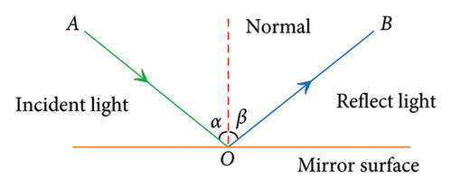
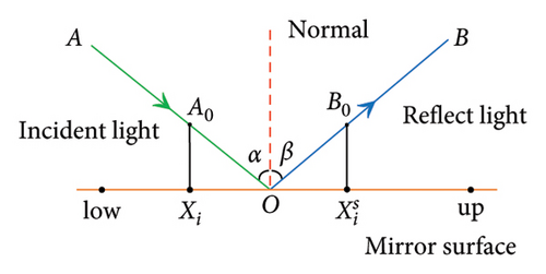
The initial positions of the population are generated using a randomized distribution mode. However, if the initial solution is distant from the global optimum or situated in the opposite direction, it may result in prolonged convergence time or even stagnation of the algorithm. In the early iterations, specular reflection learning facilitates a broader bidirectional simultaneous exploration of the solution space and increases the probability of finding the optimal solution.
3.3. Expanded Exploration Strategy
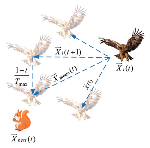
In COA, search agents in early iterations use equation (6) to conduct global exploration to identify areas where the global optimum may be present. This stage simulates the behavior of crayfish moving toward the cave for the summer resort, where the current position is updated based on and . However, due to the limited spatial information as well as insufficient population diversity, this approach cannot swiftly guide the algorithm into the correct search domain. Hence, the exploration capability of COA still needs to be strengthened. On the other hand, the exploration procedure of AO directly incorporates the global optimal position , allowing individuals to execute Aquila’s fast flight and predation maneuvers in the search space with faster convergence and better exploration competence. Considering the above, we hope to take advantage of the expanded exploration strategy (equation (20)) to replace the original position update formula (equation (6)), thus bringing a more stable exploration–exploitation balance and faster convergence speed to the algorithm.
3.4. Lévy Flight
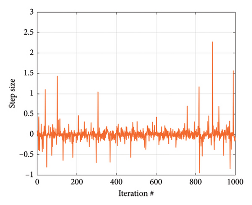
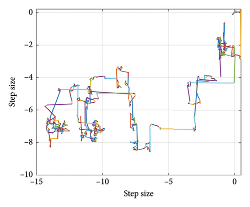
Lévy flight is a non-Gaussian stochastic walk method with step sizes taken from the Lévy probability distribution [39]. Figure 5 visualizes the distribution and 2D path of Lévy flight. Initially, the particle undergoes local movement, frequently taking numerous short-distance steps, and then occasionally embarks on a large step and commences a new cycle.
3.5. Vertical Crossover Operator
Here, F(·) indicates the fitness function. By using the vertical crossover strategy to perturb the position of the search agent, the algorithm’s local optima avoidance ability is enhanced, thereby further boosting convergence accuracy.
4. Proposed MCOA Algorithm
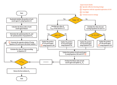
4.1. Detailed Implementation Steps for MCOA
- 1.
Specular reflection learning is introduced in the early iterations to enrich the population diversity and expand the search area.
- 2.
The expanded exploration strategy of AO is integrated with COA to replace its original position update formula, which endows the proposed method with better exploration capability and faster convergence speed.
- 3.
The Lévy flight step is embedded into the exploitation phase to improve the search efficiency in the neighborhood domain.
- 4.
The vertical crossover operator is applied in later iterations to randomly cross-perturb individual dimensions to further improve the solution accuracy.
-
Initialization
-
Step 1: Parameter setting: Maximum number of iterations Tmax, population size N, variable dimension D, and search range [LB, UB]. Fix the number of current iterations t = 1.
-
Step 2: Initialize the position of each search agent in the search space using equation (2).
-
Step 3: Evaluate the fitness value for each search agent Fitnessi(i = 1, 2, …, N) and record the optimal solution obtained so far and the optimal location for the whole population .
-
Iteration
-
Step 4: While t ≤ Tmax, perform specular reflection learning based on equation (19) to generate the corresponding opposite candidate solution for each individual and retain the superior one of both into the subsequent procedure.
-
Step 5: Calculate the ambient temperature value Temp using equation (3) to determine which position update strategy needs to be adopted in the following.
-
Step 6: If Temp > 30 and rand < 0.5, MCOA enters the exploration phase. The location of each search individual is updated using equation (20). Note that here and are equivalent, i.e., the current optimal solution.
-
Step 7: If Temp > 30 and rand ≥ 0.5, MCOA executes the competition exploitation strategy by updating the location of each search individual via equation (8).
-
Step 8: When Temp ≤ 30, MCOA performs the foraging exploitation strategy. Define the food intake p and food size Q using equations (4) and (11). In case Q > (C3 + 1)/2, update the location of each search individual using equations (12) and (13). Instead, update the location of each search individual using equation (22).
-
Step 9: Perform the vertical crossover operator to update the location of the population using equation (26).
-
Step 10: The fitness values of all search agents are reevaluated to update and .
-
Output
-
Step 11: Set t = t + 1; if t is greater than the maximum iteration termination criterion, output the global optimal solution ; otherwise, return to Step 4.
Figure 6 illustrates the flowchart of the proposed MCOA, while Algorithm 2 provides the pseudocode outlining the MCOA procedure.
-
Algorithm 2: Modified crayfish optimization algorithm with multistrategy (MCOA).
-
Input: Maximum iteration number Tmax, population size N, dimension size D, current iteration t = 1
- 1.
Initialize the position of each search agent using equation (2)
- 2.
Evaluate the fitness value of all search agents to gain ,
- 3.
Whilet ≤ Tmaxdo
- 4.
Perform the specular reflection learning to generate according to equation (19), and retain the better one of and into the next generation //Specular reflection learning
- 5.
Calculate the value of Temp using equation (3)
- 6.
Fordo
- 7.
IfTemp > 30then
- 8.
Calculate the value of using equation (5)
- 9.
Ifrand < 0.5then
- 10.
Update the current position of the search agent using equation (20) //Expanded exploration
- 11.
Else
- 12.
Update the current position of the search agent using equation (8)
- 13.
End If
- 14.
Else
- 15.
Define the food intake p and food size Q using equations (4) and (11), respectively
- 16.
IfQ > (C3 + 1)/2then
- 17.
Update the current position of the search agent using equation (13)
- 18.
Else
- 19.
Update the current position of the search agent using equation (22) //Lévy flight
- 20.
End If
- 21.
End If
- 22.
End For
- 23.
Perform the vertical crossover operator to update each search agent according to equations (26) and (27) //Vertical crossover strategy
- 24.
Evaluate the fitness value of all search agents
- 25.
Update ,
- 26.
t = t + 1
- 27.
End While
-
Return: Global optimal solution
4.2. Computational Complexity Analysis
The computational complexity of MCOA is determined by three main components: initialization, fitness evaluation, and position updating. The locations of all search individuals are randomly distributed in the search space during the initialization process with a computational complexity of O(N × D), where N is the population size and D is the problem dimension. In each iteration, the fitness values of all search agents’ positions are evaluated to obtain the current optimal solution as well as population optimal position , which needs to consume the computational complexity of O(N × Tmax), where Tmax is the maximum number of iterations. The computational complexity of updating the positions of all search individuals during the exploration and exploitation phases is O(N × D × Tmax). Moreover, the introduction of specular reflection learning and the vertical crossover operator to improve the optimization performance incurs an additional computational complexity of O(N × D × Tmax) + O(N × D × Tmax). Therefore, the total computational complexity of MCOA is: O(MCOA) = O(initialization) + O(fitness evaluation) + O(position update) = O(N × D) + O(N × Tmax) + O(3 × N × D × Tmax) = O(N × (D + Tmax + 3DTmax)).
5. Numerical Optimization Experiments
In this section, a set of numerical simulation studies are performed on the three IEEE CEC test suites: CEC 2005, CEC 2019, and CEC 2022 to thoroughly validate the effectiveness of MCOA. The implementation platform consists of hardware including an Intel(R) Core (TM) i7-13700F 2.10 GHz CPU with 32 GB RAM and MATLAB R2023b software running on Windows 10 operating system.
5.1. Benchmark Suites and Performance Indices
The CEC2005 suite comprises 23 classical functions [6] categorized as unimodal (F1∼F7, testing exploitation capability), multimodal (F8∼F13, assessing exploration and escape from local optima), and fixed-dimension multimodal (F14∼F23, evaluating stability). Functions F1∼F13 feature adjustable dimensions for testing scalability.
The CEC2019 test suite [42] contains 10 challenging functions designed for complex numerical optimization problems. In addition, this paper employs the popular CEC2022 test suite [43] to further demonstrate the superiority of MCOA. This test set includes not only unimodal (CEC2022-01) and multimodal functions (CEC2022-02∼CEC2022-05) but also hybrid functions (CEC2022-06∼CEC2022-08) as well as composition functions (CEC2022-09∼CEC2022-12). These functions are nonlinear, nonconvex, nonderivable, and closely resembling realistic optimization problems and can provide a comprehensive assessment of an algorithm’s tracking capability. Detailed descriptions of all benchmark functions appear in Tables A.1–A.5 (Appendix A Benchmark function description).
Performance evaluation employs two measures: mean fitness value (Mean) and standard deviation (Std), with statistical significance determined through the Wilcoxon rank-sum test [44] (significance level 0.05, where “+” indicates MCOA outperforms the comparison algorithm, “−” indicates underperformance, and “=” signifies no significant difference) and the Friedman ranking test [45] revealing each algorithm’s overall ranking (“Mean rank”) across all benchmarks.
5.2. Comparison With Different State-of-the-Art MH Algorithms on 23 Classical Functions
This subsection employs 12 advanced MH algorithms for comparison experiments with MCOA, namely, the original COA, AO [38], dandelion optimizer (DO) [46], snake optimizer (SO) [47], arithmetic optimization algorithm (AOA) [48], artificial rabbit optimization (ARO) [49], tunicate swarm algorithm (TSA) [50], slime mould algorithm (SMA) [51], wild horse optimizer (WHO) [52], liver cancer algorithm (LCA) [53], rime optimization algorithm (RIME) [54], and sand cat swarm optimization (SCSO) [55]. The maximum number of iterations Tmax and the population size N for each optimization method are fixed at 500 and 30, and other core parameters remain the same as those in the original literature, see Table 1. To avoid accidental errors as much as possible, all algorithms are implemented independently 30 times on each benchmark function.
| Algorithm | Year | Parameter value |
|---|---|---|
| AO | 2021 | ω = 0.005; R = 10; α = 0.1; δ = 0.1; g1 ∈ [−1, 1]; g2 = [2, 0] |
| DO | 2022 | α ∈ [0, 1]; k ∈ [0, 1] |
| SO | 2022 | c1 = 0.5; c2 = 0.05; c3 = 2 |
| AOA | 2021 | α = 5; μ = 0.499 |
| ARO | 2022 | — |
| TSA | 2020 | Pmin = 1; Pmax = 4 |
| SMA | 2020 | z = 0.03 |
| COA | 2023 | C1 = 0.2; C3 = 3; μ = 25; σ = 3 |
| WHO | 2021 | PC = 0.13; PS = 0.2; Crossover = Mean |
| LCA | 2023 | f = 1 |
| RIME | 2023 | w = 5 |
| SCSO | 2022 | rG = [2, 0]; SM = 2 |
5.2.1. Parameter Sensitivity Analysis
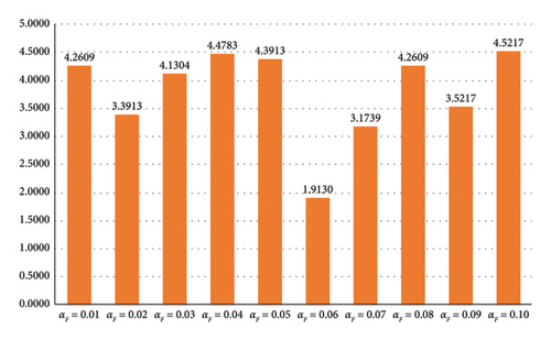
In Section 3.4, the addition of the Lévy flight strategy to the foraging phase of COA aims to enhance the search efficiency in locating potential food sources. The scale factor αF critically influences this improvement. If the value of αF is larger, the search agent will depend more on the optimal solution when updating its current position, and the algorithm is prone to premature convergence. Instead, a smaller αF value weakens the influence of Lévy flight on the guided foraging mechanism, leading to a decrease in the algorithm’s search capability and convergence accuracy. Based on the literature [32], the experimental range for αF is set between 0.01 and 0.1, with a value selected at each interval of 0.01. For each specified parameter value of αF, the results obtained by MCOA after 30 independent runs are shown in Table 2. With αF = 0.06, MCOA provides the most satisfactory solutions on 14 out of 23 test functions (60.87%), outperforming other values. For unimodal functions, MCOA performs consistently across different αF values on F1∼F4. The gap between the optimal solutions derived from different settings is also not particularly large on F5∼F7. The main reason is unimodal functions have fewer local solutions, which interfere less with the MCOA. For multimodal and fixed-dimension multimodal functions, a larger value of αF increases the step size of the Lévy operator, thus helping the proposed method to explore the search space more efficiently when facing complex optimization problems, especially on F8, F12, and F20. Figure 7 illustrates the Friedman mean rankings obtained by MCOA with different values of αF. MCOA exhibits the most desirable overall optimization performance when αF is 0.06, as it obtains the smallest ranking value of 1.9130. This indicates that this parameter value can balance exploration and exploitation favorably. Consequently, in the following sequence of experiments, taking αF = 0.06 is beneficial in avoiding local optimal solutions without affecting the sensitivity of the Lévy flight strategy and the algorithm’s convergence accuracy.
| Function | Metric | αF = 0.01 | αF = 0.02 | αF = 0.03 | αF = 0.04 | αF = 0.05 | αF = 0.06 | αF = 0.07 | αF = 0.08 | αF = 0.09 | αF = 0.1 |
|---|---|---|---|---|---|---|---|---|---|---|---|
| F1 | Mean | 0 | 0 | 0 | 0 | 0 | 0 | 0 | 0 | 0 | 0 |
| Std | 0 | 0 | 0 | 0 | 0 | 0 | 0 | 0 | 0 | 0 | |
| Rank | 1 | 1 | 1 | 1 | 1 | 1 | 1 | 1 | 1 | 1 | |
| F2 | Mean | 0 | 0 | 0 | 0 | 0 | 0 | 0 | 0 | 0 | 0 |
| Std | 0 | 0 | 0 | 0 | 0 | 0 | 0 | 0 | 0 | 0 | |
| Rank | 1 | 1 | 1 | 1 | 1 | 1 | 1 | 1 | 1 | 1 | |
| F3 | Mean | 0 | 0 | 0 | 0 | 0 | 0 | 0 | 0 | 0 | 0 |
| Std | 0 | 0 | 0 | 0 | 0 | 0 | 0 | 0 | 0 | 0 | |
| Rank | 1 | 1 | 1 | 1 | 1 | 1 | 1 | 1 | 1 | 1 | |
| F4 | Mean | 0 | 0 | 0 | 0 | 0 | 0 | 0 | 0 | 0 | 0 |
| Std | 0 | 0 | 0 | 0 | 0 | 0 | 0 | 0 | 0 | 0 | |
| Rank | 1 | 1 | 1 | 1 | 1 | 1 | 1 | 1 | 1 | 1 | |
| F5 | Mean | 1.2213E − 08 | 1.5859E − 06 | 9.3781E − 06 | 3.7685E − 06 | 2.5762E − 06 | 5.6298E − 08 | 1.2641E − 06 | 5.4132E − 06 | 8.3174E − 05 | 4.2134E − 05 |
| Std | 1.7049E − 08 | 2.1616E − 06 | 9.9527E − 06 | 3.8543E − 06 | 3.2459E − 06 | 7.9445E − 08 | 1.7644E − 06 | 6.0916E − 06 | 9.5472E − 05 | 5.6217E − 05 | |
| Rank | 1 | 4 | 8 | 6 | 5 | 2 | 3 | 7 | 10 | 9 | |
| F6 | Mean | 1.0933E − 21 | 1.5183E − 21 | 3.5111E − 21 | 1.5761E − 21 | 1.0039E − 19 | 3.3497E − 22 | 1.1515E − 19 | 5.4588E − 19 | 2.9277E − 22 | 3.0059E − 22 |
| Std | 4.7362E − 21 | 4.8629E − 21 | 1.6669E − 20 | 6.6035E − 21 | 4.6720E − 19 | 8.4095E − 22 | 5.7749E − 19 | 2.9868E − 18 | 6.2975E − 22 | 8.0293E − 22 | |
| Rank | 4 | 5 | 7 | 6 | 8 | 3 | 9 | 10 | 1 | 2 | |
| F7 | Mean | 3.7337E − 05 | 3.6381E − 05 | 4.4903E − 05 | 4.6794E − 05 | 5.0800E − 05 | 3.2531E − 05 | 2.9116E − 05 | 3.8652E − 05 | 4.0749E − 05 | 5.5205E − 05 |
| Std | 3.5815E − 05 | 4.1921E − 05 | 4.6964E − 05 | 4.2886E − 05 | 4.2928E − 05 | 2.7696E − 05 | 2.5914E − 05 | 2.6853E − 05 | 2.7816E − 05 | 7.1512E − 05 | |
| Rank | 4 | 3 | 7 | 8 | 9 | 2 | 1 | 5 | 6 | 10 | |
| F8 | Mean | −11772.32968 | −11761.48907 | −11787.84561 | −11812.18143 | −11742.52688 | −11853.70331 | −11784.61259 | −11803.85376 | −11739.794 | −11761.69685 |
| Std | 4.5979E + 02 | 3.2519E + 02 | 5.2271E + 02 | 3.9870E + 02 | 3.9325E + 02 | 3.0227E + 02 | 4.2833E + 02 | 4.8630E + 02 | 4.5192E + 02 | 3.1348E + 02 | |
| Rank | 6 | 8 | 4 | 2 | 9 | 1 | 5 | 3 | 10 | 7 | |
| F9 | Mean | 0 | 0 | 0 | 0 | 0 | 0 | 0 | 0 | 0 | 0 |
| Std | 0 | 0 | 0 | 0 | 0 | 0 | 0 | 0 | 0 | 0 | |
| Rank | 1 | 1 | 1 | 1 | 1 | 1 | 1 | 1 | 1 | 1 | |
| F10 | Mean | 8.8818E − 16 | 8.8818E − 16 | 8.8818E − 16 | 8.8818E − 16 | 8.8818E − 16 | 8.8818E − 16 | 8.8818E − 16 | 8.8818E − 16 | 8.8818E − 16 | 8.8818E − 16 |
| Std | 0 | 0 | 0 | 0 | 0 | 0 | 0 | 0 | 0 | 0 | |
| Rank | 1 | 1 | 1 | 1 | 1 | 1 | 1 | 1 | 1 | 1 | |
| F11 | Mean | 0 | 0 | 0 | 0 | 0 | 0 | 0 | 0 | 0 | 0 |
| Std | 0 | 0 | 0 | 0 | 0 | 0 | 0 | 0 | 0 | 0 | |
| Rank | 1 | 1 | 1 | 1 | 1 | 1 | 1 | 1 | 1 | 1 | |
| F12 | Mean | 1.6944E − 20 | 6.7606E − 22 | 4.8048E − 23 | 5.6620E − 22 | 4.1700E − 22 | 2.4595E − 23 | 1.7602E − 21 | 4.8386E − 22 | 3.7241E − 23 | 3.8594E − 22 |
| Std | 9.2709E − 20 | 2.7795E − 21 | 1.2321E − 22 | 2.3222E − 21 | 1.9451E − 21 | 1.0630E − 22 | 9.0052E − 21 | 2.0371E − 21 | 1.4032E − 22 | 1.8951E − 21 | |
| Rank | 10 | 8 | 3 | 7 | 5 | 1 | 9 | 6 | 2 | 4 | |
| F13 | Mean | 1.9120E − 21 | 4.8487E − 21 | 2.0410E − 17 | 2.5589E − 20 | 9.3884E − 22 | 2.3875E − 21 | 1.0154E − 21 | 1.9242E − 21 | 2.1038E − 20 | 1.0790E − 14 |
| Std | 8.5397E − 21 | 2.4178E − 20 | 1.1632E − 20 | 7.2840E − 20 | 2.4112E − 21 | 1.1178E − 16 | 3.2054E − 21 | 6.4821E − 21 | 8.2858E − 20 | 5.9102E − 14 | |
| Rank | 3 | 6 | 9 | 8 | 1 | 5 | 2 | 4 | 7 | 10 | |
| F14 | Mean | 1.3917E + 00 | 9.9800E − 01 | 1.3871E + 00 | 1.3917E + 00 | 1.5885E + 00 | 1.3917E + 00 | 1.1948E + 00 | 1.3917E + 00 | 9.9800E − 01 | 1.1948E + 00 |
| Std | 1.4982E + 00 | 0 | 2.1311E + 00 | 1.4982E + 00 | 1.8019E + 00 | 1.4982E + 00 | 1.0782E + 00 | 1.4982E + 00 | 0 | 1.0782E + 00 | |
| Rank | 9 | 1 | 5 | 8 | 10 | 5 | 3 | 5 | 1 | 3 | |
| F15 | Mean | 3.1278E − 04 | 3.1264E − 04 | 3.1472E − 04 | 3.1509E − 04 | 3.2881E − 04 | 3.0982E − 04 | 3.1116E − 04 | 3.1855E − 04 | 3.1267E − 04 | 3.8859E − 04 |
| Std | 1.5063E − 05 | 9.8728E − 06 | 1.2612E − 05 | 1.5755E − 05 | 9.7831E − 05 | 6.4028E − 06 | 8.5334E − 06 | 2.4872E − 05 | 1.4389E − 05 | 2.3911E − 04 | |
| Rank | 5 | 3 | 6 | 7 | 9 | 1 | 2 | 8 | 4 | 10 | |
| F16 | Mean | −1.0316 | −1.0316 | −1.0316 | −1.0316 | −1.0316 | −1.0316 | −1.0316 | −1.0316 | −1.0316 | −1.0316 |
| Std | 1.1005E − 10 | 5.7139E − 11 | 2.5934E − 11 | 4.2697E − 11 | 3.2594E − 11 | 4.5518E − 11 | 8.4454E − 11 | 5.5814E − 11 | 6.9643E − 11 | 7.5303E − 11 | |
| Rank | 10 | 6 | 1 | 3 | 2 | 4 | 9 | 5 | 7 | 8 | |
| F17 | Mean | 0.3979 | 0.3979 | 0.3979 | 0.3979 | 0.3979 | 0.3979 | 0.3979 | 0.3979 | 0.3979 | 0.3979 |
| Std | 1.5403E − 05 | 3.7291E − 06 | 8.0940E − 06 | 9.6520E − 06 | 8.8392E − 06 | 4.8362E − 06 | 2.1947E − 06 | 2.4870E − 05 | 7.9734E − 06 | 7.0392E − 06 | |
| Rank | 9 | 2 | 6 | 8 | 7 | 3 | 1 | 10 | 5 | 4 | |
| F18 | Mean | 3.0000 | 3.9000 | 3.0000 | 3.9000 | 3.0000 | 3.0000 | 3.0000 | 3.9000 | 3.0000 | 3.0000 |
| Std | 9.2199E − 16 | 4.9295E + 00 | 9.9643E − 16 | 4.9295E + 00 | 1.0464E − 15 | 1.1337E − 16 | 1.1095E − 15 | 4.9295E + 00 | 1.0784E − 15 | 1.2506E − 15 | |
| Rank | 2 | 8 | 3 | 8 | 4 | 1 | 6 | 8 | 5 | 7 | |
| F19 | Mean | −3.8628 | −3.8628 | −3.8628 | −3.8628 | −3.8628 | −3.8628 | −3.8628 | −3.8628 | −3.8628 | −3.8628 |
| Std | 2.7101E − 15 | 2.7101E − 15 | 2.7101E − 15 | 2.7101E − 15 | 2.7101E − 15 | 2.7101E − 15 | 2.7101E − 15 | 2.7101E − 15 | 2.7101E − 15 | 2.7101E − 15 | |
| Rank | 1 | 1 | 1 | 1 | 1 | 1 | 1 | 1 | 1 | 1 | |
| F20 | Mean | −3.3101 | −3.3061 | −3.2982 | −3.3101 | −3.3022 | −3.3220 | −3.3141 | −3.3180 | −3.3022 | −3.3220 |
| Std | 3.6278E − 02 | 4.1107E − 02 | 4.8370E − 02 | 3.6278E − 02 | 4.5066E − 02 | 7.5540E − 13 | 3.0164E − 02 | 2.1707E − 02 | 4.5066E − 02 | 2.5036E − 11 | |
| Rank | 5 | 7 | 10 | 6 | 9 | 1 | 4 | 3 | 8 | 2 | |
| F21 | Mean | −10.1532 | −10.1532 | −10.1532 | −10.1532 | −10.1532 | −10.1532 | −10.1532 | −10.1532 | −10.1532 | −10.1532 |
| Std | 7.1207E − 15 | 7.2269E − 15 | 7.1740E − 15 | 7.2269E − 15 | 7.1740E − 15 | 7.1207E − 15 | 7.1740E − 15 | 7.2269E − 15 | 7.0670E − 15 | 7.2269E − 15 | |
| Rank | 2 | 7 | 4 | 7 | 4 | 2 | 4 | 7 | 1 | 7 | |
| F22 | Mean | −10.4029 | −10.4029 | −10.4029 | −10.4029 | −10.4029 | −10.4029 | −10.4029 | −10.4029 | −10.4029 | −10.4029 |
| Std | 1.8915E − 10 | 9.3299E − 16 | 1.0940E − 15 | 1.1893E − 15 | 1.1893E − 15 | 1.0431E − 15 | 9.8958E − 16 | 9.3299E − 16 | 1.0940E − 15 | 2.4629E − 11 | |
| Rank | 10 | 1 | 5 | 7 | 7 | 4 | 3 | 1 | 5 | 9 | |
| F23 | Mean | −10.5364 | −10.5364 | −10.5364 | −10.5364 | −10.5364 | −10.5364 | −10.5364 | −10.5364 | −10.5364 | −10.5364 |
| Std | 3.9729E − 09 | 1.8067E − 15 | 1.9792E − 15 | 1.8949E − 15 | 1.8949E − 15 | 1.8067E − 15 | 1.8949E − 15 | 1.9515E − 15 | 1.8067E − 15 | 1.8949E − 15 | |
| Rank | 10 | 1 | 9 | 4 | 4 | 1 | 4 | 8 | 1 | 4 | |
- Note: The best results obtained are highlighted in bold.
5.2.2. Qualitative Analysis
This subsection presents a qualitative analysis to visualize the optimization dynamics of the proposed algorithm throughout the iterative process. Four unimodal, four multimodal, and two fixed-dimension multimodal benchmark functions are selected for testing. As shown in Figure 8, the first column depicts the topological structure of each function in two-dimensional space. The second to sixth columns, respectively, display: (1) convergence curves, (2) search trajectories in the first dimension, (3) average fitness values, (4) search history of the first two agents, and (5) trends in exploration and exploitation percentages.
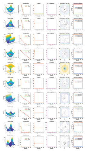
The convergence curves demonstrate how each algorithm progresses toward the optimal solution. Compared to COA, MCOA converges faster and achieves the desired convergence accuracy with fewer iterations in most test cases. On F1 and F3, both COA and MCOA converge to the global optimal point (0), but the latter requires fewer iterations. On F5 and F6, MCOA demonstrates stronger exploitation capabilities and achieves much higher convergence accuracy, thanks to its enhanced search mechanism guided by the Lévy flight strategy. For multimodal and fixed-dimension multimodal functions, both algorithms exhibit similar convergence accuracy and speed on F10, F11, and F18. However, on F12, F13, and F15, MCOA clearly has better local optimal avoidance, and the curve gradually decreases toward the global optimal solution.
The iteration trajectory can be approximated from the third column in Figure 8. In the early stages of iterations, the curves show large oscillations, indicating that the algorithm favors exploration at this stage. In the medium and late iterations, the curves gradually flatten out, which implies that exploitation is utilized to ensure that MCOA converges to a higher level of accuracy.
The average fitness value represents the average target optimal value of all dimensions in each iteration and is used to characterize the evolutionary tendency of the whole population. All the curves exhibit a significant decrease over iterations, suggesting that MCOA can quickly steer the population closer to the global optimum.
The search history illustrates the locations where the search agent has explored in its quest to find the global optimum during the optimization process. The red dot marks the best solution found within the given iteration limit. Many search agents are centered around the optimal solution, suggesting that MCOA is more inclined to exploit promising solutions. Additionally, the dispersion and traversal of search agents across the search space validate the excellent search breadth of MCOA.
Finally, the last column shows how MCOA balances exploration and exploitation based on a dimension-wise diversity model [56]. In the initial iteration stage, MCOA exhibits a high level of exploration to thoroughly explore the search space and locate promising regions. As iterations progress, the percentage of exploitation gradually increases, ensuring accuracy of the final solution. Throughout this procedure, MCOA achieves a smooth transition from exploration to exploitation. This figure also captures the switching time points between these two key components for MCOA.
5.2.3. Ablation Analysis of Multiple Improvement Strategies
In this subsection, an ablation analysis experiment is designed to verify the effectiveness of each improvement strategy. Table 3 outlines the 10 derivative variants of MCOA, where 1 indicates activation of the corresponding strategy, while 0 indicates its absence. COA, MCOA, and other different MCOA derivatives are tested simultaneously on 23 benchmark problems, and the results are shown in Table 4.
| Strategy | MCOA-1 | MCOA-2 | MCOA-3 | MCOA-4 | MCOA-5 | MCOA-6 | MCOA-7 | MCOA-8 | MCOA-9 | MCOA-10 | MCOA |
|---|---|---|---|---|---|---|---|---|---|---|---|
| Specular reflection learning | 1 | 0 | 0 | 0 | 1 | 1 | 1 | 0 | 0 | 0 | 1 |
| Expanded exploration | 0 | 1 | 0 | 0 | 1 | 0 | 0 | 1 | 1 | 0 | 1 |
| Lévy flight | 0 | 0 | 1 | 0 | 0 | 1 | 0 | 1 | 0 | 1 | 1 |
| Vertical crossover operator | 0 | 0 | 0 | 1 | 0 | 0 | 1 | 0 | 1 | 1 | 1 |
| Function | Metric | COA | MCOA-1 | MCOA-2 | MCOA-3 | MCOA-4 | MCOA-5 | MCOA-6 | MCOA-7 | MCOA-8 | MCOA-9 | MCOA-10 | MCOA |
|---|---|---|---|---|---|---|---|---|---|---|---|---|---|
| F1 | Mean | 0 | 0 | 0 | 0 | 0 | 0 | 0 | 0 | 0 | 0 | 0 | 0 |
| Std | 0 | 0 | 0 | 0 | 0 | 0 | 0 | 0 | 0 | 0 | 0 | 0 | |
| Rank | 1 | 1 | 1 | 1 | 1 | 1 | 1 | 1 | 1 | 1 | 1 | 1 | |
| F2 | Mean | 0 | 0 | 0 | 0 | 0 | 0 | 0 | 0 | 0 | 0 | 0 | 0 |
| Std | 0 | 0 | 0 | 0 | 0 | 0 | 0 | 0 | 0 | 0 | 0 | 0 | |
| Rank | 1 | 1 | 1 | 1 | 1 | 1 | 1 | 1 | 1 | 1 | 1 | 1 | |
| F3 | Mean | 0 | 0 | 0 | 0 | 0 | 0 | 0 | 0 | 0 | 0 | 0 | 0 |
| Std | 0 | 0 | 0 | 0 | 0 | 0 | 0 | 0 | 0 | 0 | 0 | 0 | |
| Rank | 1 | 1 | 1 | 1 | 1 | 1 | 1 | 1 | 1 | 1 | 1 | 1 | |
| F4 | Mean | 0 | 0 | 0 | 0 | 0 | 0 | 0 | 0 | 0 | 0 | 0 | 0 |
| Std | 0 | 0 | 0 | 0 | 0 | 0 | 0 | 0 | 0 | 0 | 0 | 0 | |
| Rank | 1 | 1 | 1 | 1 | 1 | 1 | 1 | 1 | 1 | 1 | 1 | 1 | |
| F5 | Mean | 2.8339E + 00 | 2.8229E + 00 | 9.4824E − 01 | 2.6837E + 00 | 2.5733E + 00 | 1.6028E − 03 | 2.6606E + 00 | 2.8015E + 00 | 1.8943E + 00 | 1.2088E − 03 | 2.6158E + 00 | 6.5468E − 10 |
| Std | 8.6474E + 00 | 8.6137E + 00 | 5.1048E + 00 | 8.1899E + 00 | 7.8531E + 00 | 8.0295E − 03 | 8.1201E + 00 | 8.5493E + 00 | 7.1088E + 00 | 5.4444E − 03 | 7.9825E + 00 | 3.3974E − 09 | |
| Rank | 12 | 11 | 4 | 9 | 6 | 3 | 8 | 10 | 5 | 2 | 7 | 1 | |
| F6 | Mean | 4.9581E − 01 | 3.6394E − 01 | 9.2552E − 04 | 4.6614E − 01 | 4.4874E − 08 | 2.7375E − 05 | 3.9998E − 01 | 2.9657E − 18 | 5.8338E − 04 | 3.0936E − 08 | 3.6069E − 08 | 1.1042E − 21 |
| Std | 3.5948E − 01 | 2.7476E − 01 | 1.8400E − 03 | 2.8322E − 01 | 5.9490E − 08 | 2.2632E − 05 | 2.7702E − 01 | 1.5185E − 17 | 9.9238E − 04 | 4.9425E − 08 | 2.8818E − 08 | 5.3596E − 21 | |
| Rank | 12 | 9 | 8 | 11 | 5 | 6 | 10 | 2 | 7 | 3 | 4 | 1 | |
| F7 | Mean | 8.1905E − 05 | 1.1367E − 04 | 6.3096E − 05 | 6.8164E − 05 | 4.1200E − 05 | 5.3659E − 05 | 7.8830E − 05 | 3.6702E − 05 | 7.9099E − 05 | 4.4214E − 05 | 3.6104E − 05 | 3.5231E − 05 |
| Std | 8.4466E − 05 | 1.0435E − 04 | 5.8071E − 05 | 6.8581E − 05 | 4.3879E − 05 | 4.6726E − 05 | 7.1452E − 05 | 3.2258E − 05 | 1.1355E − 04 | 3.5477E − 05 | 3.4912E − 05 | 3.0745E − 05 | |
| Rank | 11 | 12 | 7 | 8 | 4 | 6 | 9 | 3 | 10 | 5 | 2 | 1 | |
| F8 | Mean | −5242.7189 | −8686.5444 | −8329.8712 | −8106.5679 | −11587.9782 | −8213.3889 | −8658.6230 | −11691.5067 | −5573.7303 | −11508.0893 | −11714.0076 | −11829.1962 |
| Std | 6.8306E + 02 | 6.7034E + 02 | 1.3453E + 03 | 1.3844E + 03 | 4.8453E + 02 | 2.8154E + 03 | 6.9393E + 02 | 3.9648E + 02 | 1.5700E + 03 | 5.0753E + 02 | 4.0317E + 02 | 3.8003E + 02 | |
| Rank | 12 | 6 | 8 | 10 | 4 | 9 | 7 | 3 | 11 | 5 | 2 | 1 | |
| F9 | Mean | 0 | 0 | 0 | 0 | 0 | 0 | 0 | 0 | 0 | 0 | 0 | 0 |
| Std | 0 | 0 | 0 | 0 | 0 | 0 | 0 | 0 | 0 | 0 | 0 | 0 | |
| Rank | 1 | 1 | 1 | 1 | 1 | 1 | 1 | 1 | 1 | 1 | 1 | 1 | |
| F10 | Mean | 8.8818E − 16 | 8.8818E − 16 | 8.8818E − 16 | 8.8818E − 16 | 8.8818E − 16 | 8.8818E − 16 | 8.8818E − 16 | 8.8818E − 16 | 8.8818E − 16 | 8.8818E − 16 | 8.8818E − 16 | 8.8818E − 16 |
| Std | 0 | 0 | 0 | 0 | 0 | 0 | 0 | 0 | 0 | 0 | 0 | 0 | |
| Rank | 1 | 1 | 1 | 1 | 1 | 1 | 1 | 1 | 1 | 1 | 1 | 1 | |
| F11 | Mean | 0 | 0 | 0 | 0 | 0 | 0 | 0 | 0 | 0 | 0 | 0 | 0 |
| Std | 0 | 0 | 0 | 0 | 0 | 0 | 0 | 0 | 0 | 0 | 0 | 0 | |
| Rank | 1 | 1 | 1 | 1 | 1 | 1 | 1 | 1 | 1 | 1 | 1 | 1 | |
| F12 | Mean | 1.4950E − 02 | 1.3070E − 02 | 4.9624E − 05 | 1.4443E − 02 | 1.9757E − 09 | 2.1801E − 06 | 1.2297E − 02 | 8.1146E − 21 | 5.8363E − 05 | 1.3261E − 09 | 1.7528E − 09 | 4.4560E − 22 |
| Std | 1.3620E − 02 | 7.5554E − 03 | 1.2902E − 04 | 1.1037E − 02 | 2.1721E − 09 | 2.3345E − 06 | 9.2124E − 03 | 3.1105E − 20 | 8.9406E − 05 | 2.3415E − 09 | 2.0703E − 09 | 1.5576E − 21 | |
| Rank | 12 | 10 | 7 | 11 | 5 | 6 | 9 | 2 | 8 | 3 | 4 | 1 | |
| F13 | Mean | 2.5461E + 00 | 2.6629E + 00 | 1.1824E − 03 | 2.2444E + 00 | 9.8869E − 02 | 1.8785E + 00 | 2.1944E + 00 | 2.8123E − 07 | 3.0870E − 03 | 8.0494E − 09 | 3.7913E − 05 | 1.4575E − 21 |
| Std | 6.9273E − 01 | 6.5553E − 01 | 2.0458E − 03 | 2.8428E − 01 | 5.4153E − 01 | 1.4538E + 00 | 2.4985E − 01 | 4.0820E − 07 | 1.4676E − 02 | 1.5178E − 08 | 3.4548E − 05 | 6.1017E − 21 | |
| Rank | 11 | 12 | 5 | 10 | 7 | 8 | 9 | 3 | 6 | 2 | 4 | 1 | |
| F14 | Mean | 5.4081E + 00 | 2.6649E + 00 | 2.8500E + 00 | 3.4750E + 00 | 9.9800E − 01 | 2.7697E + 00 | 2.8928E + 00 | 1.1948E + 00 | 3.6212E + 00 | 2.1653E + 00 | 1.6159E + 00 | 9.9800E − 01 |
| Std | 4.9117E + 00 | 3.2382E + 00 | 3.4574E + 00 | 4.1251E + 00 | 1.7001E − 16 | 2.7369E + 00 | 3.4534E + 00 | 1.0782E + 00 | 4.0354E + 00 | 3.5616E + 00 | 2.4347E + 00 | 0 | |
| Rank | 12 | 6 | 8 | 10 | 2 | 7 | 9 | 3 | 11 | 5 | 4 | 1 | |
| F15 | Mean | 3.2644E − 03 | 4.4858E − 04 | 3.9398E − 04 | 1.2984E − 03 | 4.7506E − 04 | 3.9651E − 04 | 4.2208E − 04 | 3.3332E − 04 | 4.3627E − 04 | 3.1380E − 04 | 4.7124E − 04 | 3.1322E − 04 |
| Std | 6.8257E − 03 | 1.9829E − 04 | 1.9152E − 04 | 3.6113E − 03 | 2.4168E − 04 | 2.5464E − 04 | 1.3001E − 04 | 5.3566E − 05 | 2.9654E − 04 | 1.7453E − 05 | 2.0537E − 04 | 8.6955E − 06 | |
| Rank | 12 | 8 | 4 | 11 | 10 | 5 | 6 | 3 | 7 | 2 | 9 | 1 | |
| F16 | Mean | −1.0316 | −1.0316 | −1.0316 | −1.0316 | −1.0316 | −1.0316 | −1.0316 | −1.0316 | −1.0316 | −1.0316 | −1.0316 | −1.0316 |
| Std | 1.3592E − 10 | 9.7968E − 12 | 8.7392E − 12 | 7.4590E − 15 | 7.8949E − 12 | 2.4479E − 11 | 1.6049E − 15 | 9.4566E − 16 | 1.6421E − 15 | 2.1587E − 15 | 7.6919E − 16 | 6.2532E − 16 | |
| Rank | 12 | 10 | 9 | 7 | 8 | 11 | 4 | 3 | 5 | 6 | 2 | 1 | |
| F17 | Mean | 0.3979 | 0.3979 | 0.3979 | 0.3979 | 0.3979 | 0.3979 | 0.3979 | 0.3979 | 0.3979 | 0.3979 | 0.3979 | 0.3979 |
| Std | 1.2830E − 05 | 8.3105E − 06 | 3.1170E − 06 | 4.1011E − 05 | 9.7162E − 09 | 6.6459E − 09 | 5.3952E − 08 | 7.1487E − 08 | 1.1628E − 05 | 1.1803E − 09 | 3.1557E − 09 | 1.4768E − 09 | |
| Rank | 11 | 9 | 8 | 12 | 5 | 4 | 6 | 7 | 10 | 1 | 3 | 2 | |
| F18 | Mean | 3.9000 | 3.0000 | 3.0000 | 3.0000 | 3.0000 | 3.0000 | 3.0000 | 3.0000 | 3.0000 | 3.0000 | 3.0000 | 3.0000 |
| Std | 4.9295E + 00 | 5.0484E − 06 | 1.9001E − 05 | 5.6397E − 11 | 2.4269E − 11 | 1.2397E − 15 | 1.2259E − 15 | 2.9733E − 16 | 4.9479E − 16 | 9.3201E − 12 | 1.0464E − 11 | 5.0835E − 16 | |
| Rank | 12 | 10 | 11 | 9 | 8 | 5 | 4 | 1 | 2 | 6 | 7 | 3 | |
| F19 | Mean | −3.8625 | −3.8628 | −3.8628 | −3.8370 | −3.8628 | −3.8628 | −3.8628 | −3.8628 | −3.8628 | −3.8628 | −3.8628 | −3.8628 |
| Std | 1.4390E − 03 | 1.1418E − 12 | 5.0657E − 09 | 1.4113E − 01 | 6.0842E − 13 | 2.7101E − 15 | 2.7101E − 15 | 2.7101E − 15 | 9.4576E − 09 | 3.8424E − 09 | 2.7101E − 15 | 2.7101E − 15 | |
| Rank | 11 | 7 | 9 | 12 | 6 | 1 | 1 | 1 | 10 | 8 | 1 | 1 | |
| F20 | Mean | −3.2565 | −3.2903 | −3.2900 | −3.2785 | −3.2774 | −3.2863 | −3.2943 | −3.3101 | −3.3180 | −3.2982 | −3.3220 | −3.3220 |
| Std | 7.7179E − 02 | 5.3481E − 02 | 5.3297E − 02 | 6.5862E − 02 | 5.7641E − 02 | 5.5415E − 02 | 5.1147E − 02 | 3.6278E − 02 | 2.1707E − 02 | 4.8370E − 02 | 4.1485E − 09 | 4.4621E − 09 | |
| Rank | 12 | 7 | 8 | 10 | 11 | 9 | 6 | 4 | 3 | 5 | 1 | 2 | |
| F21 | Mean | −7.2776 | −9.4735 | −8.7936 | −7.4343 | −9.1336 | −8.6237 | −9.9833 | −10.1532 | −10.1532 | −9.4735 | −9.8133 | −10.1532 |
| Std | 2.7974E + 00 | 1.7626E + 00 | 2.2929E + 00 | 2.5868E + 00 | 2.0741E + 00 | 2.3761E + 00 | 9.3076E − 01 | 6.8855E − 12 | 7.2269E − 15 | 1.7626E + 00 | 1.2934E + 00 | 7.1207E − 15 | |
| Rank | 12 | 7 | 9 | 11 | 8 | 10 | 4 | 3 | 2 | 6 | 5 | 1 | |
| F22 | Mean | −7.1337 | −9.4176 | −10.0485 | −7.4907 | −10.2258 | −9.8714 | −9.6826 | −10.4029 | −10.4029 | −10.4029 | −10.0500 | −10.4029 |
| Std | 3.2066E + 00 | 2.0430E + 00 | 1.3485E + 00 | 2.8020E + 00 | 9.7043E − 01 | 1.6218E + 00 | 1.8342E + 00 | 4.4101E − 09 | 7.4927E − 05 | 9.3299E − 16 | 1.3433E + 00 | 3.2986E − 16 | |
| Rank | 12 | 10 | 7 | 11 | 5 | 8 | 9 | 3 | 4 | 2 | 6 | 1 | |
| F23 | Mean | −7.5558 | −10.3561 | −10.1758 | −7.7540 | −10.5364 | −10.5364 | −10.5364 | −10.5364 | −10.3561 | −10.5364 | −10.5364 | −10.5364 |
| Std | 3.1046E + 00 | 9.8735E − 01 | 1.3720E + 00 | 3.1145E + 00 | 1.6546E − 09 | 2.0600E − 15 | 1.5055E − 08 | 8.8723E − 10 | 9.8734E − 01 | 5.9927E − 08 | 3.4279E − 09 | 1.8949E − 15 | |
| Rank | 12 | 8 | 10 | 11 | 4 | 2 | 6 | 3 | 9 | 7 | 5 | 1 | |
| Mean rank | 8.4783 | 6.4783 | 5.6087 | 7.3913 | 4.5652 | 4.6522 | 4.9565 | 2.6522 | 5.0870 | 3.2609 | 3.1739 | 1.1739 | |
| Final ranking | 12 | 10 | 9 | 11 | 5 | 6 | 7 | 2 | 8 | 4 | 3 | 1 | |
- Note: The best results obtained are highlighted in bold.
As shown in Table 4, MCOA achieves the best overall performance with a Friedman mean ranking of 1.1739, significantly outperforming all variant algorithms and the original COA. When examining individual strategies, their effectiveness can be quantitatively ranked from highest to lowest impact: vertical crossover operator (MCOA-4, rank 5.5652), expanded exploration strategy (MCOA-2, rank 5.6087), specular reflection learning (MCOA-1, rank 6.4783), and Lévy flight (MCOA-3, rank 7.3913).
The vertical crossover operator demonstrates exceptional local exploitation capability, evidenced by MCOA-9’s superior performance on unimodal functions F5, F6, and F7, where precise local search is critical. For multimodal functions, the expanded exploration strategy (MCOA-2) yields the best results among single-strategy variants, showing significantly lower mean values compared to COA, particularly on functions F8 (−8329.8712 vs. −5242.7189) and F13(1.1824E-03 vs. 2.5461E + 00). This confirms its effectiveness in overcoming COA’s exploration deficiencies while preserving exploitation strength.
Furthermore, the synergistic integration of these strategies in MCOA produces remarkably consistent performance, achieving optimal results on 18 of 23 benchmark functions with minimal standard deviations, particularly on complex multimodal functions. For instance, on F8, the mean value of MCOA is −11829.1962, while the mean value of COA is −5242.7189, representing a 125.6% improvement. The combination of specular reflection learning and vertical crossover operator (MCOA-7) proves particularly effective for navigating local optima traps, as evidenced by its second-place overall ranking (2.6522), demonstrating how complementary strategies enhance both exploration and exploitation phases. Specular reflection learning and expanded exploration strategy enhance exploration, whereas Lévy flight and vertical crossover operator focus on strengthening exploitation, synergistically leading MCOA toward the optimal solution.
5.2.4. Quantitative Analysis
In this subsection, we quantitatively evaluate the numerical optimization performance of MCOA against twelve established MH algorithms: AO, DO, SO, AOA, ARO, TSA, SMA, COA, WHO, LCA, RIME, and SCSO. The statistical results are presented in Table 5.
| Function | Metric | MCOA | AO | DO | SO | AOA | ARO | TSA | SMA | COA | WHO | LCA | RIME | SCSO |
|---|---|---|---|---|---|---|---|---|---|---|---|---|---|---|
| F1 | Mean | 0 | 1.2014E − 101 | 1.1698E − 05 | 1.4548E − 94 | 3.9390E − 35 | 3.8009E − 65 | 6.6645E − 195 | 0 | 0 | 2.2857E − 44 | 2.0725E − 01 | 1.9599E + 00 | 2.1307E − 110 |
| Std | 0 | 6.5804E − 101 | 6.4523E − 06 | 3.4672E − 94 | 2.1575E − 34 | 2.0495E − 64 | 0 | 0 | 0 | 6.4927E − 44 | 2.4941E − 01 | 8.2185E − 01 | 1.1671E − 109 | |
| p value | — | 1.2118E − 12 | 1.2118E − 12 | 1.2118E − 12 | 1.2118E − 12 | 1.2118E − 12 | 1.2118E − 12 | NaN | NaN | 1.2118E − 12 | 1.2118E − 12 | 1.2118E − 12 | 1.2118E − 12 | |
| Rank | 1 | 6 | 11 | 7 | 10 | 8 | 4 | 1 | 1 | 9 | 12 | 13 | 5 | |
| F2 | Mean | 0 | 1.2580E − 52 | 1.5150E − 03 | 5.1539E − 43 | 0 | 5.5376E − 36 | 4.3975E − 100 | 0 | 0 | 9.4366E − 24 | 1.7163E − 01 | 1.7947E + 00 | 4.9236E − 61 |
| Std | 0 | 6.8904E − 52 | 7.7126E − 04 | 1.2954E − 42 | 0 | 1.2643E − 35 | 1.9856E − 99 | 0 | 0 | 5.0227E − 23 | 1.9407E − 01 | 1.4158E + 00 | 9.4981E − 61 | |
| p value | — | 1.2118E − 12 | 1.2118E − 12 | 1.2118E − 12 | NaN | 1.2118E − 12 | 1.2118E − 12 | NaN | NaN | 1.2118E − 12 | 1.2118E − 12 | 1.2118E − 12 | 1.2118E − 12 | |
| Rank | 1 | 7 | 11 | 8 | 1 | 9 | 5 | 1 | 1 | 10 | 12 | 13 | 6 | |
| F3 | Mean | 0 | 2.7322E − 99 | 2.4004E + 01 | 2.7757E − 56 | 1.0008E − 02 | 5.9800E − 49 | 2.9285E − 182 | 0 | 0 | 1.9650E − 21 | 3.8052E + 01 | 1.3895E + 03 | 5.6172E − 111 |
| Std | 0 | 1.4965E − 98 | 1.8300E + 01 | 1.5105E − 55 | 1.5955E − 02 | 3.2090E − 48 | 0 | 0 | 0 | 1.0762E − 20 | 3.8905E + 01 | 4.0077E + 02 | 2.6073E − 110 | |
| p value | — | 1.2118E − 12 | 1.2118E − 12 | 1.2118E − 12 | 1.2118E − 12 | 1.2118E − 12 | 1.2118E − 12 | NaN | NaN | 1.2118E − 12 | 1.2118E − 12 | 1.2118E − 12 | 1.2118E − 12 | |
| Rank | 1 | 6 | 11 | 7 | 10 | 8 | 4 | 1 | 1 | 9 | 12 | 13 | 5 | |
| F4 | Mean | 0 | 1.0076E − 53 | 9.2019E − 01 | 9.8256E − 41 | 2.6076E − 02 | 3.6544E − 27 | 1.1759E − 91 | 0 | 0 | 2.6781E − 16 | 8.3346E − 02 | 7.1134E + 00 | 6.0476E − 59 |
| Std | 0 | 5.5085E − 53 | 6.8201E − 01 | 1.6184E − 40 | 2.0631E − 02 | 1.6360E − 26 | 3.7854E − 91 | 0 | 0 | 1.3583E − 15 | 5.5805E − 02 | 2.5478E + 00 | 2.1111E − 58 | |
| p value | — | 1.2118E − 12 | 1.2118E − 12 | 1.2118E − 12 | 1.2118E − 12 | 1.2118E − 12 | 1.2118E − 12 | NaN | NaN | 1.2118E − 12 | 1.2118E − 12 | 1.2118E − 12 | 1.2118E − 12 | |
| Rank | 1 | 6 | 12 | 7 | 10 | 8 | 4 | 1 | 1 | 9 | 11 | 13 | 5 | |
| F5 | Mean | 1.5982E − 07 | 8.0245E − 04 | 1.2713E + 01 | 8.1014E + 00 | 9.5104E + 00 | 1.1935E + 00 | 9.5724E + 00 | 3.7068E + 00 | 8.9767E + 00 | 1.2470E + 01 | 5.5234E − 01 | 1.1965E + 02 | 9.6259E + 00 |
| Std | 5.4520E − 07 | 1.7527E − 03 | 2.0941E + 01 | 1.2851E + 01 | 1.3642E + 01 | 4.9565E + 00 | 1.3770E + 01 | 9.2134E + 00 | 1.2927E + 01 | 2.1930E + 01 | 1.7195E + 00 | 3.1563E + 02 | 1.3846E + 01 | |
| p value | — | 1.7072E − 04 | 1.2710E − 11 | 1.7072E − 04 | 1.6025E − 09 | 1.7072E − 04 | 1.7072E − 04 | 3.8303E − 03 | 3.8303E − 03 | 1.7072E − 04 | 1.2710E − 11 | 1.2710E − 11 | 1.7072E − 04 | |
| Rank | 1 | 2 | 12 | 6 | 8 | 4 | 9 | 5 | 7 | 11 | 3 | 13 | 10 | |
| F6 | Mean | 1.1124E − 22 | 1.1238E − 04 | 1.7637E − 05 | 1.0880E + 00 | 3.1760E + 00 | 4.3183E − 03 | 6.1029E + 00 | 3.3753E − 03 | 3.4253E − 01 | 1.4773E − 02 | 1.9287E − 01 | 2.4266E + 00 | 2.5319E + 00 |
| Std | 2.1677E − 22 | 3.3118E − 04 | 7.9050E − 06 | 8.8946E − 01 | 2.3486E − 01 | 2.0796E − 03 | 9.6084E − 01 | 1.8976E − 03 | 2.6772E − 01 | 5.0520E − 02 | 3.4373E − 01 | 1.1534E + 00 | 4.7022E − 01 | |
| pvalue | — | 3.0199E − 11 | 3.0199E − 11 | 3.0199E − 11 | 3.0199E − 11 | 3.0199E − 11 | 3.0199E − 11 | 3.0199E − 11 | 3.0199E − 11 | 3.0199E − 11 | 3.0199E − 11 | 3.0199E − 11 | 3.0199E − 11 | |
| Rank | 1 | 3 | 2 | 9 | 12 | 5 | 13 | 4 | 8 | 6 | 7 | 10 | 11 | |
| F7 | Mean | 4.6440E − 05 | 9.5864E − 05 | 2.1025E − 02 | 2.6626E − 04 | 8.0932E − 05 | 6.6734E − 04 | 6.4010E − 05 | 1.2063E − 04 | 8.1337E − 05 | 1.2373E − 03 | 7.3769E − 04 | 4.0334E − 02 | 1.5063E − 04 |
| Std | 4.5346E − 05 | 1.1056E − 04 | 8.5499E − 03 | 1.6645E − 04 | 6.2971E − 05 | 4.2719E − 04 | 4.6300E − 05 | 1.0443E − 04 | 8.1403E − 05 | 1.1608E − 03 | 4.9856E − 04 | 1.3855E − 02 | 1.6752E − 04 | |
| p value | — | 6.1452E − 02 | 3.0199E − 11 | 1.4110E − 09 | 7.2884E − 03 | 2.3715E − 10 | 7.7272E − 02 | 8.1200E − 04 | 4.5146E − 02 | 3.0199E − 11 | 4.5043E − 11 | 3.0199E − 11 | 3.5638E − 04 | |
| Rank | 1 | 5 | 12 | 8 | 3 | 9 | 2 | 6 | 4 | 11 | 10 | 13 | 7 | |
| F8 | Mean | −11853.5931 | −7551.7382 | −7639.7174 | −12494.4857 | −5302.6190 | −10042.2968 | −3368.2420 | −12569.1358 | −8360.2620 | −8819.3101 | −8649.1994 | −9970.0736 | −4599.6274 |
| Std | 3.2266E + 02 | 3.7125E + 03 | 7.6321E + 02 | 1.1531E + 02 | 4.8120E + 02 | 5.0598E + 02 | 4.2519E + 02 | 2.4943E − 01 | 4.7041E + 02 | 5.3122E + 02 | 4.5318E + 03 | 4.8474E + 02 | 1.0661E + 03 | |
| p value | — | 2.0681E − 02 | 3.0199E − 11 | 7.3803E − 10 | 3.0199E − 11 | 3.0199E − 11 | 3.0199E − 11 | 3.0199E − 11 | 3.0199E − 11 | 3.0199E − 11 | 8.7663E − 01 | 3.0199E − 11 | 3.0199E − 11 | |
| Rank | 3 | 10 | 9 | 2 | 11 | 4 | 13 | 1 | 8 | 6 | 7 | 5 | 12 | |
| F9 | Mean | 0 | 0 | 2.4217E + 01 | 2.8386E + 00 | 0 | 0 | 2.0511E + 01 | 0 | 0 | 9.6122E − 12 | 1.7250E + 01 | 6.7690E + 01 | 0 |
| Std | 0 | 0 | 2.1331E + 01 | 8.0596E + 00 | 0 | 0 | 4.7975E + 01 | 0 | 0 | 3.6709E − 11 | 6.5699E + 01 | 1.4776E + 01 | 0 | |
| p value | — | NaN | 1.2118E − 12 | 1.7016E − 08 | NaN | NaN | 8.8658E − 07 | NaN | NaN | 1.6080E − 01 | 1.2118E − 12 | 1.2118E − 12 | NaN | |
| Rank | 1 | 1 | 12 | 9 | 1 | 1 | 11 | 1 | 1 | 8 | 10 | 13 | 1 | |
| F10 | Mean | 8.8818E − 16 | 8.8818E − 16 | 6.3064E − 04 | 2.1238E − 01 | 8.8818E − 16 | 8.8818E − 16 | 4.5593E − 15 | 8.8818E − 16 | 8.8818E − 16 | 1.9540E − 15 | 1.2623E − 01 | 1.9719E + 00 | 8.8818E − 16 |
| Std | 0 | 0 | 2.2418E − 04 | 6.5405E − 01 | 0 | 0 | 6.4863E − 16 | 0 | 0 | 1.6559E − 15 | 1.5477E − 01 | 5.5281E − 01 | 0 | |
| p value | — | NaN | 1.2118E − 12 | 1.2003E − 13 | NaN | NaN | 2.7085E − 14 | NaN | NaN | 1.3055E − 03 | 1.2118E − 12 | 1.2118E − 12 | NaN | |
| Rank | 1 | 1 | 10 | 12 | 1 | 1 | 9 | 1 | 1 | 8 | 11 | 13 | 1 | |
| F11 | Mean | 0 | 0 | 1.7566E − 02 | 9.7614E − 02 | 2.0686E − 01 | 0 | 2.1866E − 03 | 0 | 0 | 0 | 2.5235E − 01 | 9.7313E − 01 | 0 |
| Std | 0 | 0 | 1.5164E − 02 | 2.1233E − 01 | 1.7253E − 01 | 0 | 4.6871E − 03 | 0 | 0 | 0 | 2.9673E − 01 | 5.8124E − 02 | 0 | |
| p value | — | NaN | 1.2118E − 12 | 2.7880E − 03 | 1.2118E − 12 | NaN | 1.1035E − 02 | NaN | NaN | NaN | 1.2118E − 12 | 1.2118E − 12 | NaN | |
| Rank | 1 | 1 | 9 | 10 | 11 | 1 | 8 | 1 | 1 | 1 | 12 | 13 | 1 | |
| F12 | Mean | 5.5182E − 22 | 5.3309E − 06 | 4.1188E − 02 | 6.6459E − 02 | 5.0828E − 01 | 5.3152E − 04 | 1.0151E + 00 | 2.4929E − 03 | 1.3537E − 02 | 1.3919E − 02 | 2.4905E − 03 | 3.1475E + 00 | 2.1259E − 01 |
| Std | 2.4183E − 21 | 1.1174E − 05 | 1.5607E − 01 | 1.4895E − 01 | 5.5470E − 02 | 1.1914E − 03 | 2.9093E − 01 | 3.0834E − 03 | 1.0987E − 02 | 3.5814E − 02 | 5.3829E − 03 | 1.5219E + 00 | 9.1213E − 02 | |
| p value | — | 3.0199E − 11 | 3.0199E − 11 | 3.0199E − 11 | 3.0199E − 11 | 3.0199E − 11 | 3.0199E − 11 | 3.0199E − 11 | 3.0199E − 11 | 3.0199E − 11 | 3.0199E − 11 | 3.0199E − 11 | 3.0199E − 11 | |
| Rank | 1 | 2 | 8 | 9 | 11 | 3 | 12 | 5 | 6 | 7 | 4 | 13 | 10 | |
| F13 | Mean | 7.2674E − 19 | 3.7313E − 05 | 1.4965E − 03 | 5.6600E − 01 | 2.8558E + 00 | 6.1432E − 03 | 2.6254E + 00 | 5.1881E − 03 | 2.3028E + 00 | 8.2866E − 02 | 1.3434E − 02 | 2.8794E − 01 | 2.8650E + 00 |
| Std | 3.9609E − 18 | 7.7594E − 05 | 3.7935E − 03 | 9.2016E − 01 | 1.0236E − 01 | 1.6917E − 02 | 2.2479E − 01 | 6.3860E − 03 | 3.1519E − 01 | 1.6488E − 01 | 1.5913E − 02 | 1.9597E − 01 | 6.5642E − 02 | |
| p value | — | 3.0199E − 11 | 3.0199E − 11 | 3.0199E − 11 | 3.0199E − 11 | 3.0199E − 11 | 3.0199E − 11 | 3.0199E − 11 | 3.0199E − 11 | 3.0199E − 11 | 3.0199E − 11 | 3.0199E − 11 | 3.0199E − 11 | |
| Rank | 1 | 2 | 3 | 9 | 12 | 5 | 11 | 4 | 10 | 7 | 6 | 8 | 13 | |
| F14 | Mean | 9.9800E − 01 | 2.6972E + 00 | 9.9800E − 01 | 9.9800E − 01 | 1.0065E + 01 | 9.9800E − 01 | 1.0742E + 01 | 9.9800E − 01 | 5.0974E + 00 | 1.6252E + 00 | 1.1330E + 01 | 9.9800E − 01 | 3.8790E + 00 |
| Std | 0 | 3.2838E + 00 | 1.4277E − 15 | 1.9755E − 06 | 3.7068E + 00 | 4.1233E − 17 | 5.2001E + 00 | 1.4114E − 12 | 4.9969E + 00 | 1.2032E + 00 | 2.9788E + 01 | 2.9483E − 12 | 3.9294E + 00 | |
| p value | — | 1.2118E − 12 | 1.1575E − 12 | 1.2177E − 07 | 1.2118E − 12 | 3.3371E − 01 | 1.2118E − 12 | 1.2118E − 12 | 1.2098E − 12 | 3.1296E − 04 | 1.2118E − 12 | 1.2118E − 12 | 1.2118E − 12 | |
| Rank | 1 | 8 | 3 | 6 | 11 | 2 | 12 | 4 | 10 | 7 | 13 | 5 | 9 | |
| F15 | Mean | 3.1838E − 04 | 4.9982E − 04 | 1.8442E − 03 | 5.7538E − 04 | 1.4003E − 02 | 3.2466E − 04 | 4.6376E − 03 | 5.7419E − 04 | 2.5654E − 03 | 1.3941E − 03 | 1.2771E − 02 | 4.4301E − 03 | 7.7314E − 04 |
| Std | 1.8035E − 05 | 1.2567E − 04 | 5.0410E − 03 | 2.9943E − 04 | 2.5025E − 02 | 3.6114E − 05 | 8.1702E − 03 | 2.8266E − 04 | 6.0362E − 03 | 3.6145E − 03 | 3.0340E − 02 | 7.5764E − 03 | 4.7210E − 04 | |
| p value | — | 1.2057E − 10 | 5.6073E − 05 | 1.2023E − 08 | 6.0658E − 11 | 6.6273E − 04 | 1.0702E − 09 | 8.3520E − 08 | 2.3768E − 07 | 3.1565E − 05 | 3.0199E − 11 | 7.3891E − 11 | 2.1544E − 10 | |
| Rank | 1 | 3 | 8 | 5 | 13 | 2 | 11 | 4 | 9 | 7 | 12 | 10 | 6 | |
| F16 | Mean | −1.0316 | −1.0313 | −1.0316 | −1.0316 | −1.0316 | −1.0316 | −1.0263 | −1.0316 | −1.0316 | −1.0316 | −0.8394 | −1.0316 | −1.0307 |
| Std | 4.9651E − 16 | 3.9153E − 04 | 1.0345E − 12 | 5.4546E − 16 | 1.2736E − 07 | 9.7461E − 11 | 1.1985E − 02 | 7.3076E − 10 | 1.3065E − 15 | 5.5319E − 16 | 1.6454E − 01 | 1.5929E − 07 | 2.4211E − 03 | |
| p value | — | 1.7895E − 11 | 3.5769E − 01 | 6.0025E − 01 | 1.7895E − 11 | 5.0829E − 01 | 1.7895E − 11 | 1.3120E − 06 | 3.7211E − 01 | 7.8859E − 05 | 1.7895E − 11 | 6.6730E − 11 | 1.7895E − 11 | |
| Rank | 1 | 10 | 5 | 2 | 8 | 6 | 12 | 7 | 4 | 3 | 13 | 9 | 11 | |
| F17 | Mean | 0.3979 | 0.3981 | 0.3979 | 0.3979 | 0.4077 | 0.3979 | 0.3993 | 0.3979 | 0.3979 | 0.3979 | 0.9020 | 0.3979 | 0.4130 |
| Std | 2.6258E − 15 | 3.0193E − 04 | 5.8965E − 11 | 1.3093E − 06 | 6.6929E − 03 | 4.4884E − 06 | 1.3987E − 03 | 1.3815E − 07 | 2.0909E − 09 | 0 | 1.1421E + 00 | 3.5878E − 07 | 2.0886E − 02 | |
| p value | — | 4.5043E − 11 | 3.0199E − 11 | 4.1040E − 11 | 3.0199E − 11 | 3.1602E − 12 | 3.3384E − 11 | 9.0632E − 08 | 3.0199E − 11 | 1.2118E − 12 | 3.0199E − 11 | 1.2477E − 04 | 3.0199E − 11 | |
| Rank | 2 | 9 | 3 | 7 | 11 | 8 | 10 | 5 | 4 | 1 | 13 | 6 | 12 | |
| F18 | Mean | 3.0000 | 3.0315 | 3.0000 | 7.5000 | 7.5005 | 3.0000 | 7.5007 | 3.0000 | 3.0000 | 3.0000 | 19.5239 | 3.0000 | 3.0010 |
| Std | 1.1125E − 15 | 3.3959E − 02 | 1.6494E − 08 | 1.0234E + 01 | 1.0234E + 01 | 1.3576E − 15 | 1.0236E + 01 | 9.6637E − 12 | 9.2370E − 12 | 1.6306E − 15 | 1.0812E + 01 | 1.3147E − 06 | 2.3255E − 03 | |
| p value | — | 1.7546E − 11 | 1.7546E − 11 | 5.7130E − 08 | 1.7546E − 11 | 3.7853E − 02 | 1.7546E − 11 | 1.7546E − 11 | 1.7546E − 11 | 7.6974E − 04 | 1.7546E − 11 | 1.7546E − 11 | 1.7546E − 11 | |
| Rank | 1 | 9 | 6 | 10 | 11 | 2 | 12 | 5 | 4 | 3 | 13 | 7 | 8 | |
| F19 | Mean | −3.8628 | −3.8565 | −3.8628 | −3.8628 | −3.8521 | −3.8628 | −3.8586 | −3.8628 | −3.8628 | −3.8628 | −3.2444 | −3.8628 | −3.8498 |
| Std | 2.4101E − 15 | 4.6038E − 03 | 3.1119E − 07 | 2.5391E − 15 | 4.9238E − 03 | 2.4338E − 15 | 3.8757E − 03 | 6.6070E − 07 | 1.4640E − 12 | 2.6962E − 15 | 3.8246E − 01 | 5.8676E − 07 | 8.1185E − 03 | |
| p value | — | 1.2118E − 12 | 1.2118E − 12 | 1.2819E − 04 | 1.2118E − 12 | 1.7918E − 07 | 1.2118E − 12 | 1.2118E − 12 | 1.2118E − 12 | 3.3371E − 01 | 1.2118E − 12 | 1.2118E − 12 | 1.2118E − 12 | |
| Rank | 1 | 10 | 6 | 3 | 11 | 2 | 9 | 8 | 5 | 4 | 13 | 7 | 12 | |
| F20 | Mean | −3.3180 | −3.1614 | −3.2744 | −3.3101 | −3.0548 | −3.3022 | −3.1557 | −3.2543 | −3.2744 | −3.2863 | −1.7718 | −3.2705 | −2.5672 |
| Std | 2.1707E − 02 | 1.0313E − 01 | 5.9242E − 02 | 3.6278E − 02 | 8.7518E − 02 | 4.5066E − 02 | 1.7686E − 01 | 6.0203E − 02 | 6.6992E − 02 | 5.5415E − 02 | 5.7144E − 01 | 5.9930E − 02 | 4.6047E − 01 | |
| p value | — | 3.4939E − 10 | 2.7875E − 09 | 5.5310E − 03 | 1.2676E − 11 | 2.1547E − 06 | 8.2776E − 10 | 6.2217E − 10 | 8.2703E − 09 | 4.0485E − 01 | 1.2676E − 11 | 1.9262E − 09 | 1.2676E − 11 | |
| Rank | 1 | 9 | 5 | 2 | 11 | 3 | 10 | 8 | 6 | 4 | 13 | 7 | 12 | |
| F21 | Mean | −10.1532 | −10.1458 | −6.8968 | −10.0293 | −3.5438 | −10.1505 | −6.6362 | −10.1528 | −6.7781 | −7.9737 | −4.8880 | −8.3036 | −3.2110 |
| Std | 7.2269E − 15 | 1.0302E − 02 | 3.4191E + 00 | 2.5029E − 01 | 1.1557E + 00 | 1.2640E − 02 | 1.4262E + 00 | 2.1748E − 04 | 2.9086E + 00 | 2.9988E + 00 | 1.2337E + 00 | 2.7217E + 00 | 2.1989E + 00 | |
| p value | — | 1.2118E − 12 | 1.2118E − 12 | 1.1680E − 12 | 1.2118E − 12 | 1.2009E − 12 | 1.2118E − 12 | 1.2118E − 12 | 1.2118E − 12 | 5.0090E − 09 | 1.2118E − 12 | 1.2118E − 12 | 1.2118E − 12 | |
| Rank | 1 | 4 | 8 | 5 | 12 | 3 | 10 | 2 | 9 | 7 | 11 | 6 | 13 | |
| F22 | Mean | −10.4029 | −10.3955 | −6.5803 | −10.3717 | −3.4513 | −9.9577 | −5.6700 | −10.4027 | −7.6337 | −8.4904 | −5.0128 | −9.3472 | −3.7030 |
| Std | 9.8958E − 16 | 1.0012E − 02 | 3.7393E + 00 | 1.2710E − 01 | 1.1586E + 00 | 1.6944E + 00 | 2.4093E + 00 | 2.4446E − 04 | 3.0825E + 00 | 3.0370E + 00 | 9.3867E − 01 | 2.1455E + 00 | 1.9874E + 00 | |
| p value | — | 1.0149E − 11 | 1.0149E − 11 | 3.8609E − 08 | 1.0149E − 11 | 1.0045E − 11 | 1.0149E − 11 | 1.0149E − 11 | 1.0149E − 11 | 1.3184E − 03 | 1.0149E − 11 | 1.0149E − 11 | 1.0149E − 11 | |
| Rank | 1 | 3 | 9 | 4 | 13 | 5 | 10 | 2 | 8 | 7 | 11 | 6 | 12 | |
| F23 | Mean | −10.5364 | −10.5225 | −5.9477 | −10.4759 | −3.9802 | −10.1326 | −6.0682 | −10.5361 | −8.0181 | −8.3159 | −4.5777 | −9.7278 | −4.1211 |
| Std | 1.8067E − 15 | 2.2253E − 02 | 3.9028E + 00 | 1.9642E − 01 | 1.6526E + 00 | 1.5454E + 00 | 2.6659E + 00 | 2.2169E − 04 | 2.9789E + 00 | 3.4865E + 00 | 1.4196E + 00 | 2.1065E + 00 | 1.4776E + 00 | |
| p value | — | 1.2118E − 12 | 1.2118E − 12 | 3.9038E − 12 | 1.2118E − 12 | 1.2068E − 12 | 1.2118E − 12 | 1.2118E − 12 | 1.2118E − 12 | 1.5405E − 04 | 1.2118E − 12 | 1.2118E − 12 | 1.2118E − 12 | |
| Rank | 1 | 3 | 10 | 4 | 13 | 5 | 9 | 2 | 8 | 7 | 11 | 6 | 12 | |
| +/−/= | — | 19/1/3 | 22/1/0 | 22/1/0 | 20/0/3 | 18/2/3 | 22/1/0 | 16/0/7 | 15/1/7 | 19/1/3 | 22/1/0 | 23/0/0 | 20/0/3 | |
| Mean rank | 1.1304 | 5.2174 | 8.0435 | 6.5652 | 9.3478 | 4.5217 | 9.1304 | 3.4348 | 5.0870 | 6.6087 | 10.4348 | 9.6522 | 8.4348 | |
| Final ranking | 1 | 5 | 8 | 6 | 11 | 3 | 10 | 2 | 4 | 7 | 13 | 12 | 9 | |
- Note: The best results obtained are highlighted in bold.
For unimodal functions, SMA, COA, and our proposed MCOA converge to the global optimal value (0) on F1∼F4, sharing the top ranking among all methods. AOA also achieves the global optimal solution on F2. These functions are still relatively easy to solve, and the advantage of MCOA still cannot be effectively emphasized. However, on F5∼F7, MCOA significantly outperforms the other comparison algorithms. On F5 and F6, MCOA achieves solution orders of magnitude better than COA and is substantially closer to the theoretical optimum. These results on unimodal functions, which contain only one global optimum, highlight MCOA’s exceptional exploitation capability in thoroughly searching the solution space. This enhanced performance stems from the integration of the Lévy flight strategy in equation (14), which strengthens local search, while the innovative vertical crossover operator ensures precise convergence.
For multimodal functions, MCOA obtains the most optimal results in terms of the average fitness value and the standard deviation on F9∼F13. Especially on F12 and F13, the convergence accuracy of MCOA is significantly improved over AO and COA owing to the powerful exploration mechanism of AO. It is worth noting that on F9 and F10, MCOA, AO, AOA, ARO, SMA, COA, and SCSO show consistent searchability, all providing desirable solutions. On F11, MCOA performs the same as AO, ARO, SMA, COA, WHO, and SCSO, and they rank tied for first. On F8, MCOA is slightly inferior to SMA and SO and ranks third among all methods. However, it can be noticed that the convergence accuracy of MCOA is still significantly enhanced compared with that of COA. Synthesizing these results, MCOA demonstrates strong exploration and local optimum avoidance abilities in solving multimodal functions. The expanded exploration mechanism of AO compensates for the lack of exploration capability, and the specular reflection learning strategy enables the search agent to perform bidirectional searches in the iterations, thus increasing the probability of locating the global optimum.
For fixed-dimension multimodal functions, MCOA ranks first on 9 out of 10 functions. On F17, the standard deviation of MCOA turns out to be slightly worse than that of WHO, thus ranking second. The underperformance of COA on F21∼F23, with solutions far from theoretical optimal values, indicates insufficient balance between exploration and exploitation in the original algorithm. MCOA, on the other hand, establishes a robust balance between exploration and exploitation and therefore can better address fixed-dimension multimodal functions.
The third to last row in Table 5 reports the p values of the Wilcoxon rank-sum test. It can be observed that MCOA outperforms AO on 19 problems, DO on 22, SO on 22, AOA on 20, ARO on 18, TSA on 22, SMA on 16, COA on 15, WHO on 19, LCA on 22, RIME on all 23, and SCSO on 20 problems. Furthermore, the last two rows in Table 5 present the Friedman mean ranking as well as the final ranking of different algorithms on 23 benchmark functions. MCOA attains the best mean ranking value of 1.1304. These comprehensive quantitative results show that the proposed technique has good potential for numerical optimization on the CEC2005 test set.
5.2.5. Convergence Analysis
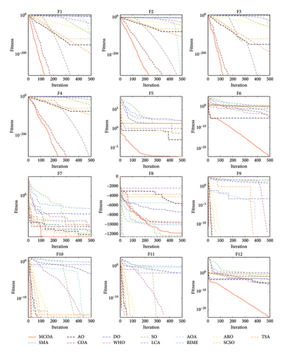
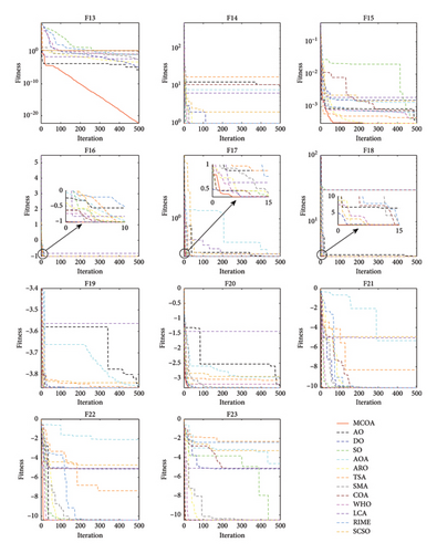
Figure 9 presents the convergence curves of MCOA compared with other algorithms across all 23 benchmark functions. The results demonstrate that MCOA can continuously converge to the optimal solution within 500 iterations in most test cases. For unimodal functions, while MCOA, COA, and SMA all reach the optimal value (0) on F1∼F4, MCOA requires notably fewer iterations, indicating superior convergence speed. This acceleration can be attributed primarily to the Lévy flight operator, which enhances the exploitation phase and guides the algorithm more efficiently toward the global optimum. For the more challenging F5 and F6, the convergence curves of MCOA exhibit steady decay with continuously improving solution accuracy. In contrast, the other comparison algorithms stagnate earlier. On F7, MCOA is slightly inferior in the initial iterations but eventually obtains better convergence results than other optimizers. For multimodal functions, MCOA rapidly identifies promising regions during early iterations and intensively exploits these neighborhoods to enhance convergence accuracy. On F9∼F11, MCOA provides desirable high-quality solutions with minimal iterations. MCOA inherits the superior exploration capability of AO due to the fusion of the position update mode of expanded exploration. On F12 and F13, the exploration performance of MCOA and AO in the early iterations is almost similar, but the former demonstrates superior local optima avoidance, ensuring better convergence accuracy. On F8, MCOA performs slightly worse than SO and SMA, ranking third in the test. For fixed-dimension multimodal functions, MCOA also maintains good convergence speed and accuracy. It can be found that MCOA rapidly transitions from exploration to exploitation in the initial iteration, effectively circumventing local optima. Particularly on F14, F15, F22, and F23, COA visibly falls into local optima due to imbalance between exploration and exploitation—a problem that MCOA successfully overcomes. The above experimental results indicate that the four improvement steps adopted in this paper strengthen the algorithm’s exploitation and exploration, allowing it to converge more rapidly to higher accuracy and avoid local stagnation in the optimization process. In summary, MCOA achieves highly competitive convergence performance compared to other state-of-the-art MH algorithms.
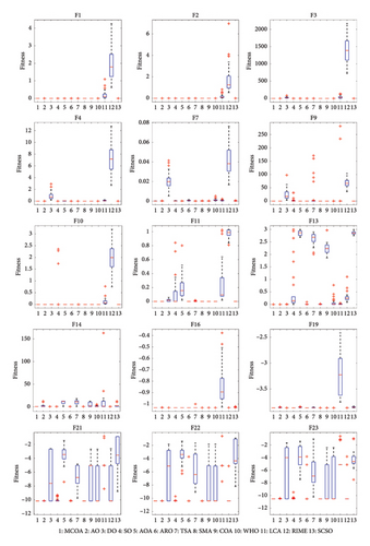
5.2.6. Boxplot Behavior Analysis
Figure 10 presents the boxplot of MCOA and comparison algorithms on partial benchmark functions. In these boxplots, the center line represents the median value, while the upper and lower whisker edges indicate maximum and minimum values, respectively, with outliers denoted by plus signs (“+”). From the results, MCOA shows good data consistency on unimodal functions F1, F2, F3, F4, and F7. Notably, on F7, both AO and COA generate outliers, while MCOA does not. Since multimodal and fixed-dimension multimodal functions have local minima, this is a stability check for the optimizer. MCOA presents a few outliers on F13, but the other algorithms are not as satisfactory, with obvious outliers for SO, and the medians of TSA and COA are far from the theoretical optimum (0). In other test cases, the boxplots of MCOA are more centralized than comparison algorithms in terms of maximum, minimum, and median values. These boxplot analyses confirm that the integration of multiple search strategies significantly improves the robustness of COA.
5.2.7. Scalability Analysis
The problem dimension represents the number of independent decision variables to be considered in the optimization problem. As problem dimension increases, many algorithms suffer from dimensional catastrophe, experiencing significant degradation in convergence accuracy. To assess dimensional robustness, we extend the dimension (D) of 13 benchmark functions (F1∼F13) from 30 to 50, 100, 500, and 1000, respectively, with other parameter settings remaining unchanged. The detailed experimental results are presented in Tables 6, 7, 8, and 9.
| Function | Metric | MCOA | AO | DO | SO | AOA | ARO | TSA | SMA | COA | WHO | LCA | RIME | SCSO |
|---|---|---|---|---|---|---|---|---|---|---|---|---|---|---|
| F1 | Mean | 0 | 7.7349E − 104 | 2.2841E − 03 | 3.7615E − 88 | 2.5430E − 04 | 2.3024E − 64 | 1.8368E − 185 | 0 | 0 | 9.0793E − 40 | 1.8894E − 01 | 1.9083E + 01 | 6.7692E − 117 |
| Std | 0 | 4.2358E − 103 | 1.0956E − 03 | 1.4491E − 87 | 8.9585E − 04 | 9.3060E − 64 | 0 | 0 | 0 | 2.8325E − 39 | 2.4430E − 01 | 5.0240E + 00 | 3.3274E − 116 | |
| F2 | Mean | 0 | 4.2901E − 50 | 2.1083E − 02 | 3.4499E − 39 | 2.4315E − 186 | 3.7916E − 35 | 1.1161E − 95 | 0 | 0 | 1.1617E − 22 | 2.5103E − 01 | 9.6854E + 00 | 2.3729E − 59 |
| Std | 0 | 1.7196E − 49 | 5.1066E − 03 | 5.2408E − 39 | 0 | 1.1433E − 34 | 2.5455E − 95 | 0 | 0 | 2.2054E − 22 | 1.6048E − 01 | 3.5615E + 00 | 1.1698E − 58 | |
| F3 | Mean | 0 | 1.5405E − 104 | 1.1544E + 03 | 2.0839E − 52 | 7.7499E − 02 | 5.5181E − 46 | 1.8650E − 174 | 0 | 0 | 3.8369E − 20 | 1.4141E + 02 | 1.4235E + 04 | 1.5770E − 110 |
| Std | 0 | 8.4251E − 104 | 6.3811E + 02 | 9.0553E − 52 | 6.4032E − 02 | 2.4178E − 45 | 0 | 0 | 0 | 1.1419E − 19 | 1.6365E + 02 | 2.6278E + 03 | 7.3573E − 110 | |
| F4 | Mean | 0 | 2.2620E − 56 | 1.5925E + 01 | 2.2015E − 38 | 5.5102E − 02 | 5.5789E − 25 | 1.7409E − 87 | 0 | 0 | 5.3149E − 15 | 9.0639E − 02 | 3.2034E + 01 | 1.2047E − 57 |
| Std | 0 | 1.2098E − 55 | 6.8298E + 00 | 4.7433E − 38 | 9.7968E − 03 | 2.1152E − 24 | 8.7894E − 87 | 0 | 0 | 1.2580E − 14 | 6.1348E − 02 | 5.4084E + 00 | 4.7629E − 57 | |
| F5 | Mean | 6.5146E − 08 | 2.2281E − 03 | 2.6482E + 01 | 9.0498E + 00 | 1.6269E + 01 | 1.3554E − 01 | 1.6186E + 01 | 4.4411E + 00 | 1.5860E + 01 | 1.6144E + 01 | 1.0536E + 00 | 6.9548E + 02 | 1.6306E + 01 |
| Std | 1.6391E − 07 | 6.9299E − 03 | 1.8210E + 01 | 1.7317E + 01 | 2.3323E + 01 | 2.7514E − 01 | 2.3282E + 01 | 1.2213E + 01 | 2.2818E + 01 | 2.3371E + 01 | 3.1476E + 00 | 1.0962E + 03 | 2.3454E + 01 | |
| F6 | Mean | 4.6773E − 17 | 3.3897E − 04 | 1.0637E − 03 | 5.2073E + 00 | 7.2754E + 00 | 5.5860E − 02 | 1.1075E + 01 | 3.6408E − 02 | 2.4550E + 00 | 5.1673E − 01 | 2.6528E − 01 | 1.8307E + 01 | 4.8530E + 00 |
| Std | 2.3449E − 16 | 8.4400E − 04 | 3.9624E − 04 | 4.7520E + 00 | 3.6447E − 01 | 5.6515E − 02 | 8.0492E − 01 | 2.7966E − 02 | 6.7714E − 01 | 5.1087E − 01 | 3.8861E − 01 | 4.5393E + 00 | 8.6371E − 01 | |
| F7 | Mean | 5.5914E − 05 | 1.1463E − 04 | 5.2070E − 02 | 2.1473E − 04 | 7.0890E − 05 | 6.9430E − 04 | 7.6761E − 05 | 2.0777E − 04 | 6.8026E − 05 | 1.2825E − 03 | 1.0858E − 03 | 1.4042E − 01 | 1.4376E − 04 |
| Std | 4.1994E − 05 | 1.0774E − 04 | 2.1278E − 02 | 2.4099E − 04 | 7.3905E − 05 | 4.9112E − 04 | 6.1382E − 05 | 1.8227E − 04 | 8.9522E − 05 | 1.0268E − 03 | 9.5761E − 04 | 3.5595E − 02 | 1.7278E − 04 | |
| F8 | Mean | −2.0854E + 04 | −9.7195E + 03 | −1.1501E + 04 | −1.7331E + 04 | −6.7910E + 03 | −1.4599E + 04 | −4.5282E + 03 | −2.0948E + 04 | −1.2938E + 04 | −1.3485E + 04 | −1.6320E + 04 | −1.5286E + 04 | −8.1440E + 03 |
| Std | 1.2508E + 02 | 6.0323E + 03 | 8.9620E + 02 | 1.6049E + 03 | 4.8902E + 02 | 7.3064E + 02 | 7.1793E + 02 | 1.3306E + 00 | 8.0954E + 02 | 7.1133E + 02 | 6.8184E + 03 | 7.0800E + 02 | 1.4347E + 03 | |
| F9 | Mean | 0 | 0 | 6.4524E + 01 | 1.0405E + 01 | 0 | 0 | 1.9914E + 01 | 0 | 0 | 1.8948E − 15 | 1.3293E + 01 | 1.3930E + 02 | 0 |
| Std | 0 | 0 | 4.4011E + 01 | 1.8069E + 01 | 0 | 0 | 7.5242E + 01 | 0 | 0 | 1.0378E − 14 | 7.1894E + 01 | 3.4050E + 01 | 0 | |
| F10 | Mean | 8.8818E − 16 | 8.8818E − 16 | 7.9761E − 03 | 4.4409E − 15 | 8.8818E − 16 | 8.8818E − 16 | 4.7962E − 15 | 8.8818E − 16 | 8.8818E − 16 | 1.1250E − 15 | 7.7834E − 02 | 3.4887E + 00 | 8.8818E − 16 |
| Std | 0 | 0 | 2.5504E − 03 | 0 | 0 | 0 | 1.0840E − 15 | 0 | 0 | 9.0135E − 16 | 6.5108E − 02 | 6.5645E − 01 | 0 | |
| F11 | Mean | 0 | 0 | 1.2615E − 02 | 0 | 1.2803E + 00 | 0 | 1.2716E − 03 | 0 | 0 | 0 | 3.4969E − 01 | 1.1670E + 00 | 0 |
| Std | 0 | 0 | 9.2954E − 03 | 0 | 7.1519E − 01 | 0 | 3.9465E − 03 | 0 | 0 | 0 | 3.1320E − 01 | 3.9062E − 02 | 0 | |
| F12 | Mean | 2.3110E − 16 | 7.1745E − 06 | 5.6873E − 01 | 1.8121E − 02 | 7.3251E − 01 | 1.8136E − 03 | 1.0910E + 00 | 8.7114E − 03 | 5.9790E − 02 | 3.8242E − 02 | 1.0904E − 03 | 1.2911E + 01 | 2.5462E − 01 |
| Std | 9.2021E − 16 | 1.6101E − 05 | 8.9093E − 01 | 3.3598E − 02 | 3.3961E − 02 | 2.2797E − 03 | 1.8066E − 01 | 1.4214E − 02 | 3.0410E − 02 | 6.6049E − 02 | 1.8913E − 03 | 4.5507E + 00 | 7.1510E − 02 | |
| F13 | Mean | 1.8847E − 16 | 2.4919E − 05 | 1.1670E + 00 | 9.4552E − 01 | 4.8593E + 00 | 3.8725E − 02 | 4.6255E + 00 | 2.0973E − 02 | 4.4649E + 00 | 6.3355E − 01 | 1.5807E − 02 | 2.1164E + 01 | 4.8952E + 00 |
| Std | 8.9931E − 16 | 3.2048E − 05 | 6.0269E + 00 | 1.4892E + 00 | 1.1625E − 01 | 4.8008E − 02 | 3.1825E − 01 | 2.5517E − 02 | 3.4891E − 01 | 3.8080E − 01 | 2.5403E − 02 | 2.5321E + 01 | 5.1733E − 02 | |
- Note: The best results obtained are highlighted in bold.
| Function | Metric | MCOA | AO | DO | SO | AOA | ARO | TSA | SMA | COA | WHO | LCA | RIME | SCSO |
|---|---|---|---|---|---|---|---|---|---|---|---|---|---|---|
| F1 | Mean | 0 | 1.0280E − 100 | 7.9950E − 01 | 2.0383E − 81 | 2.3447E − 02 | 1.0462E − 58 | 3.8389E − 176 | 0 | 0 | 1.1250E − 34 | 4.2667E − 01 | 3.8142E + 02 | 7.5297E − 113 |
| Std | 0 | 5.6305E − 100 | 2.9849E − 01 | 7.3667E − 81 | 9.3871E − 03 | 3.6205E − 58 | 0 | 0 | 0 | 5.4149E − 34 | 6.6864E − 01 | 7.6212E + 01 | 4.1007E − 112 | |
| F2 | Mean | 0 | 3.6125E − 50 | 4.6184E − 01 | 1.2834E − 35 | 3.5570E − 57 | 5.4971E − 34 | 1.0145E − 90 | 0 | 0 | 7.9306E + 00 | 6.0802E − 01 | 8.1899E + 01 | 7.8695E − 59 |
| Std | 0 | 1.4726E − 49 | 6.9436E − 02 | 1.1444E − 35 | 1.9051E − 56 | 1.4422E − 33 | 1.5057E − 90 | 0 | 0 | 4.3437E + 01 | 4.8738E − 01 | 1.6426E + 01 | 2.5259E − 58 | |
| F3 | Mean | 0 | 1.8293E − 103 | 2.8873E + 04 | 8.9938E − 28 | 2.8475E + 03 | 2.2876E − 45 | 1.1240E − 166 | 0 | 0 | 7.7615E − 16 | 1.2417E + 03 | 9.7591E + 04 | 9.6461E − 109 |
| Std | 0 | 1.0012E − 102 | 9.5236E + 03 | 4.9261E − 27 | 1.5593E + 04 | 1.0221E − 44 | 0 | 0 | 0 | 2.6433E − 15 | 1.2857E + 03 | 1.4764E + 04 | 5.2613E − 108 | |
| F4 | Mean | 0 | 2.8275E − 51 | 5.7611E + 01 | 1.3116E − 36 | 9.1657E − 02 | 1.2094E − 24 | 2.7756E − 84 | 0 | 0 | 2.6653E − 13 | 8.5062E − 02 | 6.1159E + 01 | 3.3397E − 56 |
| Std | 0 | 1.5476E − 50 | 8.4975E + 00 | 2.1253E − 36 | 1.4551E − 02 | 5.3540E − 24 | 3.2852E − 84 | 0 | 0 | 4.6102E − 13 | 5.2885E − 02 | 6.1479E + 00 | 1.6400E − 55 | |
| F5 | Mean | 1.1789E − 06 | 7.3024E − 02 | 3.2959E + 02 | 9.8905E + 01 | 9.8909E + 01 | 8.0408E − 01 | 9.8354E + 01 | 4.9957E + 01 | 9.7746E + 01 | 9.7699E + 01 | 4.6839E + 00 | 1.0046E + 05 | 9.8921E + 01 |
| Std | 9.4324E − 07 | 9.8156E − 02 | 4.5907E + 01 | 5.0650E − 02 | 2.5919E − 02 | 2.5957E − 01 | 4.4047E − 01 | 6.8409E + 01 | 2.9123E − 01 | 2.7783E − 01 | 5.4918E + 00 | 6.0071E + 04 | 2.0762E − 02 | |
| F6 | Mean | 1.3574E − 13 | 3.4756E − 04 | 1.2750E + 00 | 1.2831E + 01 | 1.8019E + 01 | 4.5997E − 01 | 2.4394E + 01 | 9.0584E − 01 | 1.0097E + 01 | 5.6031E + 00 | 7.2485E − 01 | 3.6689E + 02 | 1.2577E + 01 |
| Std | 3.9085E − 13 | 7.2419E − 04 | 5.1230E − 01 | 1.0975E + 01 | 6.2769E − 01 | 2.5261E − 01 | 4.3691E − 01 | 9.5606E − 01 | 1.4159E + 00 | 1.3568E + 00 | 1.3895E + 00 | 6.5292E + 01 | 2.2131E + 00 | |
| F7 | Mean | 4.7761E − 05 | 1.2987E − 04 | 2.6727E − 01 | 1.7911E − 04 | 8.6091E − 05 | 6.2538E − 04 | 9.1754E − 05 | 1.9109E − 04 | 9.6381E − 05 | 3.7210E − 03 | 1.0868E − 03 | 1.0376E + 00 | 2.4695E − 04 |
| Std | 3.8300E − 05 | 8.7567E − 05 | 7.3757E − 02 | 1.1022E − 04 | 9.3700E − 05 | 4.7611E − 04 | 8.7116E − 05 | 1.9036E − 04 | 7.7564E − 05 | 1.0246E − 02 | 8.7126E − 04 | 2.7361E − 01 | 3.6582E − 04 | |
| F8 | Mean | −3.7145E + 04 | −1.0295E + 04 | −2.1089E + 04 | −4.1359E + 04 | −1.0143E + 04 | −2.2948E + 04 | −6.1434E + 03 | −4.1891E + 04 | −2.1248E + 04 | −2.1739E + 04 | −2.6082E + 04 | −2.6405E + 04 | −1.8223E + 04 |
| Std | 5.8996E + 03 | 2.2147E + 03 | 1.9093E + 03 | 1.0173E + 03 | 7.4680E + 02 | 9.8218E + 02 | 7.3868E + 02 | 8.1244E + 00 | 2.7163E + 03 | 1.6436E + 03 | 3.1647E + 03 | 1.2346E + 03 | 2.6373E + 03 | |
| F9 | Mean | 0 | 0 | 1.9800E + 02 | 2.2757E + 01 | 0 | 0 | 5.6857E − 01 | 0 | 0 | 0 | 2.9308E + 01 | 4.6844E + 02 | 0 |
| Std | 0 | 0 | 1.1546E + 02 | 4.0890E + 01 | 0 | 0 | 5.7831E − 01 | 0 | 0 | 0 | 1.5914E + 02 | 5.8863E + 01 | 0 | |
| F10 | Mean | 8.8818E − 16 | 8.8818E − 16 | 9.9230E − 01 | 4.4409E − 15 | 2.6718E − 04 | 8.8818E − 16 | 5.7436E − 15 | 8.8818E − 16 | 8.8818E − 16 | 1.3619E − 15 | 9.7450E − 02 | 6.4514E + 00 | 8.8818E − 16 |
| Std | 0 | 0 | 6.4943E − 01 | 0 | 8.2538E − 04 | 0 | 1.7413E − 15 | 0 | 0 | 1.2283E − 15 | 1.3268E − 01 | 1.1928E + 00 | 0 | |
| F11 | Mean | 0 | 0 | 4.3361E − 01 | 0 | 5.9488E + 02 | 0 | 1.0693E − 03 | 0 | 0 | 0 | 3.6712E − 01 | 4.4507E + 00 | 0 |
| Std | 0 | 0 | 1.1933E − 01 | 0 | 1.4759E + 02 | 0 | 3.3703E − 03 | 0 | 0 | 0 | 2.9811E − 01 | 6.9416E − 01 | 0 | |
| F12 | Mean | 5.1195E − 14 | 9.2978E − 07 | 4.3135E + 00 | 1.5198E − 01 | 9.0474E − 01 | 6.9506E − 03 | 1.2246E + 00 | 1.7697E − 02 | 2.2540E − 01 | 8.2441E − 02 | 5.8482E − 04 | 3.6685E + 02 | 3.3567E − 01 |
| Std | 1.2882E − 13 | 1.6679E − 06 | 1.8361E + 00 | 3.5096E − 01 | 2.2806E − 02 | 3.8724E − 03 | 7.8149E − 02 | 4.6295E − 02 | 5.2620E − 02 | 3.6325E − 02 | 1.2302E − 03 | 7.9056E + 02 | 9.9947E − 02 | |
| F13 | Mean | 1.7144E − 11 | 4.9527E − 05 | 9.1214E + 01 | 1.4810E + 00 | 9.9663E + 00 | 2.5081E − 01 | 9.7899E + 00 | 4.3329E − 01 | 9.5430E + 00 | 4.8490E + 00 | 3.1294E − 02 | 5.4596E + 03 | 9.9077E + 00 |
| Std | 9.1529E − 11 | 1.2352E − 04 | 2.1356E + 01 | 2.9277E + 00 | 5.7282E − 02 | 1.8847E − 01 | 7.8983E − 02 | 8.3778E − 01 | 2.9732E − 01 | 1.0141E + 00 | 4.1138E − 02 | 5.8103E + 03 | 4.9238E − 02 | |
- Note: The best results obtained are highlighted in bold.
| Function | Metric | MCOA | AO | DO | SO | AOA | ARO | TSA | SMA | COA | WHO | LCA | RIME | SCSO |
|---|---|---|---|---|---|---|---|---|---|---|---|---|---|---|
| F1 | Mean | 0 | 2.3744E − 101 | 8.1243E + 03 | 8.4588E − 71 | 6.3288E − 01 | 2.4095E − 56 | 2.9656E − 162 | 0 | 0 | 1.9023E − 30 | 1.5815E + 00 | 1.6775E + 05 | 2.3021E − 110 |
| Std | 0 | 1.3005E − 100 | 1.5910E + 03 | 3.2087E − 70 | 3.7477E − 02 | 1.0544E − 55 | 2.2228E − 162 | 0 | 0 | 5.2800E − 30 | 2.1952E + 00 | 1.1056E + 04 | 1.0652E − 109 | |
| F2 | Mean | 0 | 9.3901E − 54 | 6.8703E + 01 | 1.0861E − 31 | 1.1772E − 03 | 8.8065E − 31 | 8.1518E − 83 | 0 | 0 | 5.9576E + 02 | 3.6523E + 00 | 7.7462E + 126 | 3.1856E − 57 |
| Std | 0 | 5.1432E − 53 | 7.1143E + 00 | 1.1724E − 31 | 1.4740E − 03 | 4.1447E − 30 | 3.8002E − 83 | 0 | 0 | 6.1850E + 02 | 2.3513E + 00 | 4.2427E + 127 | 1.2001E − 56 | |
| F3 | Mean | 0 | 3.1524E − 98 | 1.5436E + 06 | 3.4130E − 05 | 3.8224E + 01 | 3.5641E − 40 | 9.8772E − 154 | 0 | 0 | 6.2555E − 09 | 1.8917E + 05 | 2.6453E + 06 | 2.6823E − 101 |
| Std | 0 | 1.7263E − 97 | 2.2355E + 05 | 1.8694E − 04 | 2.2731E + 01 | 1.0371E − 39 | 4.3541E − 153 | 0 | 0 | 2.5091E − 08 | 3.1723E + 05 | 2.3395E + 05 | 1.3565E − 100 | |
| F4 | Mean | 0 | 1.1188E − 54 | 9.4454E + 01 | 1.0073E − 33 | 1.7824E − 01 | 1.0994E − 22 | 1.4261E − 72 | 0 | 0 | 4.6768E − 10 | 6.5452E − 02 | 9.3386E + 01 | 8.5877E − 56 |
| Std | 0 | 5.6234E − 54 | 1.0581E + 00 | 1.4463E − 33 | 1.7090E − 02 | 2.1659E − 22 | 5.4324E − 72 | 0 | 0 | 9.4550E − 10 | 4.4775E − 02 | 1.3180E + 00 | 2.0815E − 55 | |
| F5 | Mean | 1.2293E − 03 | 8.8272E − 03 | 2.7993E + 06 | 3.4978E + 01 | 5.0067E + 01 | 4.9994E − 01 | 4.9795E + 01 | 4.4006E + 00 | 4.9791E + 01 | 4.9805E + 01 | 2.9965E + 00 | 2.9534E + 07 | 4.9891E + 01 |
| Std | 5.9729E − 04 | 2.9949E − 02 | 9.2405E + 06 | 1.2647E + 02 | 1.5222E + 02 | 2.2133E + 00 | 1.5194E + 02 | 1.7868E + 01 | 1.5193E + 02 | 1.5197E + 02 | 1.0833E + 01 | 9.1780E + 07 | 1.5223E + 02 | |
| F6 | Mean | 8.0148E − 06 | 9.6038E − 04 | 8.5352E + 03 | 7.7803E + 01 | 1.1570E + 02 | 4.9114E + 00 | 1.2475E + 02 | 3.0361E + 01 | 9.6308E + 01 | 1.0190E + 02 | 3.8864E + 00 | 1.6333E + 05 | 6.7263E + 01 |
| Std | 4.2639E − 05 | 1.6115E − 03 | 1.9899E + 03 | 5.5978E + 01 | 1.5632E + 00 | 2.6064E + 00 | 1.6187E − 07 | 3.4732E + 01 | 3.7897E + 00 | 1.7087E + 01 | 5.7391E + 00 | 1.2908E + 04 | 1.3626E + 01 | |
| F7 | Mean | 4.6361E − 05 | 9.2061E − 05 | 1.1322E + 02 | 1.5806E − 04 | 8.2912E − 05 | 6.6465E − 04 | 9.6236E − 05 | 4.2955E − 04 | 8.3841E − 05 | 2.3331E − 03 | 1.8407E − 03 | 2.0583E + 03 | 2.0571E − 04 |
| Std | 4.0052E − 05 | 8.2948E − 05 | 6.3092E + 01 | 1.3657E − 04 | 7.2410E − 05 | 3.7044E − 04 | 8.1436E − 05 | 4.7865E − 04 | 8.7382E − 05 | 2.8136E − 03 | 1.4878E − 03 | 2.9274E + 02 | 1.9281E − 04 | |
| F8 | Mean | −9.1981E + 04 | −3.9134E + 04 | −7.1601E + 04 | −2.0759E + 05 | −2.2898E + 04 | −5.9284E + 04 | −1.3928E + 04 | −2.0937E + 05 | −6.3220E + 04 | −5.8392E + 04 | −1.8771E + 05 | −8.0364E + 04 | −6.7276E + 04 |
| Std | 1.0236E + 04 | 1.2275E + 04 | 4.4140E + 03 | 5.4426E + 03 | 1.5879E + 03 | 2.8486E + 03 | 2.1406E + 03 | 2.5433E + 02 | 7.0133E + 03 | 6.9569E + 03 | 2.9000E + 04 | 3.3878E + 03 | 2.8645E + 04 | |
| F9 | Mean | 0 | 0 | 2.3689E + 03 | 1.0380E − 01 | 6.7740E − 06 | 0 | 5.6790E − 01 | 0 | 0 | 9.2678E − 11 | 1.7992E + 00 | 5.4725E + 03 | 0 |
| Std | 0 | 0 | 6.2821E + 02 | 5.6853E − 01 | 7.7056E − 06 | 0 | 6.3274E − 01 | 0 | 0 | 5.0762E − 10 | 3.3375E + 00 | 1.6879E + 02 | 0 | |
| F10 | Mean | 8.8818E − 16 | 8.8818E − 16 | 6.7017E + 00 | 5.3883E − 15 | 7.9296E − 03 | 8.8818E − 16 | 6.9278E − 15 | 8.8818E − 16 | 8.8818E − 16 | 1.9540E − 15 | 1.2997E − 01 | 2.0334E + 01 | 8.8818E − 16 |
| Std | 0 | 0 | 5.5563E − 01 | 1.5979E − 15 | 3.7008E − 04 | 0 | 1.6559E − 15 | 0 | 0 | 2.3137E − 15 | 2.0514E − 01 | 1.1825E − 01 | 0 | |
| F11 | Mean | 0 | 0 | 7.4133E + 01 | 0 | 9.9981E + 03 | 0 | 3.2886E − 04 | 0 | 0 | 0 | 3.7696E − 01 | 1.4915E + 03 | 0 |
| Std | 0 | 0 | 1.5202E + 01 | 0 | 2.8089E + 03 | 0 | 1.8012E − 03 | 0 | 0 | 0 | 3.6867E − 01 | 1.0662E + 02 | 0 | |
| F12 | Mean | 5.7937E − 07 | 1.6036E − 05 | 1.2025E + 07 | 7.3927E − 02 | 1.0818E + 00 | 1.3846E − 02 | 1.1987E + 00 | 6.6236E − 03 | 7.3447E − 01 | 8.1462E − 01 | 3.1149E − 04 | 3.6313E + 08 | 2.7103E − 01 |
| Std | 1.1181E − 06 | 5.7879E − 05 | 9.8827E + 06 | 1.7681E − 01 | 1.3998E − 02 | 4.9426E − 03 | 1.1450E − 02 | 1.6565E − 02 | 4.9539E − 02 | 2.8525E − 01 | 4.5977E − 04 | 9.4372E + 07 | 1.1045E − 01 | |
| F13 | Mean | 2.5584E − 04 | 7.2447E − 01 | 4.9499E + 07 | 6.1562E + 00 | 5.0199E + 01 | 3.2535E + 00 | 4.9781E + 01 | 3.2755E + 00 | 4.9827E + 01 | 5.5996E + 01 | 1.1724E − 01 | 1.0275E + 09 | 4.9921E + 01 |
| Std | 3.3881E − 04 | 3.9553E + 00 | 4.0576E + 07 | 1.2724E + 01 | 2.9298E − 02 | 2.2001E + 00 | 4.4677E − 02 | 5.2037E + 00 | 8.9446E − 02 | 6.2152E + 00 | 1.7994E − 01 | 2.3270E + 08 | 5.0976E − 02 | |
- Note: The best results obtained are highlighted in bold.
| Function | Metric | MCOA | AO | DO | SO | AOA | ARO | TSA | SMA | COA | WHO | LCA | RIME | SCSO |
|---|---|---|---|---|---|---|---|---|---|---|---|---|---|---|
| F1 | Mean | 0 | 2.9856E − 114 | 6.9734E + 04 | 4.0431E − 68 | 1.7139E + 00 | 5.9681E − 52 | 1.6650E − 158 | 0 | 0 | 1.9864E − 28 | 6.2498E + 00 | 9.1920E + 05 | 8.1506E − 111 |
| Std | 0 | 1.2213E − 113 | 1.3863E + 04 | 8.1175E − 68 | 7.7934E − 02 | 3.2656E − 51 | 1.0787E − 158 | 0 | 0 | 8.0535E − 28 | 9.6729E + 00 | 3.6115E + 04 | 2.4952E − 110 | |
| F2 | Mean | 0 | 2.3557E − 61 | Inf | 3.2339E − 19 | 1.2806E − 02 | 6.1098E − 30 | 9.9162E − 82 | 0 | 0 | 2.0554E + 03 | 5.1278E + 00 | 2.6852E + 03 | 4.1971E − 57 |
| Std | 0 | 1.2903E − 60 | NaN | 1.7713E − 18 | 6.1394E − 03 | 1.8666E − 29 | 2.5170E − 82 | 0 | 0 | 1.2702E + 03 | 2.7949E + 00 | 8.8150E + 01 | 1.0828E − 56 | |
| F3 | Mean | 0 | 1.2666E − 99 | 5.9197E + 06 | 2.6098E − 09 | 1.2807E + 02 | 1.0508E − 36 | 3.3140E − 149 | 0 | 0 | 5.7899E − 07 | 9.7056E + 05 | 1.0094E + 07 | 2.5537E − 99 |
| Std | 0 | 5.2244E − 99 | 7.9554E + 05 | 1.4294E − 08 | 5.1991E + 01 | 4.7374E − 36 | 9.0341E − 149 | 0 | 0 | 2.2652E − 06 | 1.0762E + 06 | 8.4913E + 05 | 1.3983E − 98 | |
| F4 | Mean | 0 | 1.2448E − 52 | 9.7598E + 01 | 7.4351E − 33 | 2.0877E − 01 | 4.3472E − 21 | 7.3046E + 01 | 0 | 0 | 1.6475E − 09 | 7.8676E − 02 | 9.7218E + 01 | 8.9408E − 55 |
| Std | 0 | 6.7095E − 52 | 6.1092E − 01 | 1.0810E − 32 | 1.1437E − 02 | 8.3507E − 21 | 4.4802E + 01 | 0 | 0 | 3.7722E − 09 | 6.0081E − 02 | 5.9586E − 01 | 3.0806E − 54 | |
| F5 | Mean | 9.9478E − 03 | 8.6190E − 01 | 3.4927E + 07 | 6.6595E + 01 | 6.6814E + 01 | 6.9687E + 00 | 1.3623E + 02 | 9.8887E + 02 | 6.6510E + 01 | 4.8785E + 02 | 1.9824E + 00 | 2.0434E + 08 | 6.6596E + 01 |
| Std | 4.8714E − 02 | 4.5925E + 00 | 1.3344E + 08 | 2.5344E + 02 | 2.5347E + 02 | 3.5182E + 01 | 2.3791E + 02 | 0 | 2.5311E + 02 | 2.4902E + 03 | 8.4931E + 00 | 7.7791E + 08 | 2.5344E + 02 | |
| F6 | Mean | 7.7946E − 03 | 1.1170E − 03 | 7.2787E + 04 | 1.0647E + 02 | 2.4278E + 02 | 9.9086E + 00 | 2.4975E + 02 | 3.2849E + 01 | 2.1427E + 02 | 2.2599E + 02 | 5.9813E + 00 | 9.1347E + 05 | 1.3999E + 02 |
| Std | 4.0913E − 02 | 1.4630E − 03 | 1.0785E + 04 | 1.0651E + 02 | 1.2542E + 00 | 5.1747E + 00 | 1.7640E − 07 | 4.9734E + 01 | 3.4013E + 00 | 2.2909E + 01 | 1.1349E + 01 | 5.3172E + 04 | 2.6253E + 01 | |
| F7 | Mean | 5.0377E − 05 | 6.9669E − 05 | 5.0945E + 03 | 2.3111E − 04 | 1.2346E − 04 | 7.5169E − 04 | 9.6673E − 05 | 4.5623E − 04 | 8.0742E − 05 | 3.0568E − 03 | 3.7797E − 03 | 3.6246E + 04 | 2.1985E − 04 |
| Std | 3.9966E − 05 | 5.2334E − 05 | 2.0012E + 03 | 1.8875E − 04 | 1.2029E − 04 | 5.4362E − 04 | 8.8095E − 05 | 3.9299E − 04 | 7.8869E − 05 | 5.2683E − 03 | 4.1201E − 03 | 3.7503E + 03 | 2.4883E − 04 | |
| F8 | Mean | −1.8649E + 05 | −6.3931E + 04 | −1.1067E + 05 | −4.1467E + 05 | −3.2143E + 04 | −8.4126E + 04 | −1.8174E + 04 | −4.1883E + 05 | −9.2424E + 04 | −8.5749E + 04 | −3.7138E + 05 | −1.1547E + 05 | −1.0885E + 05 |
| Std | 2.3285E + 04 | 1.9424E + 04 | 7.5454E + 03 | 7.4849E + 03 | 2.0424E + 03 | 3.4652E + 03 | 2.2270E + 03 | 2.4606E + 02 | 1.0548E + 04 | 8.2143E + 03 | 5.9020E + 04 | 4.5758E + 03 | 2.8701E + 04 | |
| F9 | Mean | 0 | 0 | 5.3688E + 03 | 0 | 6.1114E − 05 | 0 | 3.3166E − 01 | 0 | 0 | 0 | 4.1184E + 00 | 1.3083E + 04 | 0 |
| Std | 0 | 0 | 5.1535E + 02 | 0 | 1.1845E − 05 | 0 | 4.7706E − 01 | 0 | 0 | 0 | 6.8399E + 00 | 2.1376E + 02 | 0 | |
| F10 | Mean | 8.8818E − 16 | 8.8818E − 16 | 1.0178E + 01 | 5.6251E − 15 | 9.2845E − 03 | 8.8818E − 16 | 7.7568E − 15 | 8.8818E − 16 | 8.8818E − 16 | 1.9540E − 15 | 1.0204E − 01 | 2.0707E + 01 | 8.8818E − 16 |
| Std | 0 | 0 | 5.7536E − 01 | 1.7034E − 15 | 2.6316E − 04 | 0 | 9.0135E − 16 | 0 | 0 | 1.6559E − 15 | 8.8998E − 02 | 3.9470E − 02 | 0 | |
| F11 | Mean | 0 | 0 | 6.6670E + 02 | 0 | 2.8268E + 04 | 0 | 9.5962E − 04 | 0 | 0 | 0 | 3.5079E − 01 | 8.1906E + 03 | 0 |
| Std | 0 | 0 | 1.0499E + 02 | 0 | 4.6720E + 02 | 0 | 3.9108E − 03 | 0 | 0 | 0 | 2.7062E − 01 | 4.0529E + 02 | 0 | |
| F12 | Mean | 9.8660E − 07 | 4.6628E − 03 | 1.2437E + 09 | 1.3509E − 01 | 1.1135E + 00 | 1.2893E − 02 | 1.1892E + 00 | 7.7567E − 03 | 9.0452E − 01 | 1.0110E + 00 | 3.6746E − 04 | 4.9373E + 09 | 3.3791E − 01 |
| Std | 1.9961E − 06 | 8.9320E − 03 | 4.3081E + 08 | 3.5732E − 01 | 5.6980E − 03 | 6.2962E − 03 | 4.4934E − 03 | 1.7256E − 02 | 4.0259E − 02 | 3.9321E − 01 | 7.0352E − 04 | 6.9890E + 08 | 1.0353E − 01 | |
| F13 | Mean | 7.7431E − 04 | 1.0156E + 01 | 1.8911E + 09 | 2.3274E + 01 | 1.0050E + 02 | 4.3517E + 00 | 9.9737E + 01 | 2.6675E + 00 | 9.9841E + 01 | 1.1425E + 02 | 1.5162E − 01 | 1.0663E + 10 | 9.9953E + 01 |
| Std | 1.2910E − 03 | 2.6512E + 01 | 6.1879E + 08 | 3.9863E + 01 | 5.0436E − 02 | 3.4150E + 00 | 4.7262E − 02 | 4.7089E + 00 | 2.3647E − 02 | 1.2634E + 01 | 2.6270E − 01 | 1.2335E + 09 | 4.3439E − 02 | |
- Note: The best results obtained are highlighted in bold.
Based on the data in Tables 6, 7, 8, and 9, MCOA achieves the optimal performance on 12 out of 13 50-dimensional problems (92.31%), substantially outperforming SMA (61.54%), COA (53.85%), AO (23.08%), ARO (23.08%), SCSO (23.08%), AOA (15.38%), SO (7.69%), and WHO (7.69%). For 100-dimensional problems, MCOA provides the best mean fitness and standard deviation results on 12 out of 13 (92.31%), higher than SMA (61.54%), COA (53.85%), AO (23.08%), ARO (23.08%), SCSO (23.08%), WHO (15.38%), SO (7.69%), and AOA (7.69%). For 500-dimensional problems, MCOA performs best on 12 out of 13 (92.31%), higher than SMA (61.54%), COA (53.85%), AO (23.08%), ARO (23.08%), SCSO (23.08%), SO (7.69%), and WHO (7.69%). Besides, in the extreme case of 1000 dimensions, MCOA shows the optimal performance on 11 out of 13 (84.62%), higher than SMA (61.54%), COA (53.85%), AO (30.77%), ARO (23.08%), SCSO (23.08%), SO (15.38%), and WHO (15.38%).
Regardless of the dimension extension, MCOA consistently delivers superior quality solutions on F5, F7, F12, and F13. SMA also performs very competitively, consistently ranking first on F8, ahead of MCOA. COA performs the same as MCOA on F1, F2, F3, F4, F9, F10, and F11, but the gap between them is still evident in other cases. Overall, MCOA provides reliable results with good convergence accuracy, even in the face of high-dimensional optimization tasks. Figure 11 illustrates the Friedman mean ranking of MCOA on the different dimensional benchmark functions. MCOA outperforms competitor algorithms by obtaining the ranking values of 1.0769, 1.1538, 1.2308, and 1.3077 for each dimension, respectively. This is because the specular reflection learning and vertical crossover strategy strengthen the exploration and exploitation of the proposed MCOA so that search agents can more effectively leverage the solution information to converge toward the global optimum in the complex search space.
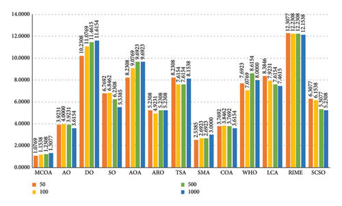
5.3. Comparison With Some Improved Peers on CEC2019 Functions
To further validate the superiority of the suggested optimizer, nine newly proposed improved MH algorithms are selected for comparison with MCOA on the CEC2019 test suite. These algorithms include simplified Aquila optimizer (IAO) [57], dynamic arithmetic optimization algorithm (DAOA) [58], weighted chimp optimization algorithm (WChOA) [59], dynamic multipopulation cooperative sand cat optimizer (DMSCSO) [60], enhanced hybrid arithmetic optimization algorithm (CSOAOA) [61], memetic Harris hawks optimization (EESHHO) [62], hybrid slime arithmetic optimization algorithm (RCLSMAOA) [63], improved hybrid Aquila optimizer and African vulture optimization algorithm (IHAOAVOA) [64], and multistrategy assisted chaotic coot-inspired optimization algorithm (COBHCOOT) [65], and their parameter settings are also consistent with the original literature, as shown in Table 10. All experimental algorithms run independently 30 times on each benchmark problem, and the statistical results obtained are reported in Table 11.
| Algorithm | Year | Parameter value |
|---|---|---|
| IAO | 2022 | U = 0.00565; D1 = 10; ω = 0.005 |
| DAOA | 2022 | α = 25; μ = 0.001 |
| WChOA | 2021 | f = [2.5, 0]; M = Gauss chaptic value |
| DMSCSO | 2023 | G1 ∈ [−1, 1]; SM = 2; rG = [2, 0] |
| CSOAOA | 2022 | α = 5; μ = 0.499; δ ∈ [0.001, 0.01] |
| EESHHO | 2021 | sp ∈ (−1, 1); E0 ∈ (−1, 1) |
| RCLSMAOA | 2023 | z = 0.03; α = 5; μ = 0.499 |
| IHAOAVOA | 2022 | L1 = 0.8; L2 = 0.2; w = 2.5; P2 = 0.4; P3 = 0.6; U = 0.00565; r = 10; ω = 0.005; k = 12000 |
| COBHCOOT | 2022 | a ∈ [2, 0]; obllimit = 40 |
| Function | Metrics | MCOA | IAO | DAOA | WChOA | DMSCSO | CSOAOA | EESHHO | RCLSMAOA | IHAOAVOA | COBHCOOT |
|---|---|---|---|---|---|---|---|---|---|---|---|
| CEC2019-01 | Mean | 4.4645E + 04 | 8.6003E + 04 | 1.1227E + 12 | 4.5689E + 05 | 4.1756E + 04 | 1.4226E + 09 | 4.6614E + 04 | 7.3761E + 09 | 4.6430E + 04 | 1.4625E + 07 |
| Std | 2.7046E + 03 | 2.0261E + 04 | 2.1436E + 12 | 2.5437E + 05 | 2.5833E + 03 | 2.5628E + 09 | 3.1545E + 03 | 3.7828E + 10 | 3.7448E + 03 | 5.0265E + 07 | |
| p value | — | 3.0199E − 11 | 1.4440E − 11 | 3.0199E − 11 | 1.1747E − 04 | 3.0199E − 11 | 1.3832E − 02 | 3.0199E − 11 | 6.5671E − 02 | 6.3560E-05 | |
| Rank | 2 | 5 | 10 | 6 | 1 | 8 | 4 | 9 | 3 | 7 | |
| CEC2019-02 | Mean | 1.7343E + 01 | 1.7640E + 01 | 6.9013E + 02 | 1.7889E + 01 | 1.7343E + 01 | 1.7344E + 01 | 1.7343E + 01 | 1.7512E + 01 | 1.7343E + 01 | 1.7343E + 01 |
| Std | 4.0077E − 08 | 9.7073E − 02 | 2.7209E + 03 | 2.2181E − 01 | 3.0682E − 07 | 1.8588E − 03 | 5.6026E − 06 | 5.1845E − 01 | 9.5813E − 09 | 1.8464E-04 | |
| p value | — | 3.0199E − 11 | 2.3657E − 12 | 3.0199E − 11 | 5.4941E − 11 | 1.1674E − 05 | 3.0199E − 11 | 3.0199E − 11 | 3.0199E − 11 | 3.0199E-11 | |
| Rank | 2 | 8 | 10 | 9 | 3 | 6 | 4 | 7 | 1 | 5 | |
| CEC2019-03 | Mean | 1.2702E + 01 | 1.2704E + 01 | 1.2705E + 01 | 1.2706E + 01 | 1.2702E + 01 | 1.2702E + 01 | 1.2702E + 01 | 1.2705E + 01 | 1.2702E + 01 | 1.2702E + 01 |
| Std | 4.3564E − 12 | 6.6964E − 04 | 1.7414E − 03 | 5.1011E − 03 | 2.3179E − 12 | 6.2840E − 07 | 7.0348E − 08 | 1.4654E − 03 | 5.4143E − 10 | 4.6303E-09 | |
| p value | — | 2.5627E − 11 | 2.5562E − 11 | 2.5627E − 11 | 2.2605E − 02 | 5.1731E − 11 | 3.0799E − 02 | 2.5627E − 11 | 9.6986E − 03 | 2.5627E-11 | |
| Rank | 2 | 7 | 9 | 10 | 1 | 6 | 5 | 8 | 3 | 4 | |
| CEC2019-04 | Mean | 3.6020E + 01 | 4.8204E + 03 | 2.9110E + 04 | 3.0950E + 04 | 1.0100E + 02 | 1.7584E + 02 | 5.8143E + 01 | 4.7296E + 03 | 1.2886E + 02 | 5.2437E + 01 |
| Std | 9.5968E + 00 | 1.5501E + 03 | 9.4946E + 03 | 9.5882E + 03 | 4.8510E + 01 | 1.8824E + 02 | 2.2925E + 01 | 1.0807E + 04 | 6.4910E + 01 | 3.0560E + 01 | |
| p value | — | 3.0199E − 11 | 3.0199E − 11 | 3.0199E − 11 | 1.6132E − 10 | 2.0338E − 09 | 6.2828E − 06 | 5.0114E − 01 | 7.3803E − 10 | 2.7548E-03 | |
| Rank | 1 | 8 | 9 | 10 | 4 | 6 | 3 | 7 | 5 | 2 | |
| CEC2019-05 | Mean | 1.1825E + 00 | 2.6168E + 00 | 7.7139E + 00 | 6.9314E + 00 | 1.1899E + 00 | 1.3907E + 00 | 1.3239E + 00 | 1.6896E + 00 | 1.4996E + 00 | 1.2925E + 00 |
| Std | 4.3591E − 02 | 3.1224E − 01 | 1.6181E + 00 | 8.8225E − 01 | 7.3195E − 02 | 3.7221E − 01 | 2.2619E − 01 | 1.1900E + 00 | 4.1011E − 01 | 1.4050E-01 | |
| p value | — | 3.0199E − 11 | 3.0199E − 11 | 3.0199E − 11 | 7.0617E − 01 | 2.4994E − 03 | 1.1711E − 02 | 5.9706E − 05 | 2.1327E − 05 | 5.3221E-03 | |
| Rank | 1 | 8 | 10 | 9 | 2 | 5 | 4 | 7 | 6 | 3 | |
| CEC2019-06 | Mean | 3.8593E + 00 | 1.1202E + 01 | 1.3773E + 01 | 1.2803E + 01 | 7.8885E + 00 | 4.6271E + 00 | 5.3835E + 00 | 8.7879E + 00 | 5.8631E + 00 | 1.0023E + 01 |
| Std | 1.0623E + 00 | 8.1330E − 01 | 7.3718E − 01 | 9.9492E − 01 | 1.4751E + 00 | 1.4992E + 00 | 5.7356E − 01 | 2.5150E + 00 | 1.2656E + 00 | 8.5608E-01 | |
| p value | — | 3.0199E − 11 | 3.0199E − 11 | 3.0199E − 11 | 7.0881E − 08 | 8.7710E − 02 | 2.1540E − 06 | 8.3520E − 08 | 1.0233E − 01 | 3.0199E-11 | |
| Rank | 1 | 8 | 10 | 9 | 5 | 2 | 3 | 6 | 4 | 7 | |
| CEC2019-07 | Mean | 4.5066E + 01 | 9.9622E + 02 | 1.7216E + 03 | 1.7468E + 03 | 2.3900E + 02 | 3.0158E + 01 | 1.6830E + 02 | 4.1793E + 02 | 3.3148E + 02 | 3.8035E + 02 |
| Std | 9.1662E + 01 | 1.8935E + 02 | 3.4996E + 02 | 2.7445E + 02 | 2.3317E + 02 | 7.2375E + 01 | 1.2917E + 02 | 3.1005E + 02 | 2.1905E + 02 | 1.6057E + 02 | |
| p value | — | 3.0199E − 11 | 3.0199E − 11 | 3.0199E − 11 | 6.7650E − 05 | 3.8710E − 01 | 5.9706E − 05 | 3.6459E − 08 | 4.6856E − 08 | 9.7555E-10 | |
| Rank | 2 | 8 | 9 | 10 | 4 | 1 | 3 | 7 | 5 | 6 | |
| CEC2019-08 | Mean | 4.7709E + 00 | 6.2775E + 00 | 7.4997E + 00 | 7.3817E + 00 | 4.4828E + 00 | 4.1402E + 00 | 5.2424E + 00 | 5.7837E + 00 | 5.5821E + 00 | 4.8103E + 00 |
| Std | 5.1785E − 01 | 4.0403E − 01 | 2.5622E − 01 | 3.8089E − 01 | 7.0073E − 01 | 4.2836E − 01 | 6.9350E − 01 | 8.1236E − 01 | 4.5325E − 01 | 8.3155E-01 | |
| p value | — | 4.0772E − 11 | 3.0199E − 11 | 3.0199E − 11 | 1.2235E − 01 | 3.1573E − 05 | 4.9818E − 04 | 4.4440E − 07 | 1.7294E − 07 | 8.3026E-01 | |
| Rank | 3 | 8 | 10 | 9 | 2 | 1 | 5 | 7 | 6 | 4 | |
| CEC2019-09 | Mean | 2.7336E + 00 | 2.8929E + 02 | 6.4479E + 03 | 2.0028E + 03 | 3.8763E + 00 | 4.3604E + 00 | 3.6699E + 00 | 2.4067E + 02 | 4.2157E + 00 | 3.0458E + 00 |
| Std | 1.5881E − 01 | 1.5901E + 02 | 1.5525E + 03 | 4.1383E + 02 | 9.6176E − 01 | 1.2740E + 00 | 6.4502E − 01 | 9.3156E + 02 | 7.6410E − 01 | 5.3561E-01 | |
| p value | — | 3.0199E − 11 | 3.0123E − 11 | 3.0199E − 11 | 6.0104E − 08 | 1.2870E − 09 | 1.3111E − 08 | 1.6955E − 02 | 3.0199E − 11 | 8.6844E-03 | |
| Rank | 1 | 8 | 10 | 9 | 4 | 6 | 3 | 7 | 5 | 2 | |
| CEC2019-10 | Mean | 1.9003E + 01 | 2.0393E + 01 | 2.0854E + 01 | 2.0786E + 01 | 1.9404E + 01 | 1.7428E + 01 | 1.9998E + 01 | 2.0259E + 01 | 1.9991E + 01 | 1.9038E + 01 |
| Std | 3.9762E + 00 | 3.7995E − 01 | 1.1840E − 01 | 1.0789E − 01 | 2.1881E + 00 | 6.1841E + 00 | 2.6367E − 02 | 2.2395E − 01 | 9.3851E − 02 | 5.0702E + 00 | |
| p value | — | 6.5277E − 08 | 3.0199E − 11 | 3.0199E − 11 | 1.7290E − 06 | 8.8830E − 01 | 1.8682E − 05 | 4.9752E − 11 | 6.5486E − 04 | 7.1186E-09 | |
| Rank | 2 | 8 | 10 | 9 | 4 | 1 | 6 | 7 | 5 | 3 | |
| +/−/= | — | 10/0/0 | 10/0/0 | 10/0/0 | 8/2/0 | 7/3/0 | 10/0/0 | 9/1/0 | 8/2/0 | 9/1/0 | |
| Mean rank | 1.7000 | 7.6000 | 9.7000 | 9.0000 | 3.0000 | 4.2000 | 4.0000 | 7.2000 | 4.3000 | 4.3000 | |
| Final ranking | 1 | 8 | 10 | 9 | 2 | 4 | 3 | 7 | 5 | 5 | |
- Note: The best results obtained are highlighted in bold.
Table 11 demonstrates the superior performance of MCOA on the CEC2019 benchmark suite. MCOA achieves optimal convergence accuracy on 4 out of 10 functions (CEC2019-04, CEC2019-05, CEC2019-06, and CEC2019-09), while ranking second on CEC2019-01, CEC2019-02, CEC2019-03, CEC2019-07, and CEC2019-10, and third on CEC2019-08. Among competitors, DMSCSO, CSOAOA, and IHAOAVOA also deliver notable performance on selected benchmark functions. The Wilcoxon rank-sum test results, expressed as (+/−/=), reveal MCOA’s statistical dominance: it outperforms IAO, DAOA, WChOA, and EESHHO on all 10 problems (10/0/0), RCLSMAOA and COBHCOOT on nine problems (9/1/0), DMSCSO and IHAOAVOA on eight problems (8/2/0), and CSOAOA on seven problems (7/3/0). The Friedman test results show that MCOA receives the best average ranking of 1.7000, followed by DMSCSO and EESHHO. These experimental results demonstrate that MCOA can provide high-quality solutions even for complex numerical optimization challenges.
Figure 12 illustrates the convergence characteristics of MCOA, IAO, DAOA, WChOA, DMSCSO, CSOAOA, EESHHO, RCLSMAOA, IHAOAVOA, and COBHCOOT on the CEC2019 function. On CEC2019-01∼CEC2019-03, MCOA can quickly locate the desired region in the early iteration and then perform the exploration-to-exploitation transition for the precise search of the specified space. For CEC2019-04, CEC2019-06, and CEC2019-08, the convergence curves of MCOA exhibit distinctive step-like patterns, and the convergence accuracy continuously improves with the increase of iteration number, and it finally achieves the highest convergence accuracy among all comparison methods, which proves its excellent global exploration and local optimal avoidance capabilities.
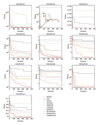
The stability analysis through boxplots in Figure 13 reveals that MCOA generates no outliers on CEC2019-01, CEC2019-02, and CEC2019-09, indicating excellent robustness. On CEC2019-05, the overall distribution of mean, maximum, and minimum values for MCOA is more concentrated than comparison algorithms. For CEC2019-03, CEC2019-04, CEC2019-07, and CEC2019-10, like the other methods, MCOA inevitably produced some outliers (+), which demonstrates that there is room for further improvement in the stability of MCOA. Generally, MCOA obtains more valuable interpretations and narrower box plots than other improved algorithms on most test functions.
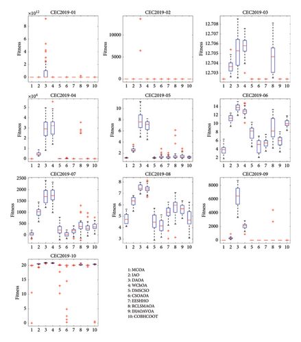
Table 12 presents the average computation time for 30 runs of each algorithm on the CEC2019 functions. It can be found that DAOA requires the least computational consumption, whereas our proposed MCOA is ranked fourth to last. Due to the introduction of several improvement strategies in MCOA, the optimization performance is improved at the expense of additional computational costs. On the whole, by taking some computational time in exchange for superior convergence accuracy, robustness, and local optimum avoidance, MCOA is acceptable, which coincides with the NFL theorem.
| Function | MCOA | IAO | DAOA | WChOA | DMSCSO | CSOAOA | EESHHO | RCLSMAOA | IHAOAVOA | COBHCOOT |
|---|---|---|---|---|---|---|---|---|---|---|
| CEC2019-01 | 0.8974 | 0.4329 | 0.1967 | 0.7003 | 0.6507 | 0.3770 | 0.1986 | 0.8030 | 0.4326 | 0.4496 |
| CEC2019-02 | 0.2837 | 0.1141 | 0.0533 | 0.5789 | 0.4388 | 0.0998 | 0.0591 | 0.3290 | 0.1612 | 0.1652 |
| CEC2019-03 | 0.1900 | 0.0923 | 0.0524 | 0.5861 | 0.4743 | 0.0842 | 0.0529 | 0.2825 | 0.1206 | 0.1232 |
| CEC2019-04 | 0.2540 | 0.1095 | 0.0541 | 0.3653 | 0.2839 | 0.1021 | 0.0524 | 0.2599 | 0.1361 | 0.1302 |
| CEC2019-05 | 0.1861 | 0.0943 | 0.0459 | 0.3674 | 0.2912 | 0.0981 | 0.0523 | 0.2624 | 0.1332 | 0.1108 |
| CEC2019-06 | 1.4323 | 0.9400 | 0.4843 | 0.8326 | 1.4418 | 1.4073 | 0.4832 | 3.0530 | 1.5969 | 1.0859 |
| CEC2019-07 | 0.1729 | 0.0911 | 0.0522 | 0.3501 | 0.2985 | 0.1124 | 0.0559 | 0.2813 | 0.1332 | 0.1029 |
| CEC2019-08 | 0.1734 | 0.0889 | 0.0424 | 0.3551 | 0.2994 | 0.1008 | 0.0566 | 0.2802 | 0.1261 | 0.0987 |
| CEC2019-09 | 0.1650 | 0.0802 | 0.0422 | 0.3620 | 0.2829 | 0.0907 | 0.0493 | 0.2403 | 0.1158 | 0.0989 |
| CEC2019-10 | 0.1808 | 0.0808 | 0.0411 | 0.3346 | 0.2977 | 0.1026 | 0.0534 | 0.2702 | 0.1362 | 0.1051 |
| Total runtime | 3.9356 | 2.1242 | 1.0647 | 4.8323 | 4.7591 | 2.5751 | 1.1134 | 6.0618 | 3.0919 | 2.4705 |
- Note: The best results obtained are highlighted in bold.
5.4. Comparison With Some Improved Peers on CEC2022 Functions
The IEEE CEC2022 test set contains 12 benchmark functions: unimodal, multimodal, hybrid, and composition. The search domains of these functions are more challenging and closer to real-world optimization problems than the previous benchmark problems. In the following, we will apply MCOA and the nine improved methods mentioned above to solve the CEC2022 benchmark functions. Table 13 summarizes the statistical results of each algorithm derived from 30 independent runs on the CEC2022 benchmark suite.
| Function | Metrics | MCOA | IAO | DAOA | WChOA | DMSCSO | CSOAOA | EESHHO | RCLSMAOA | IHAOAVOA | COBHCOOT |
|---|---|---|---|---|---|---|---|---|---|---|---|
| CEC2022-01 | Mean | 5.4619E + 02 | 7.0153E + 03 | 2.0583E + 05 | 1.9711E + 04 | 5.6561E + 03 | 1.4213E + 03 | 5.8385E + 02 | 2.1356E + 03 | 4.7250E + 02 | 3.1160E + 02 |
| Std | 7.2414E + 02 | 4.7663E + 03 | 7.3674E + 05 | 3.3409E + 04 | 1.8002E + 03 | 8.4268E + 02 | 5.1018E + 02 | 1.0036E + 04 | 1.7303E + 02 | 1.2314E + 01 | |
| p value | — | 4.1191E − 01 | 3.0199E − 11 | 8.9934E − 11 | 7.3891E − 11 | 8.1527E − 11 | 3.0199E − 11 | 5.5727E − 10 | 3.0199E − 11 | 3.0199E − 11 | |
| Rank | 3 | 8 | 10 | 9 | 7 | 5 | 4 | 6 | 2 | 1 | |
| CEC2022-02 | Mean | 4.0130E + 02 | 5.3125E + 02 | 4.1833E + 03 | 3.4114E + 03 | 4.1537E + 02 | 4.0510E + 02 | 4.2019E + 02 | 5.4172E + 02 | 4.1817E + 02 | 4.1190E + 02 |
| Std | 2.3691E + 00 | 8.0177E + 01 | 1.7246E + 03 | 1.4140E + 03 | 2.4052E + 01 | 1.7000E + 01 | 2.8388E + 01 | 4.9292E + 02 | 2.5833E + 01 | 1.9692E + 01 | |
| p value | — | 3.0199E − 11 | 3.0199E − 11 | 3.0199E − 11 | 1.1747E − 04 | 5.2978E − 01 | 2.3885E − 04 | 8.8910E − 10 | 2.2539E − 04 | 1.4918E − 06 | |
| Rank | 1 | 7 | 10 | 9 | 4 | 2 | 6 | 8 | 5 | 3 | |
| CEC2022-03 | Mean | 6.0161E + 02 | 6.3367E + 02 | 7.0167E + 02 | 6.8098E + 02 | 6.0519E + 02 | 6.0195E + 02 | 6.0835E + 02 | 6.0577E + 02 | 6.2682E + 02 | 6.0182E + 02 |
| Std | 7.3082E − 01 | 7.1698E + 00 | 1.7149E + 01 | 5.7724E + 00 | 3.5932E + 00 | 8.8014E + 00 | 7.8021E + 00 | 1.9555E + 01 | 1.2272E + 01 | 2.0253E + 00 | |
| p value | — | 3.0199E − 11 | 3.0199E − 11 | 3.0199E − 11 | 2.3768E − 07 | 7.1186E − 09 | 2.5974E − 05 | 1.9963E − 05 | 3.0199E − 11 | 3.3285E − 01 | |
| Rank | 1 | 8 | 10 | 9 | 4 | 3 | 6 | 5 | 7 | 2 | |
| CEC2022-04 | Mean | 8.1427E + 02 | 8.5159E + 02 | 9.2108E + 02 | 8.7534E + 02 | 8.2176E + 02 | 8.2446E + 02 | 8.2507E + 02 | 8.3266E + 02 | 8.2892E + 02 | 8.1350E + 02 |
| Std | 6.2931E + 00 | 7.2841E + 00 | 1.1218E + 01 | 7.1431E + 00 | 7.1065E + 00 | 7.2637E + 00 | 7.6197E + 00 | 1.7502E + 01 | 8.4220E + 00 | 5.1197E + 00 | |
| p value | — | 3.0199E − 11 | 3.0199E − 11 | 3.0199E − 11 | 9.7917E − 05 | 5.8587E − 06 | 2.3168E − 06 | 6.0459E − 07 | 2.6015E − 08 | 7.5059E − 01 | |
| Rank | 2 | 8 | 10 | 9 | 3 | 4 | 5 | 7 | 6 | 1 | |
| CEC2022-05 | Mean | 9.0003E + 02 | 1.1683E + 03 | 4.3285E + 03 | 2.0272E + 03 | 9.5169E + 02 | 1.1206E + 03 | 1.1514E + 03 | 1.2284E + 03 | 1.2971E + 03 | 9.0081E + 02 |
| Std | 1.0158E − 01 | 1.8490E + 02 | 1.0461E + 03 | 1.9073E + 02 | 4.1089E + 01 | 1.6228E + 02 | 1.5989E + 02 | 8.7634E + 02 | 1.7137E + 02 | 1.0143E + 00 | |
| p value | — | 3.0199E − 11 | 2.9991E − 11 | 3.0199E − 11 | 3.3384E − 11 | 3.0199E − 11 | 3.0199E − 11 | 3.6897E − 11 | 3.0199E − 11 | 9.7555E − 10 | |
| Rank | 1 | 6 | 10 | 9 | 3 | 4 | 5 | 7 | 8 | 2 | |
| CEC2022-06 | Mean | 2.7432E + 03 | 9.5348E + 06 | 1.7124E + 09 | 6.1105E + 08 | 4.1618E + 03 | 3.2472E + 03 | 3.5592E + 03 | 8.9260E + 06 | 3.7268E + 03 | 5.8353E + 03 |
| Std | 7.6254E + 02 | 8.7967E + 06 | 1.2258E + 09 | 4.4254E + 08 | 2.1189E + 03 | 1.3498E + 03 | 1.9222E + 03 | 3.8615E + 07 | 1.6828E + 03 | 6.4003E + 03 | |
| p value | — | 3.0199E − 11 | 3.0199E − 11 | 3.0199E − 11 | 6.7869E − 02 | 5.0114E − 01 | 6.1001E − 01 | 2.7548E − 03 | 5.5546E − 02 | 5.5611E − 04 | |
| Rank | 1 | 8 | 10 | 9 | 5 | 2 | 3 | 7 | 4 | 6 | |
| CEC2022-07 | Mean | 2.2174E + 03 | 2.0814E + 03 | 2.2618E + 03 | 2.2528E + 03 | 2.0329E + 03 | 2.0222E + 03 | 2.0269E + 03 | 2.0362E + 03 | 2.0580E + 03 | 2.0299E + 03 |
| Std | 5.0147E + 00 | 1.2905E + 01 | 5.8495E + 01 | 7.1837E + 01 | 1.0226E + 01 | 1.4310E + 01 | 1.6216E + 01 | 2.2348E + 01 | 3.0551E + 01 | 9.8930E + 00 | |
| p value | — | 3.0199E − 11 | 3.0199E − 11 | 3.0199E − 11 | 6.5277E − 08 | 1.1536E − 02 | 1.0576E − 03 | 2.8790E − 06 | 4.1997E − 10 | 6.5261E − 07 | |
| Rank | 1 | 8 | 10 | 9 | 5 | 2 | 3 | 6 | 7 | 4 | |
| CEC2022-08 | Mean | 2.2181E + 03 | 2.2410E + 03 | 4.7021E + 03 | 4.1903E + 03 | 2.2223E + 03 | 2.2185E + 03 | 2.2202E + 03 | 2.2534E + 03 | 2.2264E + 03 | 2.2249E + 03 |
| Std | 2.7113E + 00 | 5.9518E + 00 | 5.3602E + 03 | 8.3183E + 03 | 3.3018E + 00 | 6.1266E + 00 | 5.3535E + 00 | 5.1941E + 01 | 3.7604E + 00 | 5.2226E + 00 | |
| p value | — | 3.0199E − 11 | 3.0199E − 11 | 3.0199E − 11 | 5.2650E − 05 | 1.6238E − 01 | 9.3519E − 01 | 6.7220E − 10 | 2.3715E − 10 | 1.4733E − 07 | |
| Rank | 1 | 7 | 10 | 9 | 4 | 2 | 3 | 8 | 6 | 5 | |
| CEC2022-09 | Mean | 2.5293E + 03 | 2.6600E + 03 | 3.1096E + 03 | 3.2560E + 03 | 2.5379E + 03 | 2.5314E + 03 | 2.5348E + 03 | 2.5954E + 03 | 2.5406E + 03 | 2.5293E + 03 |
| Std | 4.0855E − 02 | 3.8420E + 01 | 2.4863E + 02 | 2.4635E + 02 | 2.8251E + 01 | 3.4716E + 00 | 1.1247E + 01 | 1.0729E + 02 | 1.3815E + 01 | 3.2935E − 02 | |
| p value | — | 3.0199E − 11 | 3.0199E − 11 | 3.0199E − 11 | 3.1830E − 01 | 1.7666E − 03 | 3.0339E − 03 | 3.0199E − 11 | 1.5638E − 02 | 5.0120E − 03 | |
| Rank | 2 | 8 | 9 | 10 | 5 | 3 | 4 | 7 | 6 | 1 | |
| CEC2022-10 | Mean | 2.5037E + 03 | 2.5713E + 03 | 3.5873E + 03 | 3.8978E + 03 | 2.5384E + 03 | 2.5507E + 03 | 2.5711E + 03 | 2.6300E + 03 | 2.5638E + 03 | 2.5379E + 03 |
| Std | 1.8250E + 01 | 8.1884E + 01 | 8.5524E + 02 | 8.4885E + 02 | 5.8853E + 01 | 6.3005E + 01 | 6.3079E + 01 | 1.9545E + 02 | 6.4392E + 01 | 5.4042E + 01 | |
| p value | — | 7.0430E − 07 | 4.1997E − 10 | 1.7769E − 10 | 2.3885E − 04 | 2.2658E − 03 | 4.1178E − 06 | 1.4918E − 06 | 1.1567E − 07 | 8.3026E − 01 | |
| Rank | 1 | 7 | 9 | 10 | 3 | 4 | 6 | 8 | 5 | 2 | |
| CEC2022-11 | Mean | 2.6003E + 03 | 2.8478E + 03 | 4.7517E + 03 | 4.4270E + 03 | 2.6659E + 03 | 2.6354E + 03 | 2.7828E + 03 | 2.8801E + 03 | 2.7056E + 03 | 2.6788E + 03 |
| Std | 1.8480E − 01 | 8.6038E + 01 | 7.5824E + 02 | 3.5935E + 02 | 1.0495E + 02 | 1.0284E + 02 | 1.9962E + 02 | 6.1461E + 02 | 1.8242E + 02 | 1.5665E + 02 | |
| p value | — | 6.0104E − 08 | 3.0199E − 11 | 3.0199E − 11 | 2.9727E − 01 | 2.5721E − 07 | 6.8432E − 01 | 2.6243E − 03 | 8.5000E − 02 | 3.9648E − 08 | |
| Rank | 1 | 7 | 10 | 9 | 3 | 2 | 6 | 8 | 5 | 4 | |
| CEC2022-12 | Mean | 2.8622E + 03 | 2.8739E + 03 | 3.1984E + 03 | 3.2648E + 03 | 2.8684E + 03 | 2.8673E + 03 | 2.8773E + 03 | 2.8766E + 03 | 2.8718E + 03 | 2.8641E + 03 |
| Std | 1.2103E + 00 | 2.5682E + 00 | 1.2713E + 02 | 1.4063E + 02 | 6.5321E + 00 | 6.5020E + 00 | 1.5807E + 01 | 1.9451E + 01 | 1.0634E + 01 | 1.5020E + 00 | |
| p value | — | 3.0199E − 11 | 3.0199E − 11 | 3.0199E − 11 | 1.4643E − 10 | 3.5201E − 07 | 3.0199E − 11 | 9.9186E − 11 | 1.8567E − 09 | 1.6062E − 06 | |
| Rank | 1 | 6 | 9 | 10 | 4 | 3 | 8 | 7 | 5 | 2 | |
| +/−/= | — | 11/1/0 | 12/0/0 | 12/0/0 | 9/3/0 | 9/3/0 | 9/3/0 | 12/0/0 | 11/1/0 | 10/2/0 | |
| Mean rank | 1.3333 | 7.3333 | 9.7500 | 9.2500 | 4.1667 | 3.0000 | 4.9167 | 7.0000 | 5.5000 | 2.7500 | |
| Final ranking | 1 | 8 | 10 | 9 | 4 | 3 | 5 | 7 | 6 | 2 | |
- Note: The best results obtained are highlighted in bold.
As can be seen in Table 13, MCOA achieves the optimal results on 9 out of 12 CEC2022 functions, including CEC2022-02, CEC2022-03, CEC2022-05, CEC2022-06, CEC2022-07, CEC2022-08, CEC2022-10, CEC2022-11, and CEC2022-12, whereas COBHCOOT provides the best performance on the remaining functions. In most multimodal, hybrid, and composite test cases, the convergence accuracy and stability of MCOA are more reliable than those of other comparison algorithms. On CEC2022-04 and CEC2022-09, MCOA is slightly behind COBHCOOT in second place, but the outcomes of both are still very close. This demonstrates that the expanded exploration strategy, specular reflection learning, and vertical crossover operator comprehensively enhance the exploration and local optimal avoidance ability of MCOA. From a statistical standpoint, MCOA significantly outperforms IAO on 11 problems, DAOA on 12 problems, WChOA on 12 problems, DMSCSO on 9 problems, CSOAOA on 9 problems, EESHHO on 9 problems, RCLSMAOA on 12 problems, IHAOAVOA on 11 problems, and COBHCOOT on 10 issues. The Friedman test results show that MCOA receives the best average ranking of 1.3333, followed by COBHCOOT and CSOAOA. MCOA can satisfactorily address highly intricate numerical optimization challenges.
Figure 14 shows the convergence curves of MCOA and competing algorithms on CEC2022 functions. MCOA can fulfill a smooth transition between exploration and exploitation in the initial stage of iteration on most test functions, and the final convergence accuracy is effectively guaranteed. These features are particularly demonstrated on CEC2022-03 and CEC2022-04. In contrast, algorithms such as DAOA and WChOA often exhibit poor solution accuracy due to their weak local optimal avoidance, which makes it difficult to explore the complex search domain in depth. These convergence patterns reaffirm the competitive advantage of MCOA in both convergence speed and accuracy.
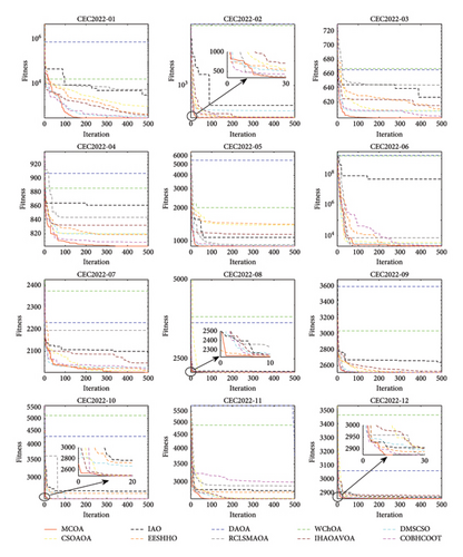
Figure 15 illustrates the boxplots of different algorithms on the IEEE CEC2022 test suite. MCOA generates no outliers on CEC2022-01, CEC2022-06, CEC2022-11, and CEC2022-12, and the data results are highly consistent. For the remaining test problems, MCOA also yields a few outliers, but compared to peer algorithms, its boxplots are narrower and the median, maximum, and minimum values are more concentrated. Compared to the CEC2019 experimental results, the performance of MCOA on the CEC2022 benchmark set is more impressive. Consequently, our proposed method can be expected to maintain good robustness even when confronted with more difficult numerical optimization issues.
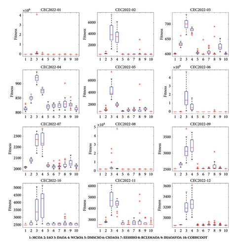
Table 14 presents the average computation time for each algorithm on the CEC2022 functions. The algorithms rank as follows in terms of computational efficiency: DAOA < EESHHO < IAO < COBHCOOT < CSOAOA < IHAOAVOA < MCOA < DSMSCSO < RCLSMAOA < WChOA. There is no doubt that DAOA wins by virtue of requiring the least amount of runtime, but its numerical optimization performance still needs to improve. Taking the above statistical results together, the advantages and limitations of MCOA are acceptable. While consuming slightly more computational time, MCOA provides high-quality and reliable solutions. With the continued advancement of cloud computing, distributed computing, and big data technologies, the computational requirements of MCOA have become increasingly feasible, making it particularly well-suited for intelligent optimization applications where high accuracy is paramount.
| Function | MCOA | IAO | DAOA | WChOA | DMSCSO | CSOAOA | EESHHO | RCLSMAOA | IHAOAVOA | COBHCOOT |
|---|---|---|---|---|---|---|---|---|---|---|
| CEC2022-01 | 0.5126 | 0.3261 | 0.1456 | 1.2956 | 0.6575 | 0.2535 | 0.2172 | 0.7032 | 0.3562 | 0.3320 |
| CEC2022-02 | 0.2629 | 0.1038 | 0.0432 | 0.4081 | 0.3114 | 0.1143 | 0.0584 | 0.2750 | 0.1585 | 0.1559 |
| CEC2022-03 | 0.2690 | 0.1183 | 0.0518 | 0.3819 | 0.3332 | 0.1617 | 0.0723 | 0.3462 | 0.1798 | 0.1729 |
| CEC2022-04 | 0.2405 | 0.1185 | 0.0493 | 0.4124 | 0.3100 | 0.1072 | 0.0506 | 0.2833 | 0.1664 | 0.1535 |
| CEC2022-05 | 0.1910 | 0.0893 | 0.0396 | 0.3535 | 0.2896 | 0.1129 | 0.0556 | 0.3051 | 0.1563 | 0.1431 |
| CEC2022-06 | 0.2255 | 0.1171 | 0.0488 | 0.4670 | 0.3720 | 0.1213 | 0.0637 | 0.3093 | 0.1664 | 0.1550 |
| CEC2022-07 | 0.2801 | 0.1454 | 0.0687 | 0.4384 | 0.3977 | 0.2183 | 0.0927 | 0.5195 | 0.2310 | 0.1682 |
| CEC2022-08 | 0.3301 | 0.1670 | 0.0760 | 0.4213 | 0.4280 | 0.2447 | 0.1048 | 0.5867 | 0.2875 | 0.1980 |
| CEC2022-09 | 0.2780 | 0.1385 | 0.0634 | 0.4319 | 0.3816 | 0.1862 | 0.0880 | 0.4773 | 0.2243 | 0.1732 |
| CEC2022-10 | 0.2588 | 0.1281 | 0.0628 | 0.4172 | 0.3797 | 0.1696 | 0.0781 | 0.3995 | 0.1948 | 0.1471 |
| CEC2022-11 | 0.3448 | 0.1660 | 0.0808 | 0.4845 | 0.4766 | 0.2719 | 0.1098 | 0.5704 | 0.2817 | 0.2020 |
| CEC2022-12 | 0.3580 | 0.1895 | 0.0950 | 0.5000 | 0.5089 | 0.3042 | 0.1219 | 0.6051 | 0.2879 | 0.2033 |
| Total runtime | 3.5513 | 1.8076 | 0.8251 | 6.0119 | 4.8463 | 2.2658 | 1.1130 | 5.3807 | 2.6907 | 2.2042 |
- Note: The best results obtained are highlighted in bold.
5.5. Summary of CEC Benchmark Experiments
- •
When the scale factor αF = 0.06, the Lévy flight strategy can more sufficiently strengthen the local search efficiency of MCOA and help circumvent local optima.
- •
For the 23 classic benchmark functions, MCOA provides the optimal solutions on 21 of them. As dimensionality increases, MCOA performs best on 12 out of 13 variable-dimensional benchmark functions in 50 dimensions, 12 out of 13 in 100 dimensions, 12 out of 13 in 500 dimensions, and 11 out of 13 in 1000 dimensions. On the CEC2019 test set, MCOA achieves the best convergence accuracy on 4 out of 10 functions. And on the CEC2022 test set, MCOA obtains the optimal average fitness results on 9 out of 12 functions.
- •
Compared to the original COA, the Wilcoxon rank-sum test and the Friedman ranking test suggest that MCOA exhibits significant enhancements in both exploration and exploitation capabilities. Through convergence curves and boxplot analysis, we confirm that MCOA possesses better convergence patterns and robustness than state-of-the-art improved methods such as DAOA, WChOA, DMSCSO, CSOAOA, EESHHO, RCLSMAOA, IHAOAVOA, and COBHCOOT.
The reasons behind these results can be understood from the ablation analysis in Section 5.2.3. Each improvement strategy enhances the algorithm’s search capabilities to some extent. The specular reflection learning enriches population diversity, the expanded exploration strategy boosts exploration trends, and the Lévy flight and vertical crossover operator enable MCOA to achieve more efficient local exploration and better local optima avoidance. The collaborative operation of these strategies achieves a more robust exploration–exploitation balance. Of course, according to the NFL theorem, no single algorithm can solve all optimization problems. Therefore, there is still room for improvement in the numerical results of MCOA on certain functions. However, in terms of overall performance, the proposed method significantly outperforms the comparison algorithms.
6. MCOA for Real-World Optimization Challenges
In this section, we evaluate the applicability of the proposed MCOA in solving two types of real-world optimization challenges: constrained engineering design and UAV path planning under complex terrain.
Constrained engineering design problems represent significant optimization challenges characterized by multiple design variables subject to various constraints. These problems require finding optimal designs that minimize objectives like cost or weight while meeting performance requirements and physical limitations. The complexity arises from nonlinear objective functions, intricate constraint interactions, and discontinuous search spaces. Our selected engineering design cases span mechanical and structural engineering domains. Traditional gradient-based methods often struggle with these problems due to their vulnerability to local optima and sensitivity to initial conditions.
UAV path planning involves determining optimal flight trajectories while balancing multiple conflicting objectives under various constraints. This task is particularly challenging due to several factors: UAVs must navigate three-dimensional environments while minimizing energy usage, flight time, and risk; they must avoid various obstacles including buildings, terrain features, and restricted airspace; they are constrained by physical limitations such as turning radius, climb rate, and velocity bounds; and they must account for environmental uncertainties like wind conditions. By applying MCOA to these complex path planning scenarios, we aim to demonstrate its ability to effectively balance exploration and exploitation while producing safe, efficient flight paths, thereby validating the algorithm’s practical effectiveness in solving real-world optimization challenges.
6.1. Constrained Engineering Design Cases
The maximum iterations and population size for each algorithm are fixed at 500 and 30, respectively, with other parameter settings aligning with the numerical experiments. Seven nonlinear engineering design cases with constraints are to be settled, including tension/compression spring design, three-bar truss design, I-beam design, welded beam design, tubular column design, cantilever beam design, and piston lever design. The optimal outcomes derived from 30 independent runs for each scenario are documented in the subsequent subsections.
6.1.1. Case 1: Tension/Compression Spring Design
The objective of this design optimization case is to minimize the weight of a tension/compression spring while adhering to constraints related to the outer diameter, deflection, shear stress, and surge frequency, as illustrated in Figure 16. This problem contains three decision variables to be optimized, namely: wire diameter d(z1), average coil diameter D(z2), and the number of active coils N(z3), which are mathematically described in Appendix B.1.

Twelve well-regarded MH algorithms (AO, DO, SO, AOA, ARO, TSA, SMA, COA, WHO, LCA, RIME, and SCSO), as well as nine latest enhanced optimizers (IAO, DAOA, WChOA, DMSCSO, CSOAOA, EESHHO, RCLSMAOA, IHAOAVOA, and COBHCOOT), are employed in parallel with MCOA to solve this case. The optimal solution and corresponding fitness values are summarized in Table 15. Notably, the proposed MCOA gets the first place, followed by WHO and SCSO. When d, D, and N are set to 0.05167105, 0.35628458, and 11.31440584, respectively, the tension/compression spring attains the minimum weight .
| Algorithm | Variables | Minimum weight | Ranking | ||
|---|---|---|---|---|---|
| d(z1) | D(z2) | N(z3) | |||
| MCOA | 0.05167105 | 0.35628458 | 11.31440584 | 0.01266524 | 1 |
| AO | 0.05000000 | 0.31595975 | 15.00000000 | 0.01342829 | 22 |
| DO | 0.05133183 | 0.34818407 | 11.80739683 | 0.01266759 | 9 |
| SO | 0.05186491 | 0.36096301 | 11.04435110 | 0.01266580 | 4 |
| AOA | 0.05000000 | 0.31049611 | 15.00000000 | 0.01319608 | 20 |
| ARO | 0.05157676 | 0.35400927 | 11.45355090 | 0.01266950 | 10 |
| TSA | 0.05000000 | 0.31532124 | 14.40123918 | 0.01292915 | 19 |
| SMA | 0.05137080 | 0.34910910 | 11.74939627 | 0.01266711 | 8 |
| COA | 0.05147564 | 0.35151492 | 11.61113327 | 0.01267773 | 13 |
| WHO | 0.05161011 | 0.35482133 | 11.40101877 | 0.01266535 | 2 |
| LCA | 0.05122637 | 0.34566146 | 11.97493341 | 0.01267617 | 12 |
| RIME | 0.05135404 | 0.34827829 | 11.82414583 | 0.01269737 | 16 |
| SCSO | 0.05178942 | 0.35913701 | 11.14855524 | 0.01266544 | 3 |
| IAO | 0.05035335 | 0.32531706 | 13.53811473 | 0.01281628 | 18 |
| DAOA | 0.05000000 | 0.31066615 | 15.00000000 | 0.01320331 | 21 |
| WChOA | 0.05196913 | 0.36349280 | 10.90257816 | 0.01266669 | 7 |
| DMSCSO | 0.05143710 | 0.35068643 | 11.65155381 | 0.01266642 | 6 |
| CSOAOA | 0.05142417 | 0.35028906 | 11.69044107 | 0.01268173 | 15 |
| EESHHO | 0.05246541 | 0.37568373 | 10.25791202 | 0.01267608 | 11 |
| RCLSMAOA | 0.05348341 | 0.40144043 | 9.07920539 | 0.01272237 | 17 |
| IHAOAVOA | 0.05189182 | 0.36161528 | 11.00751058 | 0.01266598 | 5 |
| COBHCOOT | 0.16751103 | 0.78491026 | 14.60163778 | 0.01267903 | 14 |
- Note: The best results obtained are highlighted in bold.
6.1.2. Case 2: Three-Bar Truss Design
The three-bar truss design problem is a representative optimization challenge in civil engineering, aiming to determine the optimal cross-sectional areas A1(z1) and A2(z2) under stress constraints, with the objective of minimizing the weight of the truss. Figure 17 illustrates the geometric structure of the three-bar truss and its three design variables. The mathematical formulation is provided in Appendix B.2.
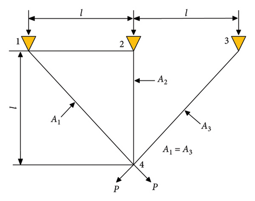
Table 16 reports the optimal variable values and minimum weight obtained by each algorithm. MCOA, WHO, and CSOAOA are tied for first place among all the methods since they achieve the same minimum weight of 263.89584338. This result underscores the significant potential of MCOA in addressing this design challenge.
| Algorithm | Variables | Minimum weight | Ranking | |
|---|---|---|---|---|
| A1(z1) | A2(z2) | |||
| MCOA | 0.78867718 | 0.40824250 | 263.89584338 | 1 |
| AO | 0.79295948 | 0.39673649 | 263.95646038 | 20 |
| DO | 0.78871402 | 0.40813840 | 263.89585293 | 8 |
| SO | 0.78868121 | 0.40823111 | 263.89584340 | 4 |
| AOA | 0.79417556 | 0.39322975 | 263.94974417 | 19 |
| ARO | 0.78866861 | 0.40826675 | 263.89584347 | 5 |
| TSA | 0.78276042 | 0.42544590 | 263.94267196 | 18 |
| SMA | 0.79283189 | 0.39895776 | 264.14249804 | 21 |
| COA | 0.78808321 | 0.40992669 | 263.89626240 | 13 |
| WHO | 0.78867512 | 0.40824833 | 263.89584338 | 1 |
| LCA | 0.78894134 | 0.40750072 | 263.89638119 | 14 |
| RIME | 0.78944190 | 0.40609388 | 263.89727480 | 15 |
| SCSO | 0.78914618 | 0.40691768 | 263.89601349 | 11 |
| IAO | 0.78833875 | 0.40921561 | 263.89743149 | 16 |
| DAOA | 0.79556463 | 0.40033693 | 265.05335225 | 22 |
| WChOA | 0.79398989 | 0.39341972 | 263.91622699 | 17 |
| DMSCSO | 0.78877971 | 0.40795259 | 263.89585141 | 7 |
| CSOAOA | 0.78867513 | 0.40824829 | 263.89584338 | 1 |
| EESHHO | 0.78873817 | 0.40807003 | 263.89584630 | 6 |
| RCLSMAOA | 0.78854867 | 0.40860612 | 263.89585514 | 9 |
| IHAOAVOA | 0.78846959 | 0.40882998 | 263.89587445 | 10 |
| COBHCOOT | 0.78923502 | 0.40666828 | 263.89621512 | 12 |
- Note: The best results obtained are highlighted in bold.
6.1.3. Case 3: I-Shaped Beam Design
This design problem aims to keep the vertical deflection of an I-shaped beam as low as possible without violating the conditions of the horizontal load (Q) and design load (P) acting at the midpoint of the span. As illustrated in Figure 18, flange width b(z1), section height h(z2), web thickness tw(z3), and flange thickness tf(z4) are the four critical design variables that need to be estimated in this case. The vertical deflection of the I-shaped beam is calculated using the formula PL3/(48EI), where L represents the length of the beam equal to 5200 cm and E denotes the elastic modulus of 523.104 kN/cm2. Mathematically, the design of an I-shaped beam is represented in Appendix B.3.
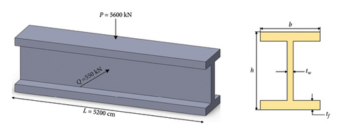
Table 17 shows the numerical results of I-shaped beam design optimization. MCOA and IHAOAVOA yield the same optimal weight , jointly ranking first among all the optimization methods. Hence, it is reasonable to conclude that MCOA is well-suited for effectively resolving this problem.
| Algorithm | Variables | Minimum fitness | Ranking | |||
|---|---|---|---|---|---|---|
| b (z1) | h (z2) | tw (z3) | tf (z4) | |||
| MCOA | 80.00000000 | 50.00000000 | 0.90000000 | 2.32179226 | 0.0130741189 | 1 |
| AO | 80.00000000 | 50.00000000 | 0.90000000 | 2.32173276 | 0.0130744025 | 11 |
| DO | 80.00000000 | 50.00000000 | 0.90000000 | 2.32179221 | 0.0130741191 | 3 |
| SO | 80.00000000 | 50.00000000 | 0.90000000 | 2.32178743 | 0.0130741419 | 8 |
| AOA | 80.00000000 | 50.00000000 | 0.90000000 | 2.32063163 | 0.0130796529 | 20 |
| ARO | 79.99956079 | 49.98710956 | 0.90003420 | 2.32234738 | 0.0130746747 | 13 |
| TSA | 80.00000000 | 50.00000000 | 0.90000000 | 2.32166970 | 0.0130747031 | 14 |
| SMA | 80.00000000 | 49.99998053 | 0.90000000 | 2.32179304 | 0.0130741199 | 5 |
| COA | 80.00000000 | 49.99996196 | 0.90000010 | 2.32179378 | 0.0130741206 | 6 |
| WHO | 80.00000000 | 50.00000000 | 0.90000000 | 2.32146225 | 0.0130756919 | 16 |
| LCA | 80.00000000 | 50.00000000 | 0.90000000 | 2.32178183 | 0.0130741686 | 9 |
| RIME | 80.00000000 | 50.00000000 | 0.90000000 | 2.32177680 | 0.0130741926 | 10 |
| SCSO | 80.00000000 | 49.75404110 | 0.90000000 | 2.33348132 | 0.0130776237 | 18 |
| IAO | 80.00000000 | 50.00000000 | 0.90000000 | 2.32035321 | 0.0130809812 | 21 |
| DAOA | 80.00000000 | 50.00000000 | 0.90000000 | 2.31982154 | 0.0130835184 | 22 |
| WChOA | 80.00000000 | 50.00000000 | 0.90000000 | 2.32179216 | 0.0130741194 | 4 |
| DMSCSO | 79.99888209 | 49.96502190 | 0.90000266 | 2.32345566 | 0.0130749661 | 15 |
| CSOAOA | 80.00000000 | 50.00000000 | 0.90000000 | 2.32114115 | 0.0130772228 | 17 |
| EESHHO | 80.00000000 | 50.00000000 | 0.90017691 | 2.32165611 | 0.0130745521 | 12 |
| RCLSMAOA | 80.00000000 | 49.98296942 | 0.90166652 | 2.32131856 | 0.0130784250 | 19 |
| IHAOAVOA | 80.00000000 | 50.00000000 | 0.90000000 | 2.32179226 | 0.0130741189 | 1 |
| COBHCOOT | 80.00000000 | 40.97785551 | 1.48603832 | 1.82250020 | 0.0130741217 | 7 |
- Note: The best results obtained are highlighted in bold.
6.1.4. Case 4: Welded Beam Design
The purpose of the welded beam design challenge is to minimize the fabrication cost of a welded beam subject to the constraints on shear stress τ, buckling load Pc, bending stress θ, and end deflection δ. As depicted in Figure 19, four design variables require optimization: the weld width h(z1), the length of clamped beam l(z2), the height of beam t(z3), and the thickness of beam b(z4). Its mathematical model is presented in Appendix B.4.
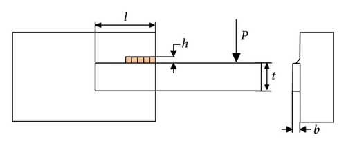
Table 18 presents the optimal solutions and the corresponding fitness values achieved by different algorithms for the welded beam design. According to the tabulated data, the proposed method provides a better outcome than the remaining competitor algorithms. The minimum fabrication cost of MCOA is 1.69276826 when the values of h, l, t, and b are fixed to 0.20572964, 3.23491931, 9.03662391, and 0.20572964, respectively. MCOA demonstrates a more pronounced advantage in welded beam design.
| Algorithm | Variables | Minimum cost | Ranking | |||
|---|---|---|---|---|---|---|
| h(z1) | l(z2) | t(z3) | b(z4) | |||
| MCOA | 0.20572964 | 3.23491931 | 9.03662391 | 0.20572964 | 1.69276826 | 1 |
| AO | 0.21243450 | 3.19396666 | 8.87672213 | 0.21627365 | 1.74729423 | 16 |
| DO | 0.20571591 | 3.23535159 | 9.03662766 | 0.20573020 | 1.69281177 | 3 |
| SO | 0.20575334 | 3.23467548 | 9.03611122 | 0.20575358 | 1.69286179 | 5 |
| AOA | 0.16808434 | 3.74244228 | 10.00000000 | 0.20157933 | 1.83746280 | 21 |
| ARO | 0.20573974 | 3.23491504 | 9.03648462 | 0.20574048 | 1.69283996 | 4 |
| TSA | 0.18457418 | 3.64640566 | 9.21662122 | 0.20659936 | 1.75379380 | 17 |
| SMA | 0.20565051 | 3.23681869 | 9.03671035 | 0.20572983 | 1.69292674 | 6 |
| COA | 0.20564335 | 3.23768156 | 9.03931468 | 0.20572985 | 1.69347815 | 7 |
| WHO | 0.20614114 | 3.23881826 | 9.02655447 | 0.20619428 | 1.69566604 | 12 |
| LCA | 0.20533297 | 3.24533696 | 9.03755601 | 0.20573492 | 1.69380127 | 9 |
| RIME | 0.19731885 | 3.42042334 | 9.03068700 | 0.20600764 | 1.70630471 | 14 |
| SCSO | 0.22165273 | 3.07754403 | 8.69532968 | 0.22690525 | 1.78806280 | 19 |
| IAO | 0.19909152 | 3.38305446 | 9.05196850 | 0.21222536 | 1.75471456 | 18 |
| DAOA | 0.13140212 | 6.04504374 | 9.32653815 | 0.23795146 | 2.25549059 | 22 |
| WChOA | 0.17532672 | 4.05852977 | 9.63981107 | 0.20290428 | 1.83714935 | 20 |
| DMSCSO | 0.20546452 | 3.23373175 | 9.05164428 | 0.20565482 | 1.69421763 | 11 |
| CSOAOA | 0.20572841 | 3.23494311 | 9.03664859 | 0.20572952 | 1.69277299 | 2 |
| EESHHO | 0.20527672 | 3.24579385 | 9.03318141 | 0.20588647 | 1.69416970 | 10 |
| RCLSMAOA | 0.19012164 | 3.66191333 | 9.00989425 | 0.20695213 | 1.73061646 | 15 |
| IHAOAVOA | 0.20335892 | 3.28334933 | 9.03899708 | 0.20571780 | 1.69616360 | 13 |
| COBHCOOT | 0.16686851 | 8.18455175 | 6.74641513 | 0.37202703 | 1.69375249 | 8 |
- Note: The best results obtained are highlighted in bold.
6.1.5. Case 5: Tubular Column Design
The tubular column optimization involves designing a uniform column with a tubular cross section to support an axial load P at minimum cost, as depicted in Figure 20. The column is constructed from a material with the elastic modulus of E = 0.85 × 10⁶ kgf/cm2 and the yield stress of σy = 500 kgf/cm2. In this problem, two optimal parameters need to be identified: the column’s mean diameter d(z1) and tube thickness t(z2). The mathematical model for this case can be found in Appendix B.5.
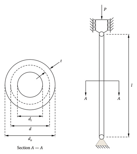
Table 19 presents a comparison of the optimal decision variables and the minimum cost acquired through MCOA and various optimization methodologies for this design scenario. MCOA, ARO, WHO, and CSOAOA are all ranked first, with a minimum fitness value of 26.48636147, proving the suggested optimizer’s favorable competition in solving the tubular column design. On the other hand, there are still some gaps between other comparison methods and MCOA regarding solution accuracy.
| Algorithm | Variables | Minimum cost | Ranking | |
|---|---|---|---|---|
| d(z1) | t(z2) | |||
| MCOA | 5.45218074 | 0.29162643 | 26.48636147 | 1 |
| AO | 5.44347115 | 0.29343537 | 26.54055044 | 20 |
| DO | 5.45218124 | 0.29162643 | 26.48636369 | 7 |
| SO | 5.45226239 | 0.29162743 | 26.48681171 | 12 |
| AOA | 5.53203767 | 0.29428059 | 27.01819425 | 21 |
| ARO | 5.45218074 | 0.29162643 | 26.48636147 | 1 |
| TSA | 5.44987539 | 0.29237177 | 26.51497022 | 19 |
| SMA | 5.45218741 | 0.29162625 | 26.48638448 | 9 |
| COA | 5.45219635 | 0.29162571 | 26.48639886 | 10 |
| WHO | 5.45218074 | 0.29162643 | 26.48636147 | 1 |
| LCA | 5.45240618 | 0.29163330 | 26.48782385 | 13 |
| RIME | 5.45635450 | 0.29142165 | 26.49568712 | 15 |
| SCSO | 5.46033217 | 0.29119111 | 26.50266612 | 17 |
| IAO | 5.44688475 | 0.29255452 | 26.51017508 | 18 |
| DAOA | 5.21392106 | 0.35658628 | 28.64812652 | 22 |
| WChOA | 5.44954872 | 0.29204599 | 26.49598222 | 16 |
| DMSCSO | 5.45218072 | 0.29162643 | 26.48636153 | 5 |
| CSOAOA | 5.45218074 | 0.29162643 | 26.48636147 | 1 |
| EESHHO | 5.45218252 | 0.29162633 | 26.48636504 | 8 |
| RCLSMAOA | 5.44963078 | 0.29203288 | 26.49568114 | 14 |
| IHAOAVOA | 5.45218035 | 0.29162650 | 26.48636347 | 6 |
| COBHCOOT | 4.95225730 | 0.47328918 | 26.48645977 | 11 |
- Note: The best results obtained are highlighted in bold.
6.1.6. Case 6: Cantilever Beam Design
This structural design case focuses on optimizing the total weight of a cantilever beam. The cantilever beam comprises five hollow elements with a square cross section, rigidly supported at the first element, whereas a given vertical force is applied at the fifth element, as illustrated in Figure 21. The width of each beam element zi(i = 1, 2, …, 5) represents a design variable, and the thickness is held constant. The mathematical definition of this problem is outlined in Append B.6.
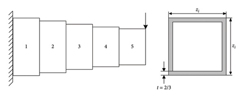
The values of the optimized decision variables and the minimum weight for each algorithm are recorded in Table 20. From the results, MCOA outperforms all other competitors as it reveals a minimum weight of 1.33995767. Thus, MCOA performs an excellent optimization effect in addressing this engineering issue.
| Algorithm | Variables | Minimum weight | Ranking | ||||
|---|---|---|---|---|---|---|---|
| z1 | z2 | z3 | z4 | z5 | |||
| MCOA | 6.01738279 | 5.31234147 | 4.48996478 | 3.50367197 | 2.15031959 | 1.33995767 | 1 |
| AO | 6.14811254 | 5.42142456 | 4.33757745 | 3.39423369 | 2.20855305 | 1.34221784 | 16 |
| DO | 6.01762482 | 5.30410695 | 4.52306027 | 3.50375732 | 2.12663244 | 1.34005134 | 9 |
| SO | 6.01972060 | 5.30356939 | 4.49369427 | 3.50737041 | 2.14943104 | 1.33996423 | 3 |
| AOA | 8.52009058 | 8.42615912 | 3.76122853 | 2.88700239 | 2.21182768 | 1.61031364 | 22 |
| ARO | 6.03756468 | 5.30432522 | 4.49047601 | 3.48947675 | 2.15208679 | 1.33997320 | 4 |
| TSA | 5.87753978 | 5.37888456 | 4.59208953 | 3.55140060 | 2.09503293 | 1.34128472 | 15 |
| SMA | 6.05850070 | 5.28268294 | 4.47962105 | 3.50631853 | 2.14800134 | 1.34004777 | 8 |
| COA | 6.00520946 | 5.32041324 | 4.48771156 | 3.49455178 | 2.16609664 | 1.33997652 | 5 |
| WHO | 6.02081916 | 5.31398285 | 4.48273285 | 3.50121199 | 2.15499432 | 1.33996145 | 2 |
| LCA | 6.02735882 | 5.29169389 | 4.50381919 | 3.49978367 | 2.15145657 | 1.33998460 | 7 |
| RIME | 5.74255302 | 5.48713349 | 4.77903079 | 3.37354957 | 2.17885297 | 1.34541388 | 17 |
| SCSO | 6.00614912 | 6.12385869 | 3.70253473 | 4.21419281 | 2.23571179 | 1.39042470 | 20 |
| IAO | 6.05733849 | 5.36905293 | 4.23904778 | 3.37690985 | 2.79266084 | 1.36250462 | 19 |
| DAOA | 8.86752494 | 4.47381323 | 3.71699050 | 5.22980815 | 2.47384114 | 1.54514742 | 21 |
| WChOA | 6.48005691 | 5.03920848 | 4.39817327 | 4.05385796 | 1.84866637 | 1.36156569 | 18 |
| DMSCSO | 5.95853366 | 5.20753982 | 4.56652756 | 3.50006980 | 2.25821669 | 1.34103138 | 13 |
| CSOAOA | 5.98703556 | 5.30867170 | 4.57331357 | 3.45516758 | 2.15370757 | 1.34022071 | 10 |
| EESHHO | 5.95126828 | 5.28559554 | 4.48479298 | 3.55423371 | 2.20328082 | 1.34030029 | 11 |
| RCLSMAOA | 6.00475844 | 5.28040681 | 4.37282991 | 3.63757109 | 2.19711311 | 1.34114319 | 14 |
| IHAOAVOA | 6.00811900 | 5.22698247 | 4.54671389 | 3.49683956 | 2.20094645 | 1.34032713 | 12 |
| COBHCOOT | 3.96524768 | 16.03706041 | 71.10635175 | 25.30585626 | 21.97619575 | 1.33997974 | 6 |
- Note: The best results obtained are highlighted in bold.
6.1.7. Case 7: Piston Lever Design
The last test case pertains to the design of a piston lever, wherein the ultimate target is to locate the optimal values of four design variables H(z1), B(z2), D(z3), X(z4) for different piston components so as to minimize the amount of oil required to lift the piston lever from 0° to 45°, as can be seen in Figure 22. This problem is mathematically formulated in Appendix B.7.
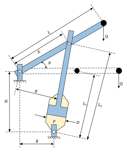
Table 21 summarizes the minimum cost and the four corresponding variables of MCOA and other comparative optimization methods. The tabulated data highlight MCOA as the most effective optimizer for tackling the piston lever design case, as it reveals the best design with the minimum cost . Based on these results, MCOA provides a superior solution for the piston lever design.
| Algorithm | Variables | Minimum cost | Ranking | |||
|---|---|---|---|---|---|---|
| H (z1) | B (z2) | D (z3) | X (z4) | |||
| MCOA | 0.05000000 | 2.04151359 | 4.08302718 | 120.00000000 | 8.41269832 | 1 |
| AO | 0.05000000 | 2.05385971 | 4.08495418 | 120.00000000 | 8.46947284 | 17 |
| DO | 0.05000000 | 2.04151401 | 4.08302754 | 120.00000000 | 8.41270148 | 4 |
| SO | 0.05000000 | 2.04206436 | 4.08361374 | 119.97886535 | 8.41731392 | 13 |
| AOA | 0.05000125 | 2.04157994 | 4.08313277 | 119.99853952 | 8.41340882 | 9 |
| ARO | 0.05004260 | 2.04156710 | 4.08308405 | 119.99666220 | 8.41354659 | 10 |
| TSA | 0.06142367 | 2.04851934 | 4.09004933 | 120.00000000 | 8.57681980 | 19 |
| SMA | 0.05000000 | 2.04151486 | 4.08302743 | 120.00000000 | 8.41270438 | 6 |
| COA | 0.05000191 | 2.04156497 | 4.08309059 | 120.00000000 | 8.41318056 | 8 |
| WHO | 0.05018272 | 2.04169729 | 4.08338120 | 120.00000000 | 8.41659517 | 12 |
| LCA | 0.05000000 | 2.04266768 | 4.08310044 | 120.00000000 | 8.41756041 | 14 |
| RIME | 0.05000000 | 2.04372194 | 4.08587671 | 120.00000000 | 8.43318265 | 16 |
| SCSO | 0.05000000 | 2.04508593 | 4.08338038 | 119.97515883 | 8.42829689 | 15 |
| IAO | 0.05000000 | 2.06943426 | 4.12557716 | 117.66672171 | 8.70414342 | 21 |
| DAOA | 0.05000000 | 2.25549892 | 4.49825596 | 98.24966930 | 11.27862081 | 22 |
| WChOA | 0.05000000 | 2.07931091 | 4.09393916 | 119.31009538 | 8.60864330 | 20 |
| DMSCSO | 0.05000061 | 2.04151404 | 4.08302808 | 119.99998870 | 8.41270958 | 7 |
| CSOAOA | 0.05000001 | 2.04151447 | 4.08302764 | 119.99999009 | 8.41270382 | 5 |
| EESHHO | 0.05000000 | 2.04151359 | 4.08302718 | 120.00000000 | 8.41269833 | 2 |
| RCLSMAOA | 0.05000000 | 2.08176791 | 4.08327557 | 119.94346366 | 8.57289798 | 18 |
| IHAOAVOA | 0.05000000 | 2.04151362 | 4.08302723 | 119.99999849 | 8.41269867 | 3 |
| COBHCOOT | 427.65773392 | 177.54973049 | 53.27476217 | 118.19214246 | 8.41493494 | 11 |
- Note: The best results obtained are highlighted in bold.
6.2. UAV Path Planning in Complex Terrain
The main objective of UAV path planning is to find an optimal path from the start position to the goal position with the lowest cost, no collision, and satisfying various metrics, including threat constraints, energy consumption, and path lengths. This can be regarded as a typical nondeterministic polynomial-time hard (NP-hard) optimization problem. Figure 23 illustrates the principal model of UAV path planning, where the hexagon and star represent the start and target points, respectively, and the circles represent the obstacles and threat regions to be averted. Connect the start and target points with an S-T line and divide the S-T line segment into k equal parts with k + 1 vertical lines (L1, L2, …, Lk, Lk+1). One discrete point is taken at each vertical component Lk to form a set of discrete point sets P = {Start, L1(x(1), y(1)), L2(x(2), y(2)), …, Lk(x(k), y(k)), Lk+1(x(k + 1), y(k + 1)), Target}, which are then joined to create a path.
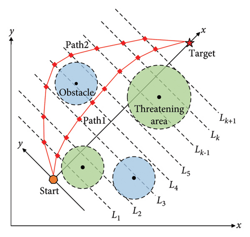
Traditional path planning methods such as A∗, Dijkstra, and rapidly exploring random tree frequently suffer from high time cost, slow convergence speed, and susceptibility to local optima, limiting their efficacy in solving path design problems with higher precision and flexibility requirements. Yet, the emergence of MH algorithms provides scholars with a brand-new idea. MH algorithm has good adaptive ability and strong global search performance, so generating effective paths in complex three-dimensional environments is possible [67]. This part employs MCOA and other comparison algorithms to address the UAV path planning problem and further investigate their competitiveness in complex optimization tasks.
6.2.1. Environment Model
In practical operations, the UAV must avoid no-fly zones, enemy radars, and surface-to-air missiles, among other potential threats. For simplicity, we use a cylinder of radius r to construct threat areas for the UAV to evade. We design two test cases. In the first test case, the flight area is 200 × 200 × 10 km. The second test case involves a more challenging scenario, with a larger flight area of 300 × 300 × 10 km. Based on the data specified in Table 22, the final three-dimensional environmental model for path planning incorporates terrain, mountains, and threat zones, as illustrated in Figure 24.
| No. | Peak | Center coordinate (km) | Altitude (km) | X slope | Y slope | Threat area | Center coordinate (km) | Radius (km) |
|---|---|---|---|---|---|---|---|---|
| Case 1 | Peak 1 | (50, 80) | 2 | 20 | 20 | Threat 1 | (40, 100) | 20 |
| Peak 2 | (70, 160) | 4 | 30 | 20 | Threat 2 | (90, 120) | 20 | |
| Peak 3 | (120, 40) | 4 | 30 | 20 | Threat 3 | (120, 60) | 20 | |
| Peak 4 | (160, 80) | 8 | 20 | 20 | ||||
| Peak 5 | (140, 140) | 6 | 20 | 20 | ||||
| Case 2 | Peak 1 | (60, 50) | 4 | 25 | 25 | Threat 1 | (40, 120) | 20 |
| Peak 2 | (60, 250) | 7 | 30 | 25 | Threat 2 | (140, 50) | 20 | |
| Peak 3 | (80, 160) | 5 | 18 | 20 | Threat 3 | (160, 250) | 20 | |
| Peak 4 | (150, 150) | 8 | 45 | 50 | Threat 4 | (260, 150) | 20 | |
| Peak 5 | (220, 80) | 4 | 35 | 40 | ||||
| Peak 6 | (240, 230) | 6 | 20 | 30 | ||||
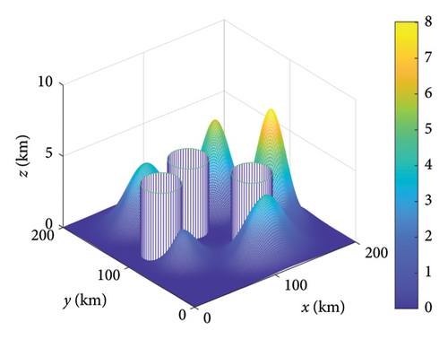
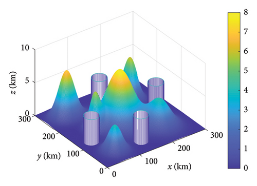
6.2.2. Cost Function
6.2.3. Experimental Results and Discussion
Case 1: Set the start coordinate position of the experimental flight as (0, 0, 0.5) and the target position as (200, 200, 1), with the number of path nodes n = 2. Case 2: Set the start coordinate position of the experimental flight as (0, 0, 1) and the target position as (300, 300, 3), with the number of path nodes n = 3. The maximum turning angle is 60°, and the weights ωi in the cost function are set to 0.4, 0.4, and 0.2, respectively. For MCOA and other comparison optimization methods, each algorithm operates independently for 30 runs with a population size of 30 and a maximum iteration number of 100. The generated paths are smoothed using a cubic B-spline curve [69].
6.2.3.1. Analysis of Case 1
The results presented in Table 23 reveal that MCOA provides the best path planning solution in complex 3D environments. The mean value obtained by MCOA is 134.6067, representing a 10.83% reduction compared to the original COA algorithm. Additionally, MCOA exhibits the smallest standard deviation, indicating superior robustness. Regarding optimal path cost, the proposed method achieves a value of 126.6594, ranking first among all algorithms, followed by COBHCOOT and IHAOAVOA.
| Algorithm | Mean | Std | Best | Ranking |
|---|---|---|---|---|
| MCOA | 134.6067 | 4.4420 | 126.6594 | 1 |
| AO | 143.4890 | 5.2160 | 136.2224 | 14 |
| DO | 153.7499 | 6.3422 | 144.4809 | 18 |
| SO | 154.1237 | 4.7674 | 146.0373 | 19 |
| AOA | 156.2093 | 7.9677 | 146.2621 | 20 |
| ARO | 140.5590 | 4.8006 | 132.8115 | 9 |
| TSA | 158.4664 | 8.8239 | 147.3131 | 21 |
| SMA | 145.1958 | 5.7585 | 135.4345 | 15 |
| COA | 150.9587 | 7.0876 | 139.2673 | 17 |
| WHO | 142.8026 | 5.6703 | 133.7797 | 13 |
| LCA | 158.7778 | 9.4366 | 144.6035 | 22 |
| RIME | 141.3434 | 5.7546 | 132.7490 | 12 |
| SCSO | 140.0591 | 5.7840 | 132.3410 | 8 |
| IAO | 140.9311 | 6.6127 | 131.6480 | 10 |
| DAOA | 145.4497 | 7.7425 | 135.1069 | 16 |
| WChOA | 141.1081 | 6.8013 | 131.1581 | 11 |
| DMSCSO | 138.0222 | 5.6192 | 128.4782 | 5 |
| CSOAOA | 137.9742 | 6.5247 | 127.0370 | 4 |
| EESHHO | 138.1802 | 4.7706 | 130.7490 | 6 |
| RCLSMAOA | 138.2561 | 6.8645 | 129.0225 | 7 |
| IHAOAVOA | 136.2638 | 5.6735 | 127.5238 | 2 |
| COBHCOOT | 136.5773 | 5.9118 | 126.7358 | 3 |
- Note: The best results obtained are highlighted in bold.
Figure 25 visualizes the performance of all algorithms in Case 1. The convergence curve in Figure 25(a) demonstrates that MCOA has a fast convergence speed and can locate the region where the global optimum may exist through less than 10 iterations. Enhanced by the specular reflection learning and vertical crossover operator, MCOA effectively escapes local optima and achieves the highest convergence accuracy. While DMSCSO and CSOAOA also show competitive convergence speeds, MCOA’s overall search performance is superior. The 3D view in Figure 25(b), X-Y plane top view in Figure 25(c), and side view in Figure 25(d) illustrate that MCOA successfully avoids all obstacles and threat areas while generating the shortest path. The algorithm’s ability to navigate efficiently through complex terrain demonstrates its superior decision-making capabilities in high-dimensional search spaces.
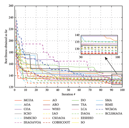
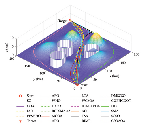
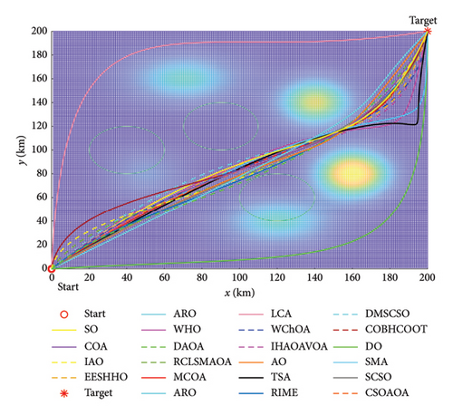
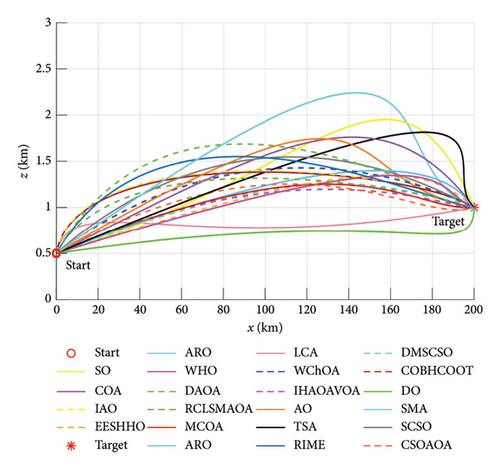
6.2.3.2. Analysis of Case 2
Table 24 presents the numerical results for the more challenging Case 2 scenario, which features longer distances and additional threat constraints. MCOA continues to demonstrate superior performance with a mean value of 236.9840, which represents a 7.61% improvement over the original COA algorithm (256.5099). Despite the increased problem complexity, MCOA maintains competitive robustness with a standard deviation of 14.3125. In terms of optimal path cost, MCOA again ranks first with a value of 217.3903, followed by IHAOAVOA (218.3255) and CSOAOA (218.4870). This consistent top-ranking performance across both test cases with different complexity levels confirms the effectiveness and adaptability of MCOA.
| Algorithm | Mean | Std | Best | Ranking |
|---|---|---|---|---|
| MCOA | 236.9840 | 14.3125 | 217.3903 | 1 |
| AO | 262.9066 | 16.4338 | 241.1270 | 19 |
| DO | 256.1609 | 16.4581 | 234.7058 | 12 |
| SO | 256.4368 | 18.4539 | 229.1236 | 10 |
| AOA | 259.0532 | 16.4648 | 240.8990 | 18 |
| ARO | 247.4527 | 14.8282 | 225.5775 | 6 |
| TSA | 289.6658 | 16.7635 | 267.1326 | 22 |
| SMA | 259.4073 | 14.3959 | 239.0314 | 16 |
| COA | 256.5099 | 13.4672 | 235.4826 | 14 |
| WHO | 259.9700 | 17.2747 | 236.7984 | 15 |
| LCA | 275.3463 | 16.1519 | 253.4875 | 20 |
| RIME | 258.3066 | 12.5638 | 234.7642 | 13 |
| SCSO | 262.7354 | 14.9530 | 239.6591 | 17 |
| IAO | 250.6219 | 15.8789 | 227.2110 | 7 |
| DAOA | 252.2951 | 16.0523 | 228.7370 | 9 |
| WChOA | 274.3636 | 15.2650 | 254.6457 | 21 |
| DMSCSO | 247.3743 | 12.0350 | 223.6382 | 5 |
| CSOAOA | 239.8799 | 16.1351 | 218.4870 | 3 |
| EESHHO | 254.0341 | 16.8257 | 230.4508 | 11 |
| RCLSMAOA | 256.1495 | 16.8055 | 228.0506 | 8 |
| IHAOAVOA | 240.7347 | 12.2784 | 218.3255 | 2 |
| COBHCOOT | 242.4634 | 15.1290 | 221.9067 | 4 |
- Note: The best results obtained are highlighted in bold.
The convergence curve in Figure 26(a) reveals that MCOA maintains its advantage in convergence speed even in this more challenging environment, reaching near-optimal solutions within approximately 60 iterations. While several algorithms show similar early convergence patterns, MCOA ultimately achieves superior final solutions through its enhanced balance between exploration and exploitation. The 3D visualization in Figure 26(b) clearly demonstrates that MCOA can efficiently navigate through complex terrain, avoiding all potential threats to cross the extended distance. The top view in Figure 26(c) and side view in Figure 26(d) further confirm MCOA’s ability to generate smooth, obstacle-avoiding paths that satisfy all constraints while minimizing the total path cost.
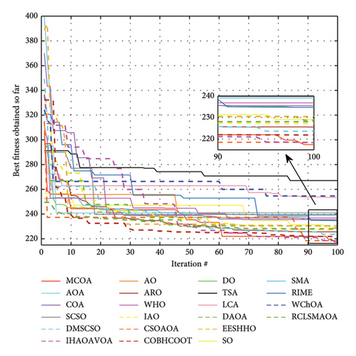
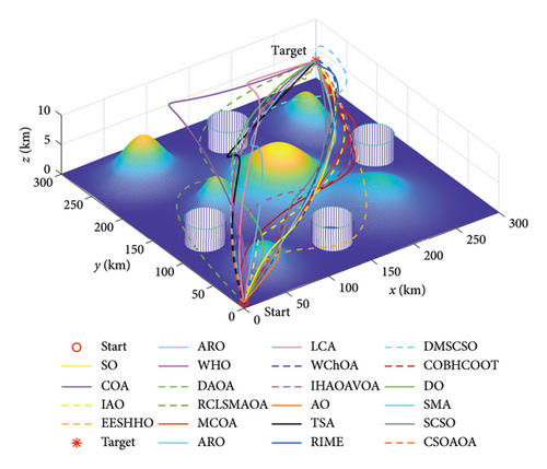
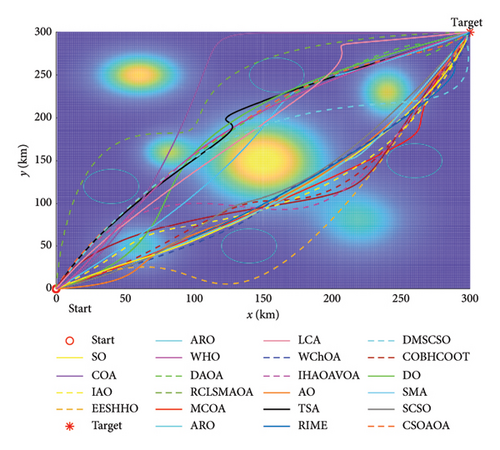
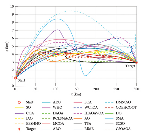
Specular reflection learning enhances population diversity, expanding the search space. The expanded exploration strategy boosts global search capabilities and accelerates convergence. Lévy flight increases local search efficiency, and the vertical crossover operator helps escape local optima. These strategies work synergistically to provide MCOA with superior exploration–exploitation balance, enabling it to outperform other algorithms in solving constrained engineering problems and UAV path planning, demonstrating its robustness and adaptability in complex optimization challenges.
7. Conclusion
This paper presents a multistrategy MCOA designed to address the limitations of the original algorithm, such as premature convergence, slow convergence speed, and an imbalance between exploration and exploitation. The proposed MCOA incorporates four innovative strategies: specular reflection learning, expanded exploration strategy, Lévy flight, and vertical crossover operator. The integration of these strategies creates several advantages. Specular reflection learning increases population diversity and establishes a strong foundation for global search in the early iterations, while the extended exploration model extracted from AO significantly enhances exploration capabilities. Additionally, Lévy flight characteristics replace the random step size in the exploitation phase for more efficient convergence toward the global optimum, and the vertical crossover operator effectively mitigates search stagnation, preventing the algorithm from being trapped in local optima. These enhancements enable MCOA to maintain robust optimization performance across a wide range of benchmark functions and practical engineering problems, including the CEC2005, CEC2019, and CEC2022 test suites, as well as seven constrained engineering design tasks and UAV path planning cases in a complex three-dimensional environment. The experimental results confirm that MCOA outperforms twelve state-of-the-art MH algorithms and nine recent variants in terms of solution precision, local optima avoidance, convergence speed, and scalability across different spatial scales. Notably, the vertical crossover operator has the most significant impact on improving optimization performance, and the optimal scale factor αF for Lévy flight is found to be 0.06. The findings from engineering design problems and UAV path planning further demonstrate MCOA’s competitive edge in real-world applications.
However, while MCOA shows promising results, there are areas for improvement. The incorporation of multiple strategies leads to higher time costs, which may limit its suitability for specific real-time applications. Future work could focus on reducing these time costs by restructuring MCOA in parallel. Additionally, an adaptive dynamic adjustment strategy for the scale factor αF can be developed based on the number of iterations, allowing MCOA to exhibit superior performance in more comprehensive benchmark functions and more challenging engineering scenarios. Moreover, MCOA has the potential to be applied to a broader range of emerging optimization problems, such as parameter identification of photovoltaic models, image segmentation, battery health state estimation, manufacturing schedule, and hyperparameter tuning of neural networks.
Conflicts of Interest
The authors declare no conflicts of interest.
Author Contributions
Yaning Xiao: software, methodology, conceptualization, writing – original draft, and writing – review and editing. Hao Cui: investigation, validation, writing – review and editing, and formal analysis. Ruba Abu Khurma: methodology, conceptualization, and writing – original draft. Abdelazim G. Hussien: methodology and writing – review and editing. Pedro A. Castillo: writing – original draft and funding.
Funding
This work was supported by the Ministerio Español de Ciencia e Innovación under project numbers PID2020-115570GB-C22 MCIN/AEI/10.13039/501100011033 and PID2023-147409NB-C21 MICIU/AEI/10.13039/501100011033, the C-ING-027-UGR23 Project, and the Cátedra de Empresa Tecnología Para las Personas (UGR-Fujitsu).
Supporting Information
Supporting Information consists of two parts: Appendix A “Benchmark function description” and Appendix B “Case study on engineering optimization.” In Appendix A, detailed descriptions are provided for unimodal benchmark functions, multimodal benchmark functions, fixed-dimension multimodal benchmark functions, the IEEE CEC2019 test suite, and the IEEE CEC2022 test suite. In Appendix B, mathematical models for constrained engineering optimization design cases are provided.
Open Research
Data Availability Statement
All data used to support the findings of this study are included in this published article.


