International Journal of Intelligent Systems

Volume 2025, Issue 1 3466867

Research Article

Open Access

IntFedSV: A Novel Participants’ Contribution Evaluation Mechanism for Federated Learning

Tianxu Cui,

Tianxu Cui

School of Management , China University of Mining and Technology (Beijing) , Beijing , 100083 , China , cumtb.edu.cn

Search for more papers by this author

Ying Shi,

Corresponding Author

Ying Shi

[email protected]

orcid.org/0009-0007-8048-8593

School of Management , China University of Mining and Technology (Beijing) , Beijing , 100083 , China , cumtb.edu.cn

Search for more papers by this author

Wenge Li,

Wenge Li

School of Economics and Management , Anyang Vocational and Technical College , Anyang , 455099 , China , zjhu.edu.cn

Search for more papers by this author

Rijia Ding,

Rijia Ding

School of Management , China University of Mining and Technology (Beijing) , Beijing , 100083 , China , cumtb.edu.cn

Search for more papers by this author

Qing Wang,

Qing Wang

School of Management , China University of Mining and Technology (Beijing) , Beijing , 100083 , China , cumtb.edu.cn

Search for more papers by this author

Tianxu Cui,

Tianxu Cui

School of Management , China University of Mining and Technology (Beijing) , Beijing , 100083 , China , cumtb.edu.cn

Search for more papers by this author

Ying Shi,

Corresponding Author

Ying Shi

[email protected]

orcid.org/0009-0007-8048-8593

School of Management , China University of Mining and Technology (Beijing) , Beijing , 100083 , China , cumtb.edu.cn

Search for more papers by this author

Wenge Li,

Wenge Li

School of Economics and Management , Anyang Vocational and Technical College , Anyang , 455099 , China , zjhu.edu.cn

Search for more papers by this author

Rijia Ding,

Rijia Ding

School of Management , China University of Mining and Technology (Beijing) , Beijing , 100083 , China , cumtb.edu.cn

Search for more papers by this author

Qing Wang,

Qing Wang

School of Management , China University of Mining and Technology (Beijing) , Beijing , 100083 , China , cumtb.edu.cn

Search for more papers by this author

First published: 22 April 2025

https://doi.org/10.1155/int/3466867

Academic Editor: Said El Kafhali

Share a link

Email
Wechat
Bluesky

Abstract

Federated learning (FL), which is a distributed privacy computing technology, has demonstrated strong capabilities in addressing potential privacy leakage for multisource data fusion and has been widely applied in various industries. Existing contribution evaluation mechanisms based on Shapley values uniquely allocate the total utility of a federation based on the marginal contributions of participants. However, in practical engineering applications, participants from different data sources typically exhibit significant differences and uncertainties in terms of their contributions to a federation, thus rendering it difficult to represent their contributions precisely. To evaluate the contribution of each participant to FL more effectively, we propose a novel interval federated Shapley value (IntFedSV) contribution evaluation mechanism. Second, to improve computational efficiency, we utilize a matrix semitensor product-based method to compute the IntFedSV. Finally, extensive experiments on four public datasets (MNIST, CIFAR10, AG_NEWS, and IMDB) demonstrate its potential in engineering applications. Our proposed mechanism can effectively evaluate the contribution levels of participants. Compared with the case of three advanced baseline methods, the minimum and maximum improvement rates of standard deviation for our proposed mechanism are 11.83% and 99.00%, respectively, thus demonstrating its greater stability and fault tolerance. This study contributes positively to promoting engineering applications of FL.

1. Introduction

In recent years, owing to the continuous development of technologies such as 5G, the Internet of Things, and artificial intelligence, the significance of big data has been constantly highlighted [1]. However, owing to the requirements of trade secrets and privacy protection laws [2, 3], significant amounts of data are typically stored and distributed on the edge devices of various enterprises and individuals. Ensuring the privacy and security of data from all parties while achieving data fusion as well as mining the actual value of big data has become an urgent issue [4]. Federated learning (FL), which is a novel distributed machine-learning technology, is a viable option for solving these issues [5]. Unlike common centralized machine-learning schemes [6], FL only allows participants to train local models using private data locally and then transfer model parameters or gradient information under the protection of encryption mechanisms, thus ultimately yielding a convergent global model. FL is widely applied in various industries, such as healthcare [7], financial risk control [8], and intelligent manufacturing [9].

As a distributed privacy computing technology, FL cannot be applied commercially without an unbiased and reasonable incentive mechanism to encourage more participants to join a federation [10]. A key prerequisite for designing incentive mechanisms is the accurate evaluation of participants’ contribution level [11]. However, in practical engineering applications, the heterogeneity of participants from different data sources in terms of data, computing power, and communication capabilities results in different contribution levels to a federation [12, 13]. Additionally, the order in which participants join the federation and the probability properties of FL result in significant uncertainty in the contribution level of participants [14, 15]. These differences and uncertainties render it difficult to evaluate the participants’ contributions to precise values. Difficulties in effectively evaluating the contribution level of participants will result in adverse problems such as “free riding” and “malicious attacks,” which will degrade the overall utility of a federation [16]. Over time, these problems affect the enthusiasm of participants to join the federation and ultimately affect the sustainable development of the federation ecosystem [17].

From the perspective of game theory, participants of FL exhibit a cooperative game relationship [18]. Therefore, many scholars have considered using the Shapley value (SV) method in cooperative games to evaluate the contribution of FL, based on which positive progress has been realized [11, 19, 20]. Existing SV-based methods uniquely allocate the total utility of a federation based on the marginal contribution of the participants. However, in practical FL scenarios, the total utility generated by a federation typically exhibits significant uncertainty and cannot effectively represent precise values [21]. Hence, we propose an interval federated Shapley value (IntFedSV) contribution evaluation mechanism. This mechanism extends the classic single-point SV to a finite interval, thus enabling the contribution level of participants to be present in the interval. Unlike its counterparts, the IntFedSV mechanism introduces an interval cooperative game SV into the design of a contribution evaluation mechanism for FL, thus effectively addressing the challenges posed by the differences and uncertainties in participant contribution levels in mechanism design. However, the calculation of IntFedSV is exponential. To reduce the time required for calculating the IntFedSV, we introduce the matrix semitensor product theory.

Our contributions are summarized as follows:

1.
Propose an innovative contribution evaluation mechanism: To address the challenges posed by differences and uncertainties in participant contribution levels in practical engineering applications, this paper proposes the IntFedSV contribution evaluation mechanism based on the interval Shapley value (ISV) in FL.
2.
Improve computational efficiency: To further improve computational efficiency, this study introduces a matrix semitensor product method to calculate the IntFedSV and provides detailed calculation steps and a verification process.
3.
Validate the mechanism performance: The proposed IntFedSV mechanism is validated for its performance in evaluating participant contribution levels through extensive experiments conducted on four public datasets: MNIST, CIFAR10, AG_NEWS, and IMDB. The experimental results show that compared with the case of three advanced baseline methods, the minimum and maximum improvement rates of the standard deviation of the proposed mechanism are 11.83% and 99.00%, respectively, thus demonstrating its greater advantage in terms of stability and fault tolerance. This study contributes positively to promoting the engineering application of FL.

The remainder of this paper is organized as follows: in Section 2, we briefly introduce the existing studies related to the design of the contribution evaluation mechanism for FL; in Section 3, we present the relevant preliminary information and definitions; in Section 4, we detail the proposed mechanism; the experimental design and result analysis are presented in Section 5; finally, we provide the conclusions and future outlook.

2. Related Work

In this section, we first briefly introduce the existing contribution evaluation mechanisms for FL, in particular contribution evaluation methods based on the SV. Second, we introduce the current state of research and applications pertaining to interval cooperative games and matrix semitensor products.

2.1. Contribution Evaluation Mechanism for FL

Currently, the contribution evaluation mechanisms for FL are primarily categorized into four types: self-report [22], marginal contribution [19, 20, 23], similarity [24, 25], and combination optimization [26, 27]. Owing to space limitations, we focus on the marginal contribution evaluation method based on the SV. It was proposed by Professor Lloyd Shapley in 1953, is a classic concept in cooperative game theory [28] and is typically used to measure the contribution of each participant to a value created via cooperation. Song, Tong, and Wei [19] proposed a contribution index (CI) based on the SV and used it to evaluate the contribution levels of participants in horizontal federated learning (HFL). However, directly calculating the CI requires exponential model retraining. They proposed two gradient-based approximation methods (one-round and multiround updating) that significantly improved the evaluation efficiency. To further accelerate the computational efficiency of SV-based contribution evaluation methods, researchers primarily focused on two aspects: (1) improving the speed of single-round evaluation and (2) reducing the number of evaluations for submodels. To improve the speed of single-round evaluations, we can utilize the gradient update approximation reconstruction model trained locally via FL instead of retraining the required submodels [19, 29]. To reduce the number of evaluations of submodels, Monte Carlo sampling or group testing methods are typically used [20, 30]. However, both approximate reconstruction models and Monte Carlo sampling methods generate SV-based contribution levels with large stochastic uncertainties. This is because, in each FL, a client selection mechanism is typically used to select some of the participants for model training. Second, the computing power and communication abilities of the participants during each FL process differ significantly. Therefore, the SV obtained solely from a single gradient update cannot represent the actual contribution of the participants. Hence, we propose an FL contribution evaluation mechanism based on the ISV, which extends the classic single-point SV to a finite interval. The contribution level of the participants is presented within an unbiased and reasonable range.

Previous studies focused primarily on the design of contribution evaluation mechanisms in HFL scenarios [31]. Wang, Dang, and Zhou [11] first considered the contribution evaluation mechanism in vertical federated learning (VFL) and used the SV to calculate the importance of grouped features. Subsequently, Han et al. [32] proposed a new data-valuation metric, named Shapley-CMI (CMI = conditional mutual information), based on information theory and game theory and claimed that it can effectively evaluate the value of participants in VFL tasks without relying on any specific model. However, calculating the conditional mutual information requires accessing the labels of each client, which may be impractical under VFL. Hence, Fan et al. [33] proposed the vertical federated Shapley value (VerFedSV) method and applied it to synchronous and asynchronous VFL algorithms. Numerous experimental results validated the fairness, effectiveness, and adaptability of the VerFedSV method. For more details regarding the contribution evaluation mechanism of VFL, please refer to the most recent review by Cui et al. [34]. In this study, we first apply our proposed IntFedSV contribution evaluation method in HFL.

2.2. Interval Cooperative Games and Matrix Semitensor Product

Owing to the complexity and uncertainty of the environment, the marginal profits obtained by participants in cooperative games are not exact numerical values. Therefore, using the interval to represent uncertainty may be more reasonable. Interval cooperative games are an extension of classical cooperative games, which have been extensively investigated [35]. Based on the SV in cooperative games, Alparslan Gök, Branzei, and Tijs [36] formally defined the ISV. They introduced the ISV into uncertain transportation conditions, investigated a transportation interval game based on partial subtraction operations, and provided interval kernel conclusions for the transportation interval game. Han, Sun, and Xu [37] proposed the relevant operations and properties of real-number intervals based on the Moore subtraction operator and extended them to interval cooperative game models, thus providing solutions for interval kernels and ISV. Palancı et al. [38] proved that the ISV satisfies additivity, effectiveness, symmetry, and virtual participant properties.

Investigations into interval cooperative games are difficult to conduct owing to the interval linear operations involved. Alparslan Gök, Branzei, and Tijs [36] defined an interval subtraction, [a_L, a_R] − [b_L, b_R] = [a_L − b_L, a_R − b_R]; however, it can only be performed when the condition a_R − a_L ≥ b_R − b_L is satisfied, thus posing significant limitations. Fei, Li, and Ye [39] transformed interval profits into a cooperative game with a parameter α. The advantage of this method is that it uses only the maximum and minimum profits of each alliance without requiring the calculation of interval subtraction, thus effectively avoiding the problems of irreversibility and expanded uncertainty for interval operations. Additionally, Fei, Li, and Ye [39] proposed a discounted Shapley value (DSV) profit distribution scheme and proved that the DSV satisfy effectiveness, symmetry, additivity, and δ-discounted player property. When the discount factor δ = 1, δ-discounted players are virtual players; when δ = 0, δ-discounted players are invalid players. The introduction of the discount factor renders alliance profits more realistic, as it not only considers the contribution of each participant to the total profits but also avoids the problem of reduced cooperation enthusiasm among participants due to the average distribution of total profits, thereby compensating for the adverse effects of uncertainty factors.

In recent years, the matrix semitensor product method has become an effective tool for analyzing finite cooperative games [40, 41]. The potential games [42] and partially symmetric games [43] have been extensively investigated under the promotion of matrix semitensor product theory. For more information, readers can refer to the most recent review by Zhao, Li, and Hou [44] regarding matrix semitensor products. In this study, we used the matrix semitensor product method to calculate the IntFedSV of an interval cooperative game with a discount factor in HFL scenarios.

3. Preliminaries

3.1. HFL

HFL is primarily applied to scenarios with more feature overlaps than sample overlaps [45]. In a typical HFL system, n participants (clients) (i ∈ N = {1, 2, ⋯, n}) are assumed to jointly train a machine-learning model through a collaborative server. Each participant owns a dataset, D_i. As shown in Figure 1, the HFL process comprises the following five key steps:

Step 1: The server sends an initialized global model M⁰ to each participant i.
Step 2: Participant i trains local model using dataset D_i.
Step 3: Participant i encrypts model using privacy protection mechanisms such as homomorphic encryption and differential privacy and then sends it to the server.
Step 4: The server decrypts the encrypted model from the participants and aggregates them to obtain a new global model M^t+1.
Step 5: The server resends the aggregated global model M^t+1 to all participants i.

Details are in the caption following the image — **Figure 1**
Open in figure viewer PowerPoint

Horizontal federated learning.

By continuously iterating Steps 2 to 5 until the loss function converges or reaches the predetermined iteration round, the entire training task is completed. Model aggregation in Step 4 is performed as follows: First, the server calculates the gradient for each participant,

()

Next, the server uses the FedAvg algorithm [5] to aggregate the gradients for all the participants,

()

where |D_i| is the size of the training data D_i. Finally, the server updates the global model,

()

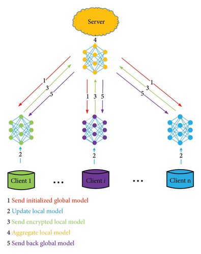
We adopted the necessary privacy protection mechanisms in HFL to transfer local/global models, thus ensuring the security of the entire training process.

3.2. ISV

The ISV is an improved concept based on the classical SV [36] and is primarily used to manage data with uncertainty or interval values. In the classical SV, the contributions of participants are determined by calculating their marginal contributions in different collaborative situations. Within the ISV framework, the contribution of each participant is extended into an interval [a_i, b_i], where a_i and b_i are the minimum and maximum contributions of the participants in different scenarios, respectively. For example, consider three participants, A, B, and C, cooperating to complete a task. The resulting benefit is v(s), where S represents a subset of the participants. In the classical SV, we calculate the marginal contribution of each participant and their average. Meanwhile, in ISV, we calculate the marginal contribution interval of each participant in different contexts and provide an interval for the participant’s contribution. The ISV introduces intervals to address uncertainty, thus rendering it more flexible and adaptable to complex situations in practical applications. It is particularly suitable for problems involving uncertain data or risk assessments and provides more information and robustness to the calculations contributed by participants as compared with the classical SV.

3.3. Matrix Semitensor Product

Matrix semitensor products are the main research tools for state-space methods in logical systems and have been widely applied for solving nonlinear problems. Next, we briefly introduce the definitions, properties, and other aspects of a matrix semitensor product.

Definition 1 (Matrix semitensor product) [46]. If matrix and matrix are provided, then the semitensor product of matrices and is defined as follows:

()

where ⊗ represents the tensor product of matrices and t is the least common multiple of n and p, i.e., t = lcm(n, p).

The matrix semitensor product is an extension of matrix multiplication that extends ordinary matrix multiplication to the multiplication of any two matrices. When n = p, the matrix semitensor product is a regular matrix multiplication. Unless otherwise specified, matrix multiplication mentioned herein refers to a semitensor product, and ⋉ is omitted.

Definition 2 (Permutation matrix). If permutation matrix , then the following is satisfied:

()

Because is a sparse matrix, it is typically expressed in concise form, W_{[m, n]} = δ_mn[1 1 + m ⋯ 1 + (n − 1)m ⋯ mm + m ⋯ m + (n − 1)m]. The semitensor product of the matrices satisfies pseudocommutativity [47]. According to Definition 2, vector multiplication can be exchanged with the semitensor product, i.e., .

In the study of finite-interval games, the utility functions of participants can be regarded as pseudo-Boolean (logic) functions. The following proposition provides an algebraic expression for the pseudological function.

Proposition 1 [48]. Let be a pseudological function, and if a unique 1 × 2ⁿ-matrix exists that satisfies , then is known as the unique structural matrix of the pseudological function f.

Based on Proposition 1, Lemma 1 can be obtained:

Lemma 1. Let be a pseudological interval function. If a unique interval matrix exists that satisfies , then is known as the unique structural matrix of the pseudological interval function f.

4. Methodology

To address the challenges posed by the differences and uncertainties in the contribution levels of participants from different data sources for mechanism design, we propose the IntFedSV contribution evaluation mechanism for the first time in HFL scenarios. The IntFedSV is a variant of the ISV for FL scenarios. Unlike previous methods [19, 20], the core idea of the IntFedSV is to extend the classical single-point SV to a finite interval using the different utility values of the subfederation in different iteration rounds and introducing the discount factor to adjust the final allocation effect of the IntFedSV. This method is advantageous as it fully utilizes the fault tolerance of the ISV to offset the adverse problems caused by the differences and uncertainties of the participants. Ultimately, the participants’ contribution levels are within a more stable range. Additionally, to improve the computational efficiency, we utilized a matrix semitensor product-based method to compute the IntFedSV.

4.1. System Workflow

As shown in Figure 2, the workflow of the proposed IntFedSV system comprises primarily the following five steps:

Step 1: FL. In each iteration round t ∈ {0, 1, ⋯, T − 1}, all n participants i ∈ N = {1, 2, ⋯, n} perform the FL task based on the steps outlined in Section 3.1 to obtain a local model .
Step 2: The subfederation model is approximately reconstructed [19]. The server utilizes the gradient information obtained from the FL task to approximately reconstruct the model for subfederation S. Here, .
Step 3: Evaluate the utility of the submodel. The server maps the subfederation model based on a preset utility function to obtain the utility value of the submodels. The utility function maps the data of each participant to the performance metrics (accuracy [20] or loss [49]) of the model trained on the data.
Step 4: Determine the upper and lower limits of the utility interval. The server traverses the utility value of all subfederated models in each iteration round t and identifies the utility interval , where S ∈ 2^N.
Step 5: Calculate the IntFedSV (which will be defined later.). The server uses the matrix semitensor product method to calculate the IntFedSV Φ(v) of the participants.

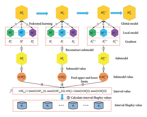
4.2. Definition of IntFedSV

Without loss of generality, we used a binary structure (N, v) to denote interval federated cooperative games, where the set of finite elements N = {1, 2, ⋯, n} denotes the set of participants for FL, and the feature function satisfies v(∅) = [0, 0], where represents the real number. All subsets of N are denoted as 2^N = {S|S⊆N}. For ∀S ∈ 2^N, v(M_S) is the utility function of the subfederated model M_S, and the function value is an interval denoted as , where S ∈ 2^N, t ∈ {0, 1, ⋯, T − 1}. When , the interval federated cooperative game degenerates into the classical federated cooperative game.

Based on [38], the SV of interval federated cooperative games is expressed as

()

where

denotes the utility function of the subfederated model, v(M_S∪i) − v(M_S) denotes the marginal contribution for participant i, and

However, in many FL scenarios, the total utility is typically affected by various uncertain factors beyond the performance of the federated model. To measure the contribution level of the participants more fairly, we formally define the IntFedSV based on the ISV with a discount factor by Fei, Li, and Ye [39].

Definition 3 (IntFedSV). Let (N, v) denote the interval federated cooperative game, N = {1, 2, ⋯, n} denote the set of participants for FL, and denote the interval value of the utility for subfederated model M_S. Therefore, the IntFedSV for participant i can be expressed as

()

where λ ∈ [0, 1] denotes the discount factor. When λ = 1, the discounted SV of (7) degenerates into (6). Meanwhile, λ = 0 indicates that the participants have evenly distributed the total utility, i.e., Φ_i(v) = v(N)/n. Interval cooperative games is an extension of the classical cooperative game; therefore, the IntFedSV satisfies the efficiency, symmetry, and additivity [39].

4.3. IntFedSV Calculation Method Based on Matrix Semitensor Product

If we calculate the IntFedSV directly using (7) in Definition 3, then the time complexity of the calculation is , where n is the number of participants and T is the maximum iteration round. This method is time-consuming.

To reduce the time required for calculating the IntFedSV, we introduce the matrix semitensor product theory. We first present the calculation method and then provide the relevant proof. Theorem 1 provides a convenient method for calculating the IntFedSV. Please refer to Appendix A for the detailed proof.

Theorem 1. For an interval federated cooperative game (N, v), where N = {1, 2, ⋯, n} is the set of participants and is the structural matrix of the interval utility function v(M_S), the SV of the interval federated cooperative games can be calculated as follows:

()

where K and F are the Shapley matrices. K = [K₁, K₂, ⋯K_N], F = [F₁, F₂, ⋯F_N], and

, where S ∈ 2^N, t ∈ {0, 1, ⋯, T − 1}.

According to Theorem 1, the time complexity of calculating the IntFedSV based on the matrix semitensor in (8) is reduced to . Additionally, we introduce truncation techniques to accelerate the computational efficiency of the IntFedSV (which will be discussed later).

4.4. IntFedSV Algorithm

Algorithm 1 presents the pseudocode of the proposed method. In general, the algorithm comprises two components: the server and client. In the first line, the server randomly initializes the global model and submodels. For each iteration round t, in Lines 4–9, the server aggregates the global model. In Lines 11–15, the server uses the participant’s gradient values during FL training to reconstruct the subfederation model, which effectively avoids the resource waste caused by retraining the subfederation. Additionally, we set a round-truncated threshold τ > 0 during the training process to improve the speed of evaluating the utility of the submodels. In Lines 18–23, the server first uses the evaluation function to obtain the utility interval of the subfederated model and then uses the IntFedSV formula (Definition 3) to calculate the contribution values of each participant. In Lines 24–30, the client uses the classic minibatch stochastic gradient descent algorithm to train the local model on a local dataset [19].

Algorithm 1: IntFedSV.

Input: Participants set N, local data D_i, training rounds T, local minibatch size B, local epochs E, learning rate η, evaluation function v, round-truncated threshold τ, discount factor λ, and Shapley matrices K and F.
Output: IntFedSV Φ(v).
Server executes:
1. Initialize global model M⁰ and submodel
2. for each round t = 0, 1, …, T − 1do
3. # Aggregate global model
4. Send global model M^t to all participants
5. for each participant i in parallel do
6.
7.
8. end for
9.
10. # Approximate reconstruction submodel
11. if|v(M^t+1) − v(M^t)| > τthen
12. for each subset S⊆Ndo
13. +
14. end for
15. end if
16. end for
17. # Calculate interval federated Shapley Value (IntFedSV)
18. Initialize the structural matrix
19. for each S⊆Ndo
20.
21. end for
22.
23. returnM^T and Φ(v)
ClientUpdate(i, M^t):
24. Initialize local model to global model M^t
25. for each local epoch e = 0, 1, …, E − 1do
26. for batch B ∈ D_ido
27.
28. end for
29. end for
30. return

4.5. Time Complexity Analysis

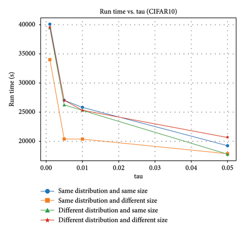
As presented in Section 4.2, the time complexity of calculating the IntFedSV Φ(v) based on the matrix semitensor product is . After introducing the truncated threshold τ (in Section 4.4), the time complexity of calculating the IntFedSV is between and . Specifically, a smaller truncated threshold τ implies fewer truncated rounds and a time complexity closer to . In the opposite case, the time complexity is closer to . However, the actual time complexity is closely related to the distribution and size of the datasets.

5. Experiments

To verify the performance of the proposed IntFedSV contribution evaluation method in practical engineering applications, we conducted FL simulation experiments using an open-source distributed learning simulator [20] on the MNIST [50], CIFAR10 [49], AG_NEWS [51], and IMDB [52] datasets. The MNIST dataset comprises 70,000 black and white images containing 0–9 handwritten digits, each measuring 28 × 28 pixels. We used 60,000 and 10,000 images for training and testing, respectively. The CIFAR10 dataset contains 60,000 color images measuring 32 × 32 pixels from 10 categories, where 50,000 and 10,000 images were specified for training and testing, respectively. The MNIST and CIFAR10 datasets are public datasets commonly used for image classification. The AG-NEWS dataset contains 120,000 training samples and 7600 testing samples from four major categories. Each category features 30,000 and 1900 samples in the training and testing sets, respectively. The IMDB dataset contains 50,000 movie reviews, of which 25,000 were used for training and 25,000 for testing. Both the training and testing sets contained 50% positive and 50% negative comments. AG-NEWS and IMDB are public datasets commonly used for text classification in NLP. The experiment was conducted on a Linux system equipped with 32G main memory and a 12G RTX 4070Ti graphics card. The source code and partial results are available at https://github.com/yunshuichanxin520/distributed_learning_simulator. We assumed that six participants participated in the FL model training.

5.1. Dataset Settings

For the four datasets mentioned above, we considered four iid and non-iid scenarios each for the distribution and size of the datasets.

1.
Same distribution and same size (iid): For each dataset, we randomly apportioned the dataset (training and testing sets) into six segments of the same size to ensure that each participant obtained the same data distribution.
2.
Same distribution and different sizes (iid): For each dataset, we randomly sampled from the entire training set based on a preset ratio while ensuring that each participant had the same amount of data for each class label. That is, the ratios of Participants 1 and 2 were 10%, those of Participants 3 and 4 were 50%, and those of Participants 5 and 6 were 90%.
3.
Different distributions and same size (non-iid): Each dataset was randomly apportioned into six segments of the same size. Subsequently, the labels were “flipped” based on the preset ratio to add noise. That is, the ratios of Participants 1 and 2 were 1%, those of Participants 3 and 4 were 10%, and those of Participants 5 and 6 were 20%. Here, “flip” refers to randomly shuffling the labels of each sample (image/comment) into incorrect values.
4.
Different distributions and different sizes (non-iid): We used the common Dirichlet distribution to apportion each dataset. The setting and range of concentration parameter α > 0 are crucial for controlling the data size and distribution. The larger the value of α, the more concentrated the generated distribution is. The smaller the value of α, the more dispersed the generated distribution is [53]. To generate datasets of different sizes and distributions, we set α to 0.5.

5.2. Comparison Algorithms

We compared the proposed IntFedSV contribution evaluation mechanism with three advanced baseline methods. Unless otherwise specified, the relevant parameters of the comparative algorithm uses the optimal parameter settings presented in the original paper.

1.
TMR-Shapley [29]. This method is an extension of the MR method presented in [19]. It controls the weight of each participant’s SV by adding a decay factor and introduces a truncated threshold to reduce unnecessary submodel reconstruction.
2.
GTG-Shapley [20]. In this method, two truncated techniques guided by Monte Carlo sampling between and within rounds are proposed to further improve the computational efficiency of SV-based contribution indices.
3.
ComFedSV [47]. This method is an improvement of the FedSV [14]. To reduce computational costs, a certain number of participants are selected for model training in each round, which results in an incomplete utility matrix. Hence, the low-rank matrix is solved to complete the utility matrix and then the SV is calculated.

5.3. Tasks and Parameter Settings

In our setup, the contribution evaluation mechanism is independent of FL model training. Therefore, to ensure the optimal training effect of the FL model, we referred to the method presented in [20, 54] to set the optimal hyperparameters related to the training of the FL model (as listed in Table 1), during which the client selected the best result for uploading based on the validation set in five epochs. We used the test accuracy of the model as the value of the utility function. For text classification tasks, word embeddings were initialized using glove word embeddings [55]. For the ComFedSV, we set the rate of participants to 0.5, which implies that three clients participate in the FL model training and contribution evaluation in each round. We will conduct ablation experiments on the hyperparameters (round-truncated threshold τ and discount factor λ) related to the performance of the contribution evaluation mechanism in the future. In the comparative experiment section, for each dataset, we set τ to 0.005; additionally, we set λ to 1 (From Definition 3, one can infer that when λ = 1, the discounted SV degenerates into a classical SV. Since other baseline methods used for comparison are classical SVs, we set λ = 1).

Table 1. Hyperparameter settings for different tasks.

Dataset	Participants	Model	Optimizer	Batch size	Learning rate	Rounds	Epochs	Parameters
MNIST	6	LeNet5	SGD	64	0.01	20	5	60,000
CIFAR10		densenet40			0.1	100		0.17 million
AG_NEWS		Classification model with two transformer encoder layers			0.01			17 million
IMDB		Classification model with two transformer encoder layers			0.01			17 million

5.4. Evaluation Metric

To verify the superiority of the proposed mechanism, we used the standard deviation of the SV from different participants in the same set of experiments to measure the performance of different evaluation mechanisms. The smaller the standard deviation, the smaller the difference in the SV for the participants is, and the higher the stability of the contribution evaluation mechanism is. For the IntFedSV, we calculated the standard deviation of the interval median,

()

where φ_i represents the SV of participant i and

represents the mean SV of n participants.

5.5. Analysis of Experimental Results

Figures 3, 4, 5, and 6 show the variation in the SV for each participant under different settings for the four datasets. As shown in the figures, the proposed IntFedSV contribution evaluation mechanism extends the classical single-point SV to a finite interval. However, the other baseline methods calculated a single-point SV. To facilitate comparison, we selected the median value of the IntFedSV interval as an example (dashed blue line). Intuitively, the SV calculated by the TMR-Shapley and GTG-Shapley mechanisms fluctuated significantly, whereas the IntFedSV and ComFedSV were relatively stable, particularly on the MNIST, AG-NEWS, and IMDB datasets.

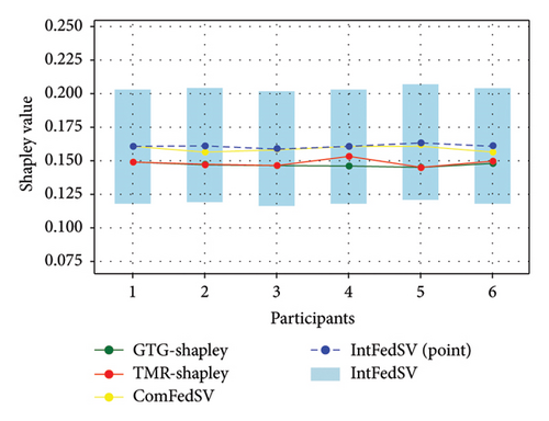
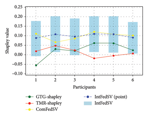
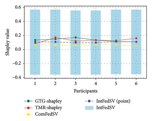
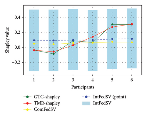
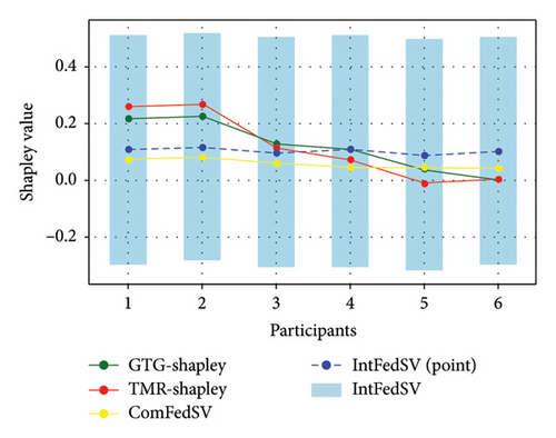
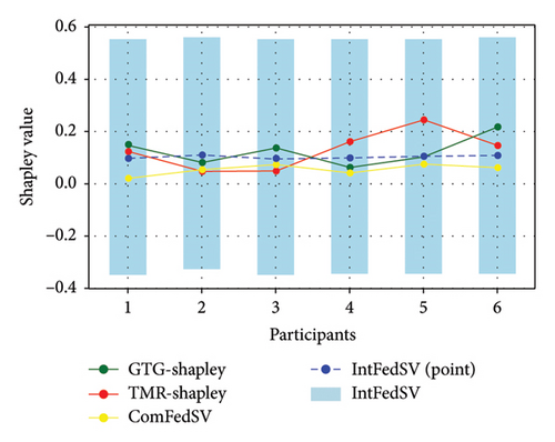
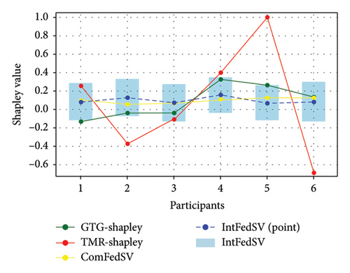
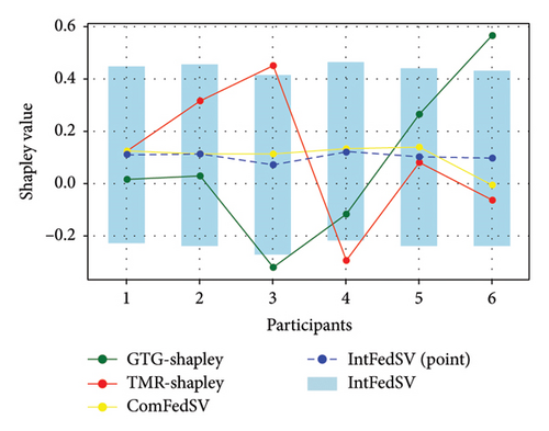
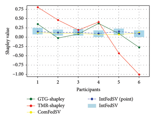
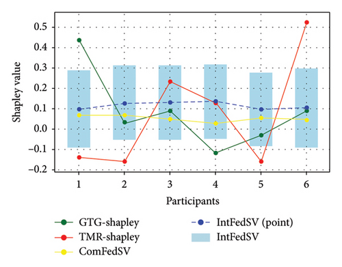
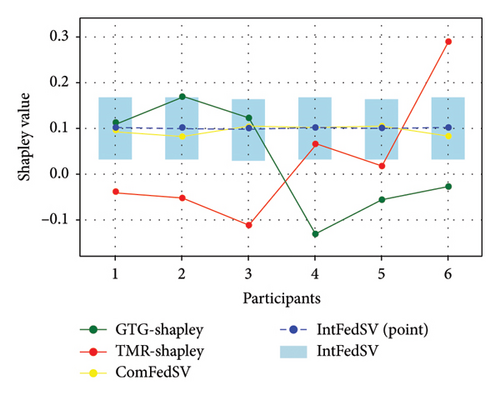
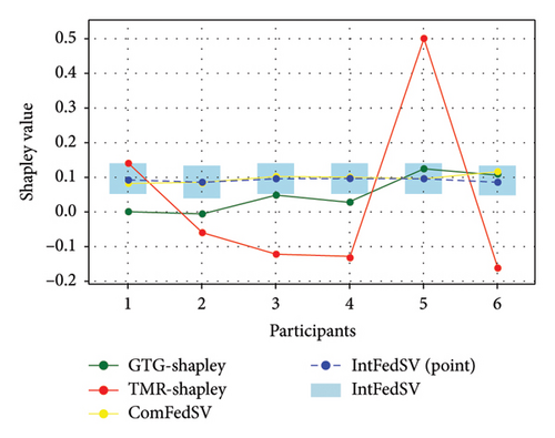
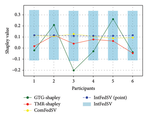
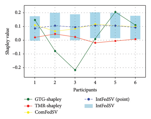
To further quantify the performances of the different evaluation mechanisms, we calculated the standard deviation/improvement rate of the participants’ SVs for each mechanism under different settings in the datasets. As shown in Tables 2, 3, 4, and 5, the standard deviation of the proposed IntFedSV evaluation mechanism was the minimum under the different settings of the four datasets. Additionally, its minimum and maximum improvement rates were 11.83% and 99.00%, respectively. This demonstrates the superiority of the proposed mechanism in terms of stability.

Table 2. Standard deviation/improvement rate of SV for each mechanism on MNIST.

CIFAR10 settings	IntFedSV	GTG-Shapley	TMR-Shapley	ComFedSV
Same distribution and same size	0.0011	0.0014/21.43%	0.0027/59.26%	0.0020/45.00%
Same distribution and different size	0.0417	0.1147/63.64%	0.1981/78.95%	0.1334/68.74%
Different distribution and same size	0.0024	0.1593/98.49%	0.0519/95.38%	0.0117/79.49%
Different distribution and different size	0.0087	0.0393/77.86%	0.0205/57.56%	0.0179/51.40%

Table 3. SV standard deviation/improvement rate for each mechanism on CIFAR10.

CIFAR10 settings	IntFedSV	GTG-Shapley	TMR-Shapley	ComFedSV
Same distribution and same size	0.0059	0.0218/72.94%	0.0272/78.31%	0.0069/14.49%
Same distribution and different size	0.0100	0.1538/93.50%	0.1441/93.06%	0.0150/33.33%
Different distribution and same size	0.0085	0.0833/89.80%	0.1107/92.32%	0.0160/46.88%
Different distribution and different size	0.0058	0.0516/88.76%	0.0681/91.48%	0.0169/65.68%

Table 4. SV standard deviation/improvement rate for each mechanism on AG_NEWS.

AG_NEWS settings	IntFedSV	GTG-Shapley	TMR-Shapley	ComFedSV
Same distribution and same size	0.0221	0.1682/86.86%	0.5445/95.94%	0.0336/34.23%
Same distribution and different size	0.0168	0.2800/94.00%	0.2414/93.04%	0.0485/65.36%
Different distribution and same size	0.0231	0.2245/89.71%	0.6141/96.24%	0.0262/11.83%
Different distribution and different size	0.0153	0.1732/91.17%	0.2536/93.97%	0.0173/12.27%

Table 5. Standard deviation/improvement rate of SV for each mechanism on IMDB.

IMDB settings	IntFedSV	GTG-Shapley	TMR-Shapley	ComFedSV
Same distribution and same size	0.0013	0.1090/98.81%	0.1294/99.00%	0.0092/85.87%
Same distribution and different size	0.0037	0.0485/92.37%	0.2318/98.40%	0.0124/70.16%
Different distribution and same size	0.0024	0.1593/98.49%	0.0519/95.38%	0.0117/79.49%
Different distribution and different size	0.0088	0.1462/93.98%	0.0206/57.28%	0.0180/51.11%

In general, the IntFedSV ensured that the contribution levels of the participants remained stable. Compared with the unique allocation of a single-point SV, the utility interval demonstrated greater fault tolerance and incentive, which encouraged participants to join the FL alliance more effectively. In particular, under uncertain environments, the advantage of the IntFedSV was more significant.

5.6. Ablation Experiments

5.6.1. Ablation Experiment of Discount Factor

To further investigate the effect of the discount factor on the contribution level of the participants, we used the CIFAR10 and IMDB datasets to examine the IntFedSV corresponding to different discount factors. Specifically, we set the values of λ to 0, 0.2, 0.4, 0.6, 0.8, and 1. Similarly, we considered four scenarios for the datasets. The experimental results are shown in Figures 7 and 8.

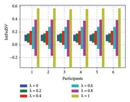
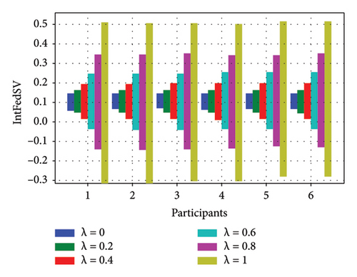
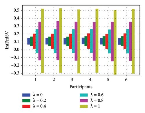
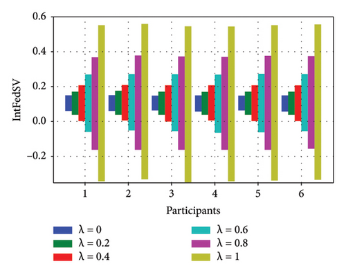
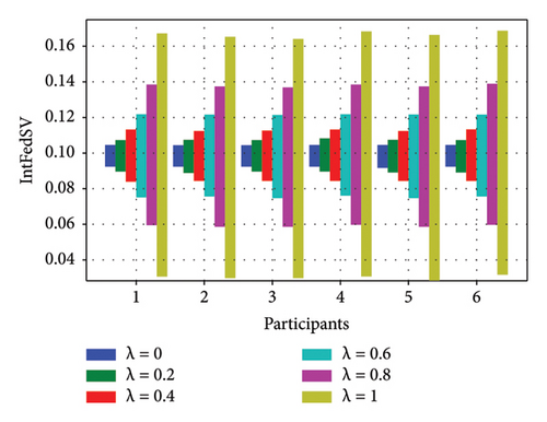
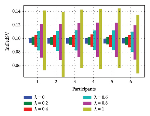
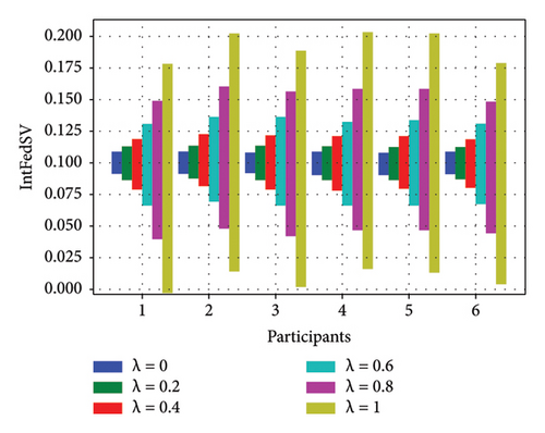
Based on Figures 7 and 8, under the four settings of the four datasets, the IntFedSV interval length of the participants increased significantly with the discount factor, although the increase in magnitude varied. When λ = 0, the same IntFedSV results were obtained for each participant, which is consistent with the findings presented in the theoretical section. Therefore, we can control the utility interval and fault tolerance of the participants by setting the appropriate discount factors.

5.6.2. Ablation Experiment of Round-Truncated Threshold

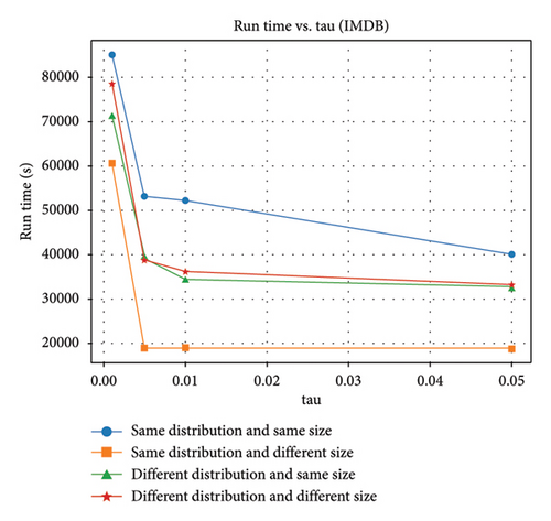
To further investigate the effect of the round-truncated threshold on the contribution evaluation mechanisms, we used the CIFAR10 and IMDB datasets to examine the IntFedSV corresponding to different round-truncated thresholds. Specifically, we set the values of τ to 0.001, 0.005, 0.01, and 0.05. Similarly, we considered four scenarios for the datasets. The experimental results are shown in Figures 9 and 10.

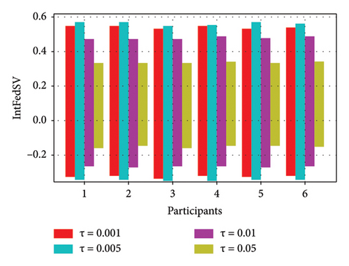
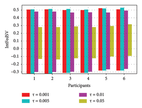
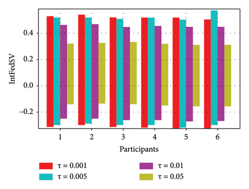
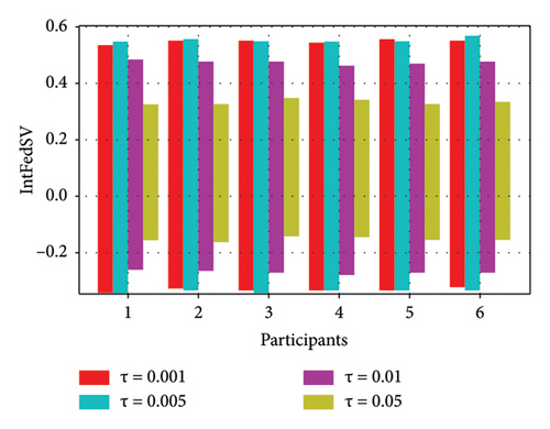
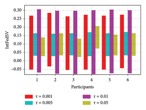
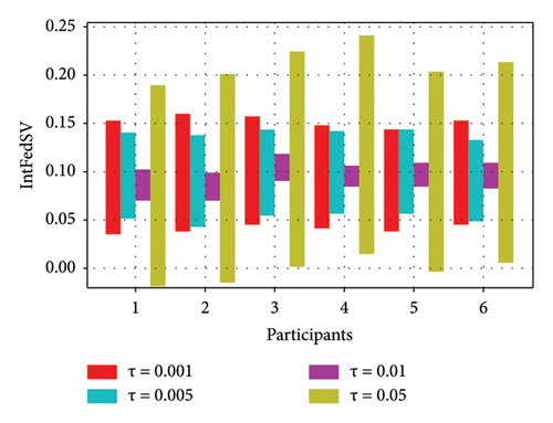
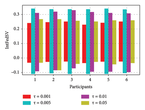
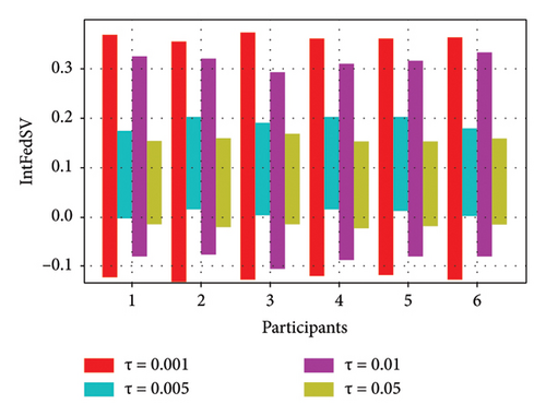
As shown in Figures 9 and 10, the round-truncated threshold significantly affected the IntFedSV of the participants in all four scenarios. However, the effect varied depending on the dataset settings. As presented in Section 4.5, the larger the round-truncated threshold, the shorter the algorithm runtime is. To further investigate the effect of the round-truncated threshold on the algorithm runtime, we analyzed the variation of Algorithm 1’s runtime with a round-truncated threshold under different settings of the dataset. As shown in Figures 11 and 12, the larger the round-truncated threshold, the shorter the algorithm runtime is. Therefore, in actual FL experimental scenarios, we should comprehensively consider the IntFedSV and runtime to select an appropriate round-truncated threshold.

In summary, the superiority of the proposed IntFedSV contribution evaluation mechanism was demonstrated through comparative experimental results with the result of baseline methods on public datasets. In uncertain environments, the advantage of the IntFedSV was more significant. In further ablation experiments, we investigated the effects of the discount factor and round-truncated threshold on the experimental results. The results showed that the IntFedSV interval length of the participants increased significantly with the discount factor, although the increase in magnitude varied. Therefore, we can control the utility interval and fault tolerance of the participants by setting the appropriate discount factors. The larger the round truncation threshold, the shorter the algorithm runtime is. Therefore, in practical FL applications, we should comprehensively consider the IntFedSV and runtime to select the appropriate round truncation threshold. This study fills the research gap pertaining to the application of interval SVs in the design of FL contribution evaluation mechanisms and contributes positively to the promotion of FL engineering applications.

6. Conclusion

To address the challenges posed by the differences and uncertainties in the contribution levels of participants from different data sources, we proposed an IntFedSV mechanism for HFL. This mechanism is advantageous as it fully utilizes the fault tolerance of the ISV to offset the adverse problems caused by the differences and uncertainties of the participants. Ultimately, the participants’ contribution levels were within a more stable range. Second, to further accelerate computational efficiency, we introduced a matrix semitensor product method to calculate the IntFedSV. Finally, extensive experiments on public datasets demonstrated that the proposed mechanism can effectively evaluate the contribution level of the participants. Compared with the classic single-point SV, the IntFedSV offers greater fault tolerance and incentive, which allows it to promote FL engineering applications more effectively. Under uncertain environments, the advantage of the IntFedSV is more significant.

However, our study presents some limitations. First, the IntFedSV must traverse all 2ⁿ subsets in each round of utility evaluation, and the computational complexity of the algorithm is relatively high. Although we adopted the round-truncated technique and the matrix semitensor method to improve the computational efficiency of the IntFedSV, the risk of an exponential explosion remains. Second, the real-time requirements of FL systems are gradually increasing. However, we did not combine the IntFedSV allocation results with a new round of resource allocation to form a dynamic feedback mechanism. In the future, we will address the issues of utilizing IntFedSV to allocate a new round of data, computing power, and communication resources, as well as develop a real-time online IntFedSV contribution evaluation and resource allocation system.

Conflicts of Interest

The authors declare no conflicts of interest.

Author Contributions

Tianxu Cui: investigation, conceptualization, methodology, data curation, formal analysis, writing – original draft, and writing – review and editing. Ying Shi: conceptualization, methodology, supervision, and writing – review and editing. Wenge Li: methodology, formal analysis, writing – original draft, and visualization. Rijia Ding: methodology, writing – review and editing, funding acquisition, and supervision. Qing Wang: data curation, formal analysis, writing – original draft, and visualization.

Funding

This work was supported by the National Key R&D Program (No. 2022YFF0607404) and the Fundamental Research Funds for the Central Universities (Ph.D. Top Innovative Talents Fund of CUMTB) (No. BBJ2024077).

Acknowledgments

Appendix A: Proof of Theorem 1

Proof 1. Considering interval federated cooperative games (N, v), for ∀ S ∈ 2^N, v(M_S) is the utility function of the subfederated model M_S. Therefore, we construct , where

()

According to Lemma 1, the utility function can be expressed as

()

where the structural matrix

. Next, we apply matrix semitensor product theory to transform the utility function of interval federated cooperative games into a matrix form.

First, we consider the marginal contribution v(M_S∪i) − λv(M_S) in Equation (7). If , then from the permutation matrix (Definition 2), we can obtain

()

Second, using the method of Cheng et al. [46], we construct a vector sequence , i.e.,

()

where

Lemma 2 [46]. Let S ⊂ N = {x₁, x₂, ⋯, x_n}, if , then (A.7)

Where denotes the jth component of a_n.

According to Lemma 2, let ; subsequently, we construct a vector sequence , where

()

For convenience, we segment vector γ into k-block vectors sequentially, with j = 1, 2, 2², ⋯, 2ⁿ⁻¹, as follows:

()

where

Therefore, based on Equations (A.5) and (A.7), one can infer from Equation (7) that

()

Notably,

()

Therefore, for ∀i = 1, 2, ⋯, n, we construct matrix Λ_i as follows:

()

Based on the pseudocommutative property of the matrix semitensor product, the following can be obtained:

()

Then,

()

where E_i is a 2ⁿ-dimensional column vector.

Similarly,

()

Then, for ∀i = 1, 2, ⋯, n, we construct matrix Γ_i as follows:

()

Thus, we can obtain

()

where F_i is a 2ⁿ-dimensional column vector. Combining Equations (A.13) and (A.15), one can write Equation (A.9) as follows:

()

Thus, Theorem 1 is proven.

Nomenclature.

To facilitate understanding, we have summarized the main abbreviations and mathematical symbols used in this section in Table A1.

Table A1. Abbreviations and mathematical symbols.

Abbreviations/symbols	Meaning
FL	Federated learning
HFL	Horizontal federated learning
SV	Shapley value
ISV	Interval Shapley value
IntFedSV	Interval federated Shapley value
i ∈ N = {1, 2, ⋯, n}	Participants (clients)
t ∈ {0, 1, ⋯, T − 1}	Global iteration rounds
D_i	Dataset owned by each participant
	Local model
M^t	Global model of all participant set N in the tth round
	Gradient of local model
∆^t	Gradient of global model
	Global model of subfederation S in the tth round
	Utility value of subfederation S in the tth round
M_S	Subfederated model
	Interval utility function of subfederated model M_S
(N, v)	Interval federated cooperative games
N = {1, 2, ⋯, n}	Set of participants for FL
	Feature function
Φ_i(v)	IntFedSV for participant i
λ ∈ [0, 1]	Discount factor
τ > 0	Round-truncated threshold
	Structural matrix of interval utility function v(M_S)
K and F	Shapley matrix

Open Research

Data Availability Statement

The four datasets used in this paper are public datasets and are only used for scientific research.

References

1 Saggi M. K. and Jain S., A Survey Towards an Integration of Big Data Analytics to Big Insights for Value-Creation, Information Processing & Management. (2018) 54, no. 5, 758–790, https://doi.org/10.1016/j.ipm.2018.01.010, 2-s2.0-85041554154.
10.1016/j.ipm.2018.01.010
Web of Science® Google Scholar
2 Hoofnagle C. J., Van Der Sloot B., and Borgesius F. Z., The European Union General Data Protection Regulation: What it is and What it Means, Information and Communications Technology Law. (2019) 28, no. 1, 65–98, https://doi.org/10.1080/13600834.2019.1573501, 2-s2.0-85061524633.
10.1080/13600834.2019.1573501
Web of Science® Google Scholar
3 Ke T. T. and Sudhir K., Privacy Rights and Data Security: GDPR and Personal Data Markets, Management Science. (2023) 69, no. 8, 4389–4412, https://doi.org/10.1287/mnsc.2022.4614.
10.1287/mnsc.2022.4614
Web of Science® Google Scholar
4 Xu J., Hong N., Xu Z. et al., Data-Driven Learning for Data Rights, Data Pricing, and Privacy Computing, Engineering. (2023) 25, 66–76, https://doi.org/10.1016/j.eng.2022.12.008.
10.1016/j.eng.2022.12.008
Google Scholar
5 McMahan B., Moore E., Ramage D., Hampson S., and Arcas B. A., Communication-Efficient Learning of Deep Networks From Decentralized Data, Artificial Intelligence and Statistics. (2017) PMLR, New York, NY, 1273–1282.
Google Scholar
6 Li P., Li J., Huang Z. et al., Multi-Key Privacy-Preserving Deep Learning in Cloud Computing, Future Generation Computer Systems. (2017) 74, 76–85, https://doi.org/10.1016/j.future.2017.02.006, 2-s2.0-85018906248.
10.1016/j.future.2017.02.006
Web of Science® Google Scholar
7 Liu W., Zhang Y., Han G., Cao J., Cui H., and Zheng D., Secure and Efficient Smart Healthcare System Based on Federated Learning, International Journal of Intelligent Systems. (2023) 2023, no. 1, https://doi.org/10.1155/2023/8017489.
10.1155/2023/8017489
Google Scholar
8 Xing F., Financial Risk Tolerance Profiling from Text, Information Processing & Management. (2024) 61, no. 4, https://doi.org/10.1016/j.ipm.2024.103704.
10.1016/j.ipm.2024.103704
Google Scholar
9 Zhang J., Ning Z., and Xue F., A Two-Stage Federated Optimization Algorithm for Privacy Computing in Internet of Things, Future Generation Computer Systems. (2023) 145, 354–366, https://doi.org/10.1016/j.future.2023.03.042.
10.1016/j.future.2023.03.042
Google Scholar
10 Shi Y., Yu H., and Leung C., Towards Fairness-Aware Federated Learning, IEEE Transactions on Neural Networks and Learning Systems. (2024) 35, no. 9, 11922–11938, https://doi.org/10.1109/TNNLS.2023.3263594.
10.1109/TNNLS.2023.3263594
PubMed Google Scholar
11 Wang G., Dang C. X., and Zhou Z., Measure Contribution of Participants in Federated Learning, 2019 IEEE International Conference on Big Data (Big Data), December 2019, Los Angeles, CA, IEEE, 2597–2604, https://doi.org/10.1109/BigData47090.2019.9006179.
10.1109/BigData47090.2019.9006179
Google Scholar
12 Arafeh M., Ould-Slimane H., Otrok H., Mourad A., Talhi C., and Damiani E., Data Independent Warmup Scheme for Non-IID Federated Learning, Information Sciences. (2023) 623, 342–360, https://doi.org/10.1016/j.ins.2022.12.045.
10.1016/j.ins.2022.12.045
Google Scholar
13 Ye M., Fang X., Du B., Yuen P. C., and Tao D., Heterogeneous Federated Learning: State-of-the-Art and Research Challenges, ACM Computing Surveys. (2023) 56, no. 3, 1–44, https://doi.org/10.1145/3625558.
10.1145/3625558
Google Scholar
14 Wang T., Rausch J., Zhang C., Jia R., and Song D., A Principled Approach to Data Valuation for Federated Learning, Lecture Notes in Computer Science. (2020) 153–167, https://doi.org/10.1007/978-3-030-63076-8_11.
10.1007/978-3-030-63076-8_11
Google Scholar
15 Lin W., Xu Y., Liu B., Li D., Huang T., and Shi F., Contribution-Based Federated Learning Client Selection, International Journal of Intelligent Systems. (2022) 37, no. 10, 7235–7260, https://doi.org/10.1002/int.22879.
10.1002/int.22879
Google Scholar
16 Liu P., Xu X., and Wang W., Threats, Attacks and Defenses to Federated Learning: Issues, Taxonomy and Perspectives, Cybersecurity. (2022) 5, no. 1, https://doi.org/10.1186/s42400-021-00105-6.
10.1186/s42400-021-00105-6
Google Scholar
17 Yu H., Liu Z., Liu Y. et al., A Sustainable Incentive Scheme for Federated Learning, IEEE Intelligent Systems. (2020) 35, no. 4, 58–69, https://doi.org/10.1109/MIS.2020.2987774.
10.1109/MIS.2020.2987774
Web of Science® Google Scholar
18 Donahue K. and Kleinberg J., Model-sharing Games: Analyzing Federated Learning Under Voluntary Participation, Proceedings of the AAAI Conference on Artificial Intelligence. (2021) 35, no. 6, 5303–5311, https://doi.org/10.1609/aaai.v35i6.16669.
10.1609/aaai.v35i6.16669
Google Scholar
19 Song T., Tong Y., and Wei S., Profit Allocation for Federated Learning, 2019 IEEE International Conference on Big Data (Big Data), December 2019, Los Angeles, CA, IEEE, 2577–2586, https://doi.org/10.1109/BigData47090.2019.9006327.
10.1109/BigData47090.2019.9006327
Google Scholar
20 Liu Z., Chen Y., Yu H., Liu Y., and Cui L., Gtg-Shapley: Efficient and Accurate Participant Contribution Evaluation in Federated Learning, ACM Transactions on intelligent Systems and Technology (TIST). (2022) 13, no. 4, 1–21, https://doi.org/10.1145/3501811.
10.1145/3501811
Web of Science® Google Scholar
21 Zhang J., Li C., Robles-Kelly A., and Kankanhalli M., Hierarchically Fair Federated Learning, 2020, https://arxiv.org/abs/2004.10386.
Google Scholar
22 Pandey S. R., Tran N. H., Bennis M., Tun Y. K., Manzoor A., and Hong C. S., A Crowdsourcing Framework for on-Device Federated Learning, IEEE Transactions on Wireless Communications. (2020) 19, no. 5, 3241–3256, https://doi.org/10.1109/TWC.2020.2971981.
10.1109/TWC.2020.2971981
Web of Science® Google Scholar
23 Ghosh B., Basu D., Huazhu F. et al., Don′t Forget What I Did?: Assessing Client Contributions in Federated Learning, 2024, https://arxiv.org/abs/2403.07151.
Google Scholar
24 Lyu L., Yu J., Nandakumar K. et al., Towards Fair and Privacy-Preserving Federated Deep Models, IEEE Transactions on Parallel and Distributed Systems. (2020) 31, no. 11, 2524–2541, https://doi.org/10.1109/TPDS.2020.2996273.
10.1109/TPDS.2020.2996273
Web of Science® Google Scholar
25 Chen Y. C., Chen H. W., Wang S. G., and Chen M. S., SPACE: Single-Round Participant Amalgamation for Contribution Evaluation in Federated Learning, Advances in Neural Information Processing Systems. (2024) 36.
PubMed Google Scholar
26 Yang X., Xiang S., Peng C. et al., Federated Learning Incentive Mechanism Design Via Shapley Value and Pareto Optimality, Axioms. (2023) 12, no. 7, https://doi.org/10.3390/axioms12070636.
10.3390/axioms12070636
PubMed Google Scholar
27 Tajabadi M. and Heider D., Fair Swarm Learning: Improving Incentives for Collaboration by a Fair Reward Mechanism, Knowledge-Based Systems. (2024) 304, https://doi.org/10.1016/j.knosys.2024.112451.
10.1016/j.knosys.2024.112451
Google Scholar
28 Shapley L. S., A Value for N-Person Games, Contributions to the Theory of Games. (1953) 2, no. 28, 307–317, https://doi.org/10.1515/9781400829156-012.
10.1515/9781400829156-012
Google Scholar
29 Wei S., Tong Y., Zhou Z., and Song T., Efficient and Fair Data Valuation for Horizontal Federated Learning, Lecture Notes in Computer Science. (2020) 139–152, https://doi.org/10.1007/978-3-030-63076-8_10.
10.1007/978-3-030-63076-8_10
Google Scholar
30 Jia R., Dao D., Wang B. et al., Towards Efficient Data Valuation Based on the Shapley Value, The 22nd International Conference on Artificial Intelligence and Statistics. (2019) 89, 1167–1176.
Google Scholar
31 Zhao J., Zhu X., Wang J., and Xiao J., Efficient Client Contribution Evaluation for Horizontal Federated Learning, ICASSP 2021-2021 IEEE International Conference on Acoustics, Speech and Signal Processing (ICASSP), June 2021, Toronto, ON, Canada, IEEE, 3060–3064, https://doi.org/10.1109/ICASSP39728.2021.9413377.
10.1109/ICASSP39728.2021.9413377
Google Scholar
32 Han X., Wang L., Wu J., and Fang X., Data Valuation for Vertical Federated Learning: A Model-Free and Privacy-Preserving Method, 2021, https://arxiv.org/pdf/2201.02658.
Google Scholar
33 Fan Z., Fang H., Zhou Z., Pei J., Friedlander M. P., and Zhang Y., Fair and Efficient Contribution Valuation for Vertical Federated Learning, 2022, https://arxiv.org/pdf/2201.02658.
Google Scholar
34 Cui Y., Huang C. J., Zhang Y. et al., A Survey on Contribution Evaluation in Vertical Federated Learning, 2024, https://arxiv.org/pdf/2405.02364.
Google Scholar
35 Branzei R., Branzei O., Alparslan Gök S. Z., and Tijs S., Cooperative Interval Games: A Survey, Central European Journal of Operations Research. (2010) 18, no. 3, 397–411, https://doi.org/10.1007/s10100-009-0116-0, 2-s2.0-77957243726.
10.1007/s10100-009-0116-0
Google Scholar
36 Alparslan Gök S. Z., Branzei R., and Tijs S., The Interval Shapley Value: An Axiomatization, Central European Journal of Operations Research. (2010) 18, no. 2, 131–140, https://doi.org/10.1007/s10100-009-0096-0, 2-s2.0-77953330772.
10.1007/s10100-009-0096-0
Google Scholar
37 Han W., Sun H., and Xu G., A New Approach of Cooperative Interval Games: The Interval Core and Shapley Value Revisited, Operations Research Letters. (2012) 40, no. 6, 462–468, https://doi.org/10.1016/j.orl.2012.08.002, 2-s2.0-84869239669.
10.1016/j.orl.2012.08.002
Web of Science® Google Scholar
38 Palancı O., Alparslan Gök S. z., Ergün S., and Weber G. W., Cooperative Grey Games and the Grey Shapley Value, Optimization. (2015) 64, no. 8, 1657–1668, https://doi.org/10.1080/02331934.2014.956743, 2-s2.0-84930911780.
10.1080/02331934.2014.956743
Google Scholar
39 Fei W., Li D. F., and Ye Y. F., An Approach to Computing Interval-Valued Discounted Shapley Values for a Class of Cooperative Games Under Interval Data, International Journal of General Systems. (2018) 47, no. 8, 794–808, https://doi.org/10.1080/03081079.2018.1523903, 2-s2.0-85054334712.
10.1080/03081079.2018.1523903
Google Scholar
40 Li H., Wang S., Liu A., and Xia M., Simplification of Shapley Value for Cooperative Games via Minimum Carrier, Control Theory and Technology. (2021) 19, no. 2, 157–169, https://doi.org/10.1007/s11768-020-00003-1.
10.1007/s11768-020-00003-1
Google Scholar
41 Ballester-Ripoll R., Tensor Approximation of Cooperative Games and Their Semivalues, International Journal of Approximate Reasoning. (2022) 142, 94–108, https://doi.org/10.1016/j.ijar.2021.11.007.
10.1016/j.ijar.2021.11.007
Google Scholar
42 Clarke S., Dragotto G., Fisac J. F., and Stellato B., Learning Rationality in Potential Games, 2023 62nd IEEE Conference on Decision and Control (CDC), December 2023, Singapore, IEEE, 4261–4266, https://doi.org/10.1109/CDC49753.2023.10383714.
10.1109/CDC49753.2023.10383714
Google Scholar
43 Wang L. and Zhu J., Semi-tensor Product Approach for Partially Symmetric Games, Journal of Control and Decision. (2024) 11, no. 1, 98–106, https://doi.org/10.1080/23307706.2022.2141360.
10.1080/23307706.2022.2141360
CAS Google Scholar
44 Zhao G. D., Li H. T., and Hou T., Survey of Semi-Tensor Product Method in Robustness Analysis on Finite Systems, Mathematical Biosciences and Engineering. (2023) 20, 11464–11481, https://doi.org/10.3934/mbe.2023508.
10.3934/mbe.2023508
PubMed Google Scholar
45 Yang Q., Liu Y., Chen T., and Tong Y., Federated Machine Learning: Concept and Applications, ACM Transactions on Intelligent Systems and Technology (TIST). (2019) 10, no. 2, 1–19, https://doi.org/10.1145/3298981, 2-s2.0-85061188595.
10.1145/3339474
Web of Science® Google Scholar
46 Cheng D. and Xu T., Application of STP to Cooperative Games, 2013 10th IEEE International Conference on Control and Automation (ICCA), June 2013, Hangzhou, China, IEEE, 1680–1685, https://doi.org/10.1109/ICCA.2013.6565205, 2-s2.0-84882339808.
10.1109/ICCA.2013.6565205
Google Scholar
47 Fan Z., Fang H., Zhou Z. et al., Improving Fairness for Data Valuation in Horizontal Federated Learning, 2022 IEEE 38th International Conference on Data Engineering (ICDE), May 2022, Kuala Lumpur, Malaysia, IEEE, 2440–2453, https://doi.org/10.1109/ICDE53745.2022.00228.
10.1109/ICDE53745.2022.00228
Google Scholar
48 Li D. F., Models and Methods for Interval-Valued Cooperative Games in Economic Management, 2016, Springer International Publishing, Switzerland, UK.
10.1007/978-3-319-28998-4
Google Scholar
49 Krizhevsky A. and Hinton G., Learning Multiple Layers of Features from Tiny Images, 2009, https://www.cs.toronto.edu/%7Ekriz/learning-features-2009-TR.pdf.
Google Scholar
50 LeCun Y., Bottou L., Bengio Y., and Haffner P., Gradient-Based Learning Applied to Document Recognition, Proceedings of the IEEE. (1998) 86, no. 11, 2278–2324, https://doi.org/10.1109/5.726791, 2-s2.0-0032203257.
10.1109/5.726791
Web of Science® Google Scholar
51 Gulli A., The Anatomy of a News Search Engine, Special Interest Tracks and Posters of the 14th International Conference on World Wide Web, 2005, 880–881, https://doi.org/10.1145/1062745.1062778, 2-s2.0-77953080751.
10.1145/1062745.1062778
Google Scholar
52 Maas A., Daly R. E., Pham P. T., Huang D., Ng A. Y., and Potts C., Learning Word Vectors for Sentiment Analysis, Proceedings of the 49th Annual Meeting of the Association for Computational Linguistics: Human Language Technologies, 2011, 142–150.
Google Scholar
53 Hsu T. M. H., Qi H., and Brown M., Measuring the Effects of Non-Identical Data Distribution for Federated Visual Classification, 2019, https://arxiv.org/abs/1909.06335, https://doi.org/10.48550/arXiv.1909.06335.
10.48550/arXiv.1909.06335
Google Scholar
54 Chen Y., Chen Z., Wu P., and Yu H., FedOBD: Opportunistic Block Dropout for Efficiently Training Large-Scale Neural Networks Through Federated Learning, 2022, https://arxiv.org/abs/2208.05174, https://doi.org/10.48550/arXiv.2208.05174.
10.48550/arXiv.2208.05174
Google Scholar
55 Pennington J., Socher R., and Manning C. D., Glove: Global Vectors for Word Representation, Proceedings of the 2014 Conference on Empirical Methods in Natural Language Processing (EMNLP), October 2014, Doha, Qatar, 1532–1543, https://doi.org/10.3115/v1/D14-1162.
10.3115/v1/D14-1162
Google Scholar

All articles

IntFedSV: A Novel Participants’ Contribution Evaluation Mechanism for Federated Learning

Abstract

1. Introduction

2. Related Work

2.1. Contribution Evaluation Mechanism for FL

2.2. Interval Cooperative Games and Matrix Semitensor Product

3. Preliminaries

3.1. HFL

3.2. ISV

3.3. Matrix Semitensor Product

4. Methodology

4.1. System Workflow

4.2. Definition of IntFedSV

4.3. IntFedSV Calculation Method Based on Matrix Semitensor Product

4.4. IntFedSV Algorithm

4.5. Time Complexity Analysis

5. Experiments

5.1. Dataset Settings

5.2. Comparison Algorithms

5.3. Tasks and Parameter Settings

5.4. Evaluation Metric

5.5. Analysis of Experimental Results

5.6. Ablation Experiments

5.6.1. Ablation Experiment of Discount Factor

5.6.2. Ablation Experiment of Round-Truncated Threshold

6. Conclusion

Conflicts of Interest

Author Contributions

Funding

Acknowledgments

Appendix A: Proof of Theorem 1

Open Research

Data Availability Statement

References

Figures

References

Related

Information