Energy-Efficient Resource Allocation for Urban Traffic Flow Prediction in Edge-Cloud Computing
Abstract
Understanding complex traffic patterns has become more challenging in the context of rapidly growing city road networks, especially with the rise of Internet of Vehicles (IoV) systems that add further dynamics to traffic flow management. This involves understanding spatial relationships and nonlinear temporal associations. Accurately predicting traffic in these scenarios, particularly for long-term sequences, is challenging due to the complexity of the data involved in smart city contexts. Traditional ways of predicting traffic flow use a single fixed graph structure based on the location. This structure does not consider possible correlations and cannot fully capture long-term temporal relationships among traffic flow data, making predictions less accurate. We propose a novel traffic prediction framework called Multi-scale Attention-Based Spatio-Temporal Graph Convolution Recurrent Network (MASTGCNet) to address this challenge. MASTGCNet records changing features of space and time by combining gated recurrent units (GRUs) and graph convolution networks (GCNs). Its design incorporates multiscale feature extraction and dual attention mechanisms, effectively capturing informative patterns at different levels of detail. Furthermore, MASTGCNet employs a resource allocation strategy within edge computing to reduce energy usage during prediction. The attention mechanism helps quickly decide which services are most important. Using this information, smart cities can assign tasks and allocate resources based on priority to ensure high-quality service. We have tested this method on two different real-world datasets and found that MASTGCNet predicts significantly better than other methods. This shows that MASTGCNet is a step forward in traffic prediction.
1. Introduction
Managing traffic bottlenecks in cities has become a major issue due to the growing number of cars on the road globally, further complicated by the increasing integration of IoV systems, which add new layers of data and connectivity challenges. Accurate traffic prediction is critical for drivers and Intelligent Transportation Systems (ITSs) [1, 2] to facilitate more efficient road traffic management and commuter productivity. Nevertheless, traffic forecasting is not without significant difficulties. First, traffic prediction is challenging due to the complex spatiotemporal correlations within the extensive transportation network. Second, various elements, including the climate, can cause traffic jams. For instance, more individuals drive their automobiles rather than take public transportation when it rains. Additionally, unforeseen circumstances, like accidents or significant events, can drastically alter traffic patterns and generate forecasts that aid in more efficient traffic management. However, with data collected from various edge computing devices monitoring traffic, researchers can now use this information to understand better and predict traffic [3]. This is possible because computers are now very powerful and can quickly process information. With this new approach, scientists can build intelligent models looking at real-world data to determine how traffic works. They can better understand how traffic behaves in various situations and make predictions that help manage traffic more effectively.
Strong dynamic correlations are naturally present in both the spatiotemporal dimensions of traffic data [1]. In order to make accurate traffic predictions, it is necessary to capture these complex and nonlinear interactions between space and time, especially as IoV systems introduce additional dynamic data and connectivity, further complicating traffic flow patterns [4]. For this reason, it is still necessary to fully integrate and model these changing connections between space and time to get the best prediction models.
Traditionally, predefined adjacency graphs have employed one of two methods: (1) distance functions, which base the graph structure on the geographic separations between different nodes [5, 6]; or (2) similarity-based approaches, which provide an intuitive viewpoint by assessing node proximity by comparing the flow sequences directly, as demonstrated in Ref. [7], or by analyzing the similarity of node attributes, such as Points of Interest (PoI) data, as discussed in [8, 9]. It is crucial to remember that these methods have inherent limitations in revealing hidden spatial connections. Traffic prediction does not directly match with predefined graph structures, nor do they provide a comprehensive understanding of spatial relationships, potentially leading to significant biases [10]. Furthermore, these models have limitations in terms of generalizability beyond contexts with appropriate domain knowledge, which hinders their application to diverse domains. This, in turn, makes existing graph convolution network (GCN)-based models ineffective in scenarios beyond the boundaries of existing knowledge. The first and most challenging limitation is that extracting the simultaneous joint influences of multiple spatiotemporal dependencies is difficult.
Unfortunately, dynamically predicting spatiotemporal trends within certain areas, especially in the context of IoV systems, is a challenging topic that has not attracted much academic interest. Traffic flow is a spatiotemporal graph problem. Figure 1 displays the number of cars that enter and exit each location over a specified period. Traffic flow estimation provides insights into future traffic behavior by using past data to infer spatiotemporal trends. Regrettably, traffic prediction in multiple locations simultaneously is a significant challenge with limited research. Three major elements can impact traffic flow: the connections between locations, the effects of time on traffic, and outside influences. The inflow of region r2 is influenced by the outflow of neighboring regions, such as r1 and r3, as well as from more distant regions, as shown in Figure 1.
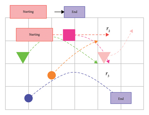
Similarly, the outflow of r2 can influence the inflow of nearby regions. Furthermore, it is worth noting that the inflow of region r2 may also impact its own outflow within the same region. There are two types of spatiotemporal correlations: semantic and spatial. While the spatial relationship reflects the region’s connectivity, the semantic relationship demonstrates the similarity of contextual traffic flow characteristics. During the morning rush hour, traffic flows mainly to different work areas. As a result, the work areas’ spatial neighbors may also have similar traffic characteristics. Currently, the effects of spatial neighbors outweigh those of semantic neighbors. At peak times in the evening, most people may travel to business areas, while few travel to work areas. Traffic patterns in similar regions are similar.
The field of statistically motivated univariate time series prediction algorithms paved the way for the first traffic forecasting methodologies. These techniques include the vector autoregressive (VAR) [12], Historical Average (HA) [13], Seasonal Autoregressive Integrated Moving Average (SARIMA) [14], and Autoregressive Integrated Moving Average (ARIMA) [15]. A fundamental prerequisite for most of these methods is the assumption that each time series has intrinsic temporal stationary. However, it is crucial to remember that these techniques, primarily based on predefined parameters not obtained from the data itself, have inherent limitations in accurately capturing the intricate spatiotemporal correlations seen in the dataset.
The motivation for using the Multi-scale Attention-Based Spatio-Temporal Graph Convolution Recurrent Network (MASTGCNet) model is its ability to accurately predict traffic patterns over long periods in a given area, particularly, in complex environments influenced by IoV systems, where real-time data and connectivity play a crucial role in traffic dynamics. This prediction can provide valuable insights for urban planners to improve road safety, traffic management, and the overall efficiency of transportation systems. The MASTGCNet hybrid model is based on a compelling rationale that aims to competently and accurately predict long-term traffic dynamics within traffic systems. This is important for city managers to make traffic flow smoother, keep roads safe, and make everything work better. Predicting traffic is useful for many things. It can help people plan their trips and know when to leave. Furthermore, the MASTGCNet paradigm opens new perspectives for integrating artificial intelligence methods in the ITS. However, the accurate and timely prediction of traffic flow statistics is a formidable and difficult undertaking.
- •
We propose a MASTGCNet. This network can carefully include data from changing graphs. This model combines spatiotemporal extraction feature mechanisms at several scales, which makes it better at processing information from a wide range of receptive regions at various hierarchical levels. Furthermore, MASTGCNet employs a resource allocation strategy within edge computing to reduce energy usage during the prediction process. The attention mechanism helps quickly determine which services are most important.
- •
We introduce a new module for extracting multiscale spatiotemporal features. This module divides input characteristics into four parallel partitions of varying dimensions, improving the capture of complex contextual information and resilience to scale changes. It also has two types of attention mechanisms that work together to understand better how space and time are connected, improving the ability to find correlations on various scales.
- •
We demonstrate the effectiveness of our proposed model through extensive experiments conducted on two different real-world traffic datasets. Our model is superior to the prevailing approaches in these empirical evaluations, demonstrating its effectiveness in traffic flow prediction.
We organize the remainder of this paper as follows: In Section 2, we expose the problem formulation. Our work methodology is briefly explained in Section 3. Section 4 describes the system architecture. Then, in Section 5, we discuss the extensive experiments conducted on two real-world traffic datasets, including empirical investigations. In Section 6, we provide the related literature. Finally, we present our concluding remarks in Section 7.
2. Problem Formulation
In this section, we formally introduce the traffic prediction problem and mathematically describe a traffic network’s concepts. Table 1 shows the summary of the most important notations.
| Notations | Description |
|---|---|
| G | Weighted graph |
| E | Set of edges |
| S | Set of nodes |
| Y : t, bt | Input and output at time t |
| A ∈ RN×N | Adjacency matrix |
| b ∈ RF | Biases |
| Wn | Reservoir weights |
| Nn | Node matrix |
| Q | Query subspace |
| V | Value subspace |
| K | Key subspace |
| X(t) | Predicted traffic flow |
| Ri | Resource allocation |
The task of predicting traffic flow can thus be viewed as a complex time series multiscale prediction problem, enhanced by incorporating auxiliary prior knowledge. In general, this involves predicting a weighted graph, typically denoted as |G| = (S, E, A), where S signifies the nodes set indicating the sources of the traffic flow and |S| = N denotes the number of nodes. At the same time, E = (i, j, wij) is a set of edges, the edge weight wij among nodes i and j represents distance, travel time, and other relevant factors. Additionally, A ∈ RN×N×T represents a spatial matrix that characterizes the internode similarities, encompassing factors, such as the distance of road network and PoI similarity. This matrix is pivotal as foundational information input for the graph convolution process. More specifically, we consider a collection of traffic data consisting of N related univariate time series denoted as Y = (X : 0, X : 1, …, X : t, …) where each constituent series X : t = (x1, t, x2, t, …, xi, t, …, XN, t) is encapsulated in a vector S ∈ RN×1 that enumerates the compilation of N sources at the discrete time instance t. Our goal is to predict upcoming values within these traffic patterns using information from historical observations.
3. Methodology
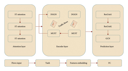
The proposed MASTGCNet model is shown in Figure 2. In this section, we first present the structure of our proposed MASTGCNet model. We then provide a detailed explanation of each component within this model.
3.1. Model Framework
The attention layer, encoder layer, and prediction layer are the three primary layers that comprise the MASTGCNet model framework. The traffic data are initially converted using a tanh activation function for stability, starting with the flow input. A feature embedding block is then used to capture complicated patterns. After that, the traffic data are analyzed through several spatiotemporal attention (ST-Attention) layers to identify geographical and temporal correlations. The encoded data are sent to the encoder layer, which manages temporal patterns and dynamic traffic variations using multiscale temporal unit (MUST) modules and Dynamic Graph Generation Networks (DGGNs). After the traffic flows are adjusted, they enter the prediction layer, where a GCN is used to capture spatial dependencies, and a sequence of ResUnits further develop deep representations. Ultimately, the prediction output is generated by a fully connected (FC) layer, which uses the processed data to represent the expected traffic flows.
3.2. Modeling Dynamic Generation Graph Network Module
Consider a graph denoted by its adjacency matrix A ∈ RN×N and the associated degree matrix D. Additionally, let θ ∈ RC×F and b ∈ RF symbolize the learning weights and biases, respectively. Here, X denotes the input, while Z denotes the output derived from the GCN layer. In the context of isolating a single node i for analysis, the operation performed by the GCN can be construed as effecting a transformation of the features of the node from an initial state, represented as Xi ∈ R1×C, to a result in the state denoted as Zi ∈ R1×F. Note that GConv represents the graph convolution operation, T1(L) denotes the first-order Chebyshev polynomial applied to the graph Laplacian matrix L, and X represents the input feature matrix. In contrast, ⊖ denotes the learnable weight parameters.
Given an individual node, denoted as i, the procedure involves extracting parameters ⊖i, unique to the i node, with a widely shared reservoir weight Wn, while exploiting the inherent node embeddings . Conceptually, this process can be seen as a mechanism for acquiring node-specific patterns by identifying specific patterns inherent in a broader collection of prospective patterns derived from all the traffic sequences.
3.3. Modeling Dynamic Multiscale Spatiotemporal Feature Unit
3.4. Modeling Attention-Based Spatiotemporal Module
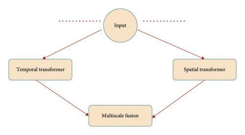
To ensure robustness, we use a residual connection W′ = W + Z during training phase. The resulting output of every node is denoted as Y′ = U + W′, and this process ultimately leads to the parallelization of outputs across all nodes, yielding .
To extend the scope of time series forecasting for extended prediction horizons, we intelligently capture bidirectional temporal dependencies over an extended period. This is accomplished within the structure of a sliding window, operating at each discrete temporal instance. The hierarchical architecture of the TT effectively captures complex dependencies across multiple layers, thereby enabling the prediction of long sequences without sacrificing computational efficiency by increasing the parameter T. In contrast, RNN-based methods face vanishing gradients, while models based on convolutional methods require an explicit specification of an expanding convolutional layer concerning the parameter T.
3.5. Multiscale Feature Extraction Unit
4. System Architecture
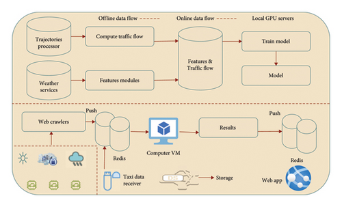
In Figure 4, we illustrate the architecture of our system, which comprises three primary components: local GPU servers, the Cloud, and users (e.g., through websites). This setup facilitates both offline and online data flows. The local GPU servers store historical observations, such as taxi trajectories and meteorological data. The Cloud receives real-time data, including real-time traffic information (such as trajectories within specific intervals) and meteorological updates. The suggested energy-efficient resource allocation plan for the edge-cloud architecture is the main topic of Section 4. The attention mechanism determines the importance of prediction tasks, and the method dynamically allocates computational resources accordingly. This enables the system to optimize energy consumption by prioritizing high-demand operations, such as busy traffic regions or crucial crossings, while allocating fewer resources to less crucial jobs. While the cloud handles more complicated activities, the edge servers manage time-sensitive predictions to reduce latency. The precise resource allocation algorithm, the metrics used to assess resource efficiency, and the experimental findings that show how well this strategy works to lower energy consumption while preserving high prediction accuracy are just a few of the extra details we will cover in this section. Users interact with the system to access both inflow and outflow data.
4.1. Efficient Cloud-Based Traffic Flow Analysis
In the context of edge-cloud computing, the prediction model performance is optimized in large part by the energy-efficient resource allocation. Through the distribution of computational activities between edge servers and the cloud, the edge-cloud architecture guarantees low latency and energy-efficient processing. By prioritizing tasks using the attention mechanism, the resource allocation technique enables the system to distribute computational resources and reduce energy usage dynamically. This method guarantees timely and effective traffic projections, particularly in smart city settings. This dual focus is reflected in the title, highlighting energy efficiency and traffic prediction, ensuring that both are well represented in the final solution.
We leverage the Azure platform as a service (PaaS) for our system, ensuring efficient resource allocation and task assignment, particularly when processing the vast amounts of data generated by IoV systems. Table 2 offers a comprehensive breakdown of the Azure resources utilized in our setup, meticulously optimizing for both performance and cost-effectiveness. In forecasting crowd flows for the near future, we prioritize energy-efficient resource allocation by employing a VM known as the A2 standard in Azure. With its 2 cores and 3.5 GB memory, this VM strikes a balance between computational power and energy consumption. To efficiently handle potential heavy traffic from numerous users, especially the data influx from IoV systems, we employ an energy-efficient task assignment strategy by hosting both the website and web service on an App Service. Furthermore, to minimize energy consumption while ensuring data accessibility, historical data are stored on local servers, while a 6-GB Redis cache efficiently caches real-time trajectories from the past half-hour, crowd flow data, extracted features from the past 2 days, and inferred results.
| Azure service | Configuration | Prices |
|---|---|---|
| Virtual machine | Standard A2 (2 cores, 3.5 GB memory) | $0.120/h |
| App service | Shared plan, A2 standard, 2 cores | $0.400/h |
| Redis cache | 6 GB, PI premium | $0.55/h |
4.2. Local GPU Servers
While many tasks can be performed on the cloud, GPU services are unavailable in certain regions such as China. Implementing energy-efficient resource allocation and task assignment strategies is essential in optimizing cloud-based operations. Additionally, there are expenses associated with other edge computing services, such as storage and I/O bandwidth. Therefore, cost-saving measures are crucial for a research prototype. Moreover, transferring large volumes of data from local servers to the cloud is time-consuming due to limited network bandwidth. Energy-efficient data transfer protocols and task prioritization algorithms can help mitigate delays caused by data migration. For example, historical trajectories can span hundreds of gigabytes or even terabytes, resulting in significant delays when copying data from local servers to the cloud. Efficient compression algorithms and prioritization mechanisms can be employed to streamline the transfer process and minimize energy consumption.
- •
Transforming trajectories into inflow/outflow data involves utilizing extensive historical trajectory datasets and employing a computation module to derive crowd flow information, which is subsequently stored locally.
- •
Gathering features from external sources entails initially aggregating external datasets from various data repositories, such as weather and holiday events. These datasets are then processed through a feature extraction module to generate continuous or discrete features stored locally for further analysis and utilization.
- •
To train our predictive model, we utilize the generated crowd flows and external features through our proposed MASTGCNet framework. The trained model is then uploaded to the cloud. Since the dynamic crowd flows and features are stored in Azure Storage, we synchronize the online data with our local servers before each training session. This approach allows us to experiment with new ideas, such as retraining the model, while significantly reducing costs for a research prototype.
4.3. Training Process
Algorithm 1 describes the training procedure of MASTGCNet. Backpropagation is used randomly to initialize and optimize the trainable parameters based on MASTGCNet. Backpropagation minimizes the loss function of our proposed model using the stochastic gradient method. We implement the dropout strategy approach to increase the overall effectiveness of our method. Algorithm 2 aims to optimize resource allocation for energy-efficient traffic flow prediction. During training, it iteratively adjusts the allocation of computational resources based on the processing time, prediction accuracy, and energy consumption. The optimization process involves fine-tuning the model and resource distribution to meet the constraints of maximum allowable processing time; minimum required prediction accuracy, and maximum available resources, ensuring that the model achieves high accuracy with minimal energy usage.
-
Algorithm 1: The MASTGCNet algorithm.
-
Input: Historical observations: {Xt|t = 1, 2, …, T}; The spatial graph Z: {Nt|t = 1, 2, …, n}; Pre-defined graph {|G| = (S, E, A)};
-
Output: Learned MASTGCNet Model
- 1.
D ⟵ 0;
- 2.
for all accessible time interval t (2 ≤ t ≤ n) do
- 3.
Z = [b + X(1 + D(−1/2)AD(−1/2))];
- 4.
D(−1/2)AD(−1/2) = tanh(ReLU(NNT));
- 5.
Z = b + X ⊖ (I + tanh(ReLU(NNT)));
- 6.
Put a training instance (Xt) into D;
- 7.
end for
- 8.
// Training the model;
- 9.
initialize learnable parameters ⊖ in MASTGCNet;
- 10.
repeat
- 11.
randomly chose batch of instances Dbatch from D;
- 12.
calculate ⊖ by reducing the objective with Db;
- 13.
until model criteria met;
- 14.
return MASTGCNet model
-
Algorithm 2: Energy-efficient resource allocation for traffic flow prediction.
-
Input: Traffic data , Weather data , Maximum allowable processing time Tmax, Minimum required prediction accuracy Pmin, Maximum available resources
-
Output: Optimized resource allocation , Predicted traffic flow
- 1.
Initialize resource allocation ;
- 2.
Initialize model ;
- 3.
while not converged do
- 4.
Compute traffic features ;
- 5.
Compute weather features ;
- 6.
Compute processing time ;
- 7.
Compute prediction accuracy ;
- 8.
ifTproc > Tmaxthen
- 9.
Adjust resources to reduce processing time: ;
- 10.
end if
- 11.
ifAccuracy < Pminthen
- 12.
Adjust model or resources to improve accuracy: ;
- 13.
end if
- 14.
Update total energy consumption ;
- 15.
ifthen
- 16.
Adjust resources to minimize energy consumption: ;
- 17.
end if
- 18.
end while
- 19.
Compute final predicted traffic flow ;
- 20.
return, .
5. Experiments and Performance Analysis
We have implemented and empirically evaluated the MASTGCNet model using two large traffic datasets, BikeNYC and TaxiBJ. We first talked about the datasets we used, how we set some parameters, and how we measured how well the model worked. Next, we discussed other models recently proposed for traffic prediction.
5.1. Experiment Setup and Datasets
We use a Linux server with numerous software, as defined later in Section 5.3, and hardware described in Table 3.
| Component | Specification |
|---|---|
| CPU | 8 Intel (R) Core (TM) Xeon (R) CPU E5-2680; v4 @3.80 GHz |
| GPUs | 4 NVIDIA P100 |
| cuDNN version | 8.0 |
| CUDA version | 8.0 |
| RAM | 256 GB |
- •
TaxiBJ: The city of Beijing provided the taxi trajectory data for this dataset over 16 months: from July 1, 2013, to October 30, 2013, from March 1, 2014, to June 30, 2014, from March 1, 2015, to June 30, 2015, and from November 1, 2015, to April 10, 2016. The dataset contains over 35,000+ taxi trajectories, effectively capturing urban traffic flows in Beijing. We partition the data, using a subset for training and reserving the most recent 4-week period for data testing.
- •
BikeNYC: The BikeNYC dataset was generated from February 5, 2014, to August 29, 2014. This dataset contains 6900 traffic flow maps, with dimensions of 16 × 8 and a temporal resolution of 1 hour. It includes extensive bicycle-related information, including attributes such as trip distance, start and end times, and origin and destination station identifiers. We refer to the last 10 days of the dataset as the test set for evaluation purposes and the previous days as the training set.
| Datasets | TaxiBJ | BikeNYC |
|---|---|---|
| Urban | Beijing | New York |
| Format of data | Taxi GPS | Rent bike |
| Time span | July 1, 2013–October 30, 2013 | February 5, 2014–August 29, 2014 |
| March 1, 2014–June 30, 2014 | ||
| March 1, 2015–June 30, 2015 | ||
| November 1, 2015–April 10, 2016 | ||
| Period | 30 min | 1 h |
| Taxis and bikes | 35,000+ taxis | 6900+ bikes |
| Map size | 32 × 32 | 16 × 8 |
5.2. Compared Methods
To measure the overall performance of our approach, we conducted a comprehensive comparative assessment by comparing the MASTGCNet to prominent, well-known models and state-of-the-art methods in the field, including the following:
5.2.1. Conventional Time-Series-Based Models
5.2.2. Deep Learning-Based Models
- •
FC-long short-term memory (LSTM) [21]: It is essentially a fusion of the codec and LSTM models, where each section of the encoder and decoder consists of a certain number of recurrent layers. It is important to note that these recurrent layers contain a defined number of LSTM units. Furthermore, the FC-LSTM model integrates both approaches to predict the result.
- •
GRU-ED [22]: A model using an encoder–decoder framework based on GRU was used to perform the machine translation task.
- •
STGCN: This model contains a distinct element called a spatiotemporal block. These blocks are stacked in multiple layers, denoted as k layers, within the model’s core. This configuration greatly assists the model in achieving convergence. Ultimately, at both the beginning and end of the process, a 1 × 1 convolutional layer is employed by the model to aggregate, integrate, and predict various features.
- •
Graph WaveNet [23]: In this study, the authors offer Graph WaveNet, a unique graph neural network architecture, for spatial–temporal graph-based modeling.
- •
RPConvformer [24]: The upgraded components of a novel framework named RPConvformer are 1D causal convolutional sequence embedding and relative position encoding.
- •
ST-ResNet [25]: The ST-ResNet method used a residual-based network to predict urban traffic flows throughout the city. This approach has demonstrated superior performance compared to alternative methods.
- •
MST3D [26]: This model predicts the vehicle flow throughout the city, the MST3D model employs 3D CNN models to jointly capture multiple spatiotemporal dependencies.
- •
MASTGCNet: In this work, we combine the GCN and GRU, this framework effectively extracting dynamic features of spatiotemporal from node properties. MASTGCNet implements a resource allocation strategy aimed at minimizing energy consumption during the prediction process.
5.3. Implementation Details and Evaluation Metrics
5.3.1. Preprocessing
In the case of the TaxiBJ dataset, the urban area was partitioned into discrete grid regions measuring 32 × 32 units, with each temporal segment corresponding to a duration of 30 min. In a parallel manner, for the BikeNYC dataset, we adopted a grid structure comprising dimensions of 16 × 8 to represent the city map, with each temporal interval set at 1 hour. To make the traffic flows comparable, we scaled them between −1 and 1 using a method called min–max normalization. After the prediction, we adjusted the values to match our research’s usual output and compared them with the actual values. The hyperparameter settings are briefly described in Table 5.
| Hyperparameter description | Value or range |
|---|---|
| Keras | 2.2.4 |
| TensorFlow | 1.13.1 |
| Python | 3.6 |
| Learning rate | 0.001 |
| Optimization algorithm | Adam |
| Number of epochs | 200 |
| Dropout rate | 0.25 |
| Batch size | 64 |
| Early stopping patience | 15 |
5.3.2. Evaluation Metrics
5.4. Experiment Results and Analysis
Using the setup and settings mentioned above, we compared how well our MASTGCNet model performed against other competing methods on two real-world datasets: BikeNYC and TaxiBJ. The results are shown in Figures 5 and 6, respectively. The MASTGCNet stands out by achieving the lowest MAPE and RMSE values among all methods, demonstrating its superior performance. Specifically, for BikeNYC, the RMSE is about 4.02, and the MAPE is 18.75%. Similarly, for TaxiBJ, the MAPE is about 14.09 and the RMSE is about 12.43%, respectively. This indicates that our added attention and multiscale feature framework effectively improve the performance of the proposed model. We also use standard deviation, which serves as a valuable metric to assess the consistency and stability of traffic patterns, aiding in anomaly detection, model evaluation, and informed traffic management decisions.
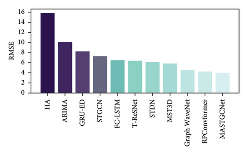
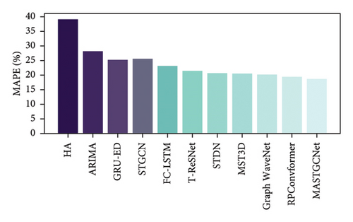
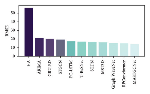
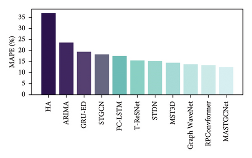
We compared the average results of our method with other methods on two datasets, TaxiBJ and BikeNYC. The results are shown in Table 6. We calculated the average performance for each model by running it 10 times. Table 6 clearly shows that our proposed MASTGCNet model outperforms the other models regarding effectiveness and prediction accuracy. These results highlight the value of our model in understanding the spatiotemporal relationships in predicting traffic flows.
| Methods | BikeNYC | TaxiBJ | ||
|---|---|---|---|---|
| RMSE | MAPE (%) | RMSE | MAPE (%) | |
| HA | 15.80 | 38.99 | 55.99 | 36.89 |
| ARIMA | 10.10 | 27.99 | 20.99 | 23.45 |
| GRU-ED | 8.23 | 25.09 | 20.18 | 19.35 |
| STGCN | 7.32 | 25.39 | 19.18 | 18.21 |
| FC-LSTM | 6.49 | 22.98 | 17.32 | 17.42 |
| ST-ResNet | 6.34 | 21.31 | 16.89 | 15.39 |
| STDN | 6.20 | 20.65 | 16.50 | 15.15 |
| MST3D | 5.81 | 20.39 | 15.90 | 14.41 |
| Graph WaveNet | 4.52 | 20.15 | 15.26 | 13.75 |
| RPConvformer | 4.27 | 19.34 | 14.95 | 13.24 |
| Our (MASTGCNet) | 4.02 | 18.65 | 14.09 | 12.43 |
Our MASTGCNet method significantly reduces prediction errors during model training when combined with the spatiotemporal GCN. This demonstrates the adaptability of our method for urban traffic flow prediction. The efficiency of the MASTGCNet model exhibits consistent enhancement, particularly within the domain of long-term traffic flow prediction. In particular, traditional methods, such as ARIMA and HA, struggle to produce highly accurate forecasts, highlighting the limitations of approaches that ignore dynamic spatiotemporal dependencies and focus solely on historical statistical relationships. ARIMA focuses on modeling univariate time series and does not incorporate spatiotemporal correlations between different regions. This limitation prevents the model from exploiting important network structure and road system insights. Incorporating spatial correlations improves regression models such as FC-LSTM and GRU-ED, but they can still not capture the complex dynamic nonlinear spatial and temporal dependencies. The FC-LSTM cannot typically explicitly capture the spatial dependencies in traffic data, which can be crucial for accurate traffic flow prediction in scenarios where road networks play a significant role. Furthermore, our model outperforms the ST-ResNet and MST3D models. The ST-ResNet residual structure is limited in capturing the highly nonlinear relationships in complex traffic dynamics. Similarly, the MS3TD model has a higher number of hyperparameters that require thorough tuning to achieve optimal performance. Insufficient tuning can lead to suboptimal results.
The current methods struggle to predict traffic flow prediction in a given area accurately. Existing approaches such as CNN, RNN, and LSTM manually extract information from images, which reduces prediction accuracy. We need updated methods that automatically gather information using techniques such as the GCN and attention modules. These approaches dynamically gather information from models, improving prediction accuracy while saving time and resources. If we look at the figures (Figures 5 and 6) and compare them with existing methods, it is clear that existing models do not perform as well as our proposed model. Our proposed model achieves better accuracy regarding time, cost, and reliability. It is more reliable and adaptable because it dynamically processes information instead of manually manipulating images. We also combined our model with spatiotemporal techniques to improve training and reduce prediction errors. This combination also speeds up the training time, showing that our model can work well in different situations.
Our model combines the spatiotemporal GCN network to make training more accurate and reduce prediction errors. We tested our model against existing long-term traffic flow prediction methods and found that it performed much better. The existing models used CNN, LSTM, or RNN separately with manual data extraction, which made training longer instead of more efficient. To improve prediction accuracy, we need to extract features from the traffic flow data dynamically. Our model, which uses neural networks such as GCN and RNN with an attention mechanism, allows us to easily estimate traffic flow in a city, including the number of people entering and leaving. This allows us to reduce training time, make predictions more accurate, and save time and cost.
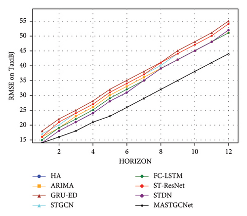
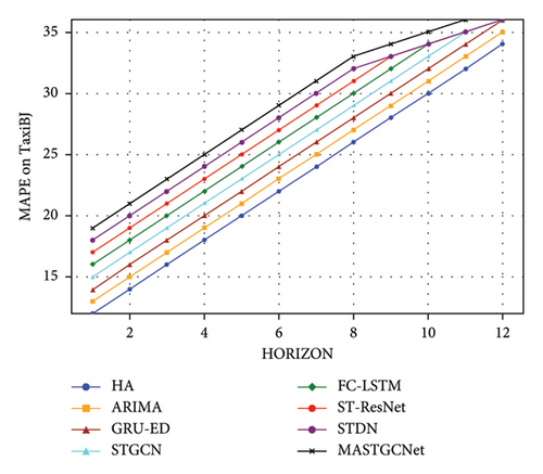
In addition, Figure 7 illustrates the prediction performance of various models across different horizons on the TaxiBJ dataset. Our proposed model consistently performs best across all prediction horizons and evaluation metrics, demonstrating its superior ability to capture heterogeneous spatiotemporal dependencies. While STDN shows comparable performance to our model in the first three horizons, its accuracy declines as the prediction horizon increases. This indicates that our model is robust to changes in prediction horizons and underscores the effectiveness of the temporal dependence extraction units in MASTGCNet.
5.5. Results of Different MASTGCNet Variants
To validate the effectiveness of the MASTGCNet method, we conducted a thorough empirical assessment, examining different variants while maintaining consistent experimental setups. Our evaluation focused on three key aspects: (i) assessing the impact of model depth, (ii) analyzing the effects of varying kernel and filter numbers, and (iii) investigating computational complexities, including prediction and training times. The subsequent sections delve into a detailed discussion of these findings, shedding light on our proposed algorithm’s performance and computational considerations.
5.5.1. Impact of Depth Model
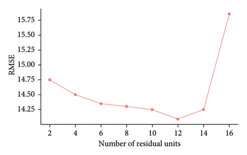
We conducted an extensive empirical experiment with nine different variations of the MASTGCNet model, each characterized by different depths. We aim to achieve deeper insights into the effectiveness of different depths within the MASTGCNet model. The experimental results are shown in Figure 8. Focusing specifically on the TaxiBJ dataset, Figure 8 provides a detailed visualization of the impact of model depth. Our results show a compelling relationship between the number of residual units representing network depth and the RMSE metric. As we progressively increase the depth of the network by increasing the number of residual units, we observe an initial increase in RMSE, followed by a subsequent increase in RMSE. This trend indicates that deeper networks yield better results. Nevertheless, it is crucial to note that as the number of residual units exceeds a certain threshold, such as ≥ 12, the training process becomes more complex, and the risk of overfitting increases.
5.5.2. Impact of Filter Numbers and Filter Sizes
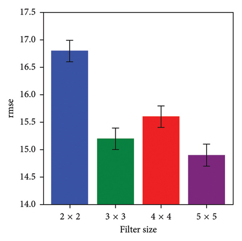
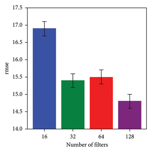
We have extensively explored different dataset training configurations to optimize filter size selection. Achieving precise prediction accuracy depends on the careful selection of filter size. As shown in Figure 9(b), we observed the profound impact of filter size on the performance of the MASTGCNet methodology. To carefully observe and illustrate the effects of filter size, we systematically adjusted the filter dimensions, ranging from 2 × 2 to 5 × 5. Figure 9(b) shows a noteworthy trend: an increase in kernel size corresponds to a decrease in the RMSE metric. In addition, as shown in Figure 9(a), the use of larger filter sizes consistently yields significantly better results than the use of smaller filter sizes. This pattern is consistent with our observations regarding filter size and number of filters.
5.6. The Convergence of MASTGCNet Model
Figure 10 illustrates the loss curve of the MASTGCNet model on two real datasets, depicting the training and validation RMSE during the experiment. In Figure 10(a), on the BikeNYC dataset, the RMSE for both the training and validation sets gradually decreases with increased training iterations. Around Iteration 65, the RMSE for both sets stabilizes. In Figure 10(b), for the TaxiBJ dataset, the RMSE for both the training and validation sets also decreases with increasing iterations, reaching stability around Iteration 128.
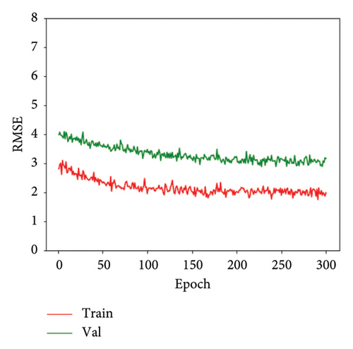
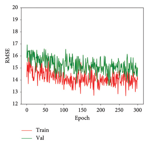
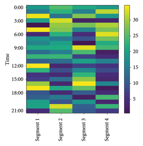
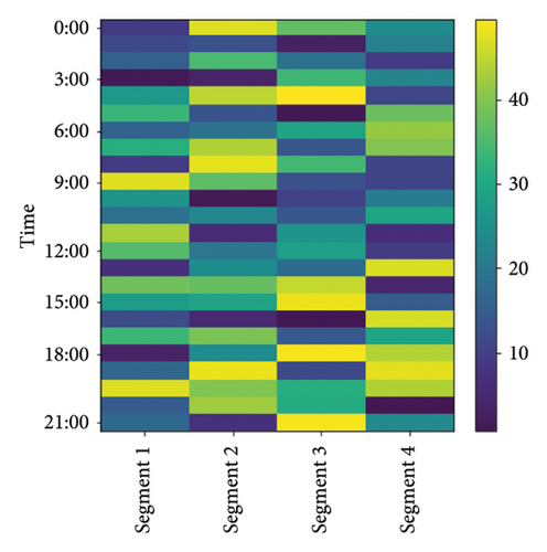
Figure 11 illustrates that the traffic state matrix varies across different time segments. Initially, the feature matrix before training appears random and unstructured. However, after training, the feature matrix displays distinct temporal patterns similar to the traffic state matrix. This demonstrates that the model successfully learns and abstracts temporal features for prediction.

5.7. Model Efficiency
Subsequently, we conduct a thorough investigation of the performance of our proposed model works both in predicting outcomes and in the training phase, taking into account the response time. We have summarized the results in Table 7. One thing that immediately stands out is that our MASTGCNet model performs better than the STDN and MST3D models in both the training and prediction phases. It is worth noting that the STDN method takes the longest time for both training and prediction. This is because STDN uses certain computations called local CNNs to make predictions, and it also has to go through the entire region using a sliding window. For example, if we work with a dataset like BikeNYC, predicting values for the entire region requires performing a certain computation 16 × 8 times. On the BikeNYC dataset, our MASTGCNet model significantly outperforms the ST-ResNet approach. This happens mainly because our MASTGCNet method combines two techniques, GCN and GRU, based on GCNs. We see a similar trend on the TaxiBJ dataset. Our MASTGCNet model outperforms both the MST3D and STDN baselines in terms of both prediction speed and training speed. These results demonstrate the advantages of our model.
| Methods | BikeNYC | TaxiBJ | ||
|---|---|---|---|---|
| Training time (s/epoch) | Prediction time (s) (%) | Training time (s/epoch) | Prediction time (s) | |
| STDN | 18,973 | 88.7 | 369,601 | 207.4% |
| MST3D | 126 | 0.23 | 5902 | 2.74% |
| Our (MASTGCNet) | 116 | 0.08 | 4845 | 2.57 |
The time and space complexities of Algorithm 1 are closely related to key parameters, mainly the amount of available historical information and the number of features. In particular, the complexities depend on two crucial factors: the training time, denoted by m, which is the time required to form the dataset D, and the learning time, denoted by n, which characterizes the time required to acquire knowledge within the model while keeping the computational overhead for θ constant. It is important to understand that the algorithm’s performance shows different behaviors under different circumstances. In the best-case scenario, the algorithm exhibits a time complexity denoted by ω(m + n). In this case, the computational cost escalates linearly with both training and learning times. This scenario represents an optimal match of algorithm efficiency with available computational resources, culminating in a favorable performance profile. Conversely, the worst-case scenario reveals a potentially significant time complexity that can rise to O((mn)(m + n)) and further simplifies to O(m2n + n2m). This particular scenario depends on the number of observations and the dimensionality of the features. This worst-case behavior serves as a stark reminder of the paramount importance of carefully considering resource constraints and dataset characteristics when implementing Algorithm 1.
6. Related Works
In this section, we emphasize how we use deep learning to understand the spatiotemporal correlation for traffic prediction. We also look closer at the concept of attention, which plays an important role in our model.
6.1. Traffic Flow Prediction
In the field of traffic prediction, the incorporation of predictive spatial information is emerging as a key factor. Modern methods using convolution neural networks (CNNs) [27, 28] for traffic flow mapping often rely on grid-based map segmentation. However, the inherent regularity of grid-based data limits their ability to represent complex spatial information effectively. Reference [29] proposed a unique multitask spatiotemporal network for highway traffic flow prediction (MT-STNet) that combines multitask learning, generative inference system, and encoder–decoder structure. References [30, 31] (DCRNN) innovatively presented a diffusion convolution RNN based on distance graphs. Their approach incorporates bidirectional random walks on the graph to capture spatial dependencies.
However, the establishment of spatial topology in these methods through predefined adjacency matrices remains static and limited in nature, with inherent limitations in encapsulating the complex characteristics of complex road networks. Existing methods based on predefined graph structures face significant challenges. First, predefined graph constructs struggle with sparsity issues. Sparsity, which is particularly evident in large graphs, manifests itself in the adjacency matrix, leading to computationally inefficient operations and may fail to encapsulate the totality of spatial dependencies comprehensively. This, in turn, can potentially undermine the accuracy of the model [32]. A secondary concern revolves around the inflexible nature of predefined adjacency matrices, which makes them ill-suited for accommodating dynamic graphs or graphs characterized by recurrent structural changes [33].
In conjunction with the previous discourse on the construction of spatial topology, the strategic modeling of spatial and temporal dependencies emerges as a key factor in traffic prediction. Capturing temporal dependencies requires recourse to rRNNs and their diversification, which are expertly tailored to sequential data with intrinsic capabilities to capture temporal correlations of a temporal nature [34, 35]. The recurrent nature of RNN operations provides increased model flexibility. In Ref. [36], this paper proposes a unique deep learning approach to improve traffic volume forecasting accuracy by addressing these shortcomings. In order to create synthetic data or synthetic traffic volume, a new spatiotemporal dependencies generative adversarial network are first proposed.
In contrast to the more complicated LSTM [37], GRU advocates a simpler and more trainable architecture. Gaining prominence for their effectiveness and versatility, attention mechanisms [38] have found widespread application in various domains. These mechanisms automatically focus on central information extracted from historical input data. Graph attention networks (GANs) [5] have made significant progress in traffic prediction by constructing spatial models. STSGCN [39] introduces a novel concept by devising a synchronized GCN model for spatial and temporal aspects. These modules adeptly capture correlations across space and time. In Ref. [40], to further improve the traffic flow forecasting outcomes, the researchers offer a unique spatial–temporal gated hybrid transformer network (STGHTN), which utilizes global features by transformer and local information from temporal gated convolution and spatial gated graph convolution, respectively. We advised the MASTGCNet model, which combines the GCN with the attention unit to collectively incorporate both the features of spatiotemporal traffic flow, drawing inspiration from previous research as discussed above.
6.2. Attention Mechanism
The attention mechanism has become an important tool in various tasks such as language translation and image recognition, helping to decide which parts are most important to focus on Ref. [41]. This mechanism uses a process where a question and a set of key-value pairs create an output. The output is a mixture of the values, with the importance of each value determined using a compatibility function between the question and its key. Attention mechanisms are generally used in conjunction with convolutional or recurrent networks. In Ref. [42], they present an attention-based spatiotemporal graph attention network (ASTGAT) model for network degradation and oversmoothing issues. In Ref. [43], the model relies on attention to see connections between input and output. Recently, attention mechanisms have also been used in graph neural networks. In Ref. [44], they introduced gated attention networks for graph learning. In Ref. [45], a brand-new GCN dubbed TFM-GCAM incorporates attention mechanisms to better capture nodes’ dynamic properties and spatial–temporal attributes.
7. Conclusions and Future Work
In this paper, we proposed a new approach to traffic flow prediction using a deep learning model called MASTGCNet. To address the complexities of traffic, we introduced a dynamic graph generation component and a spatiotemporal multiscale feature extraction component to the standard GCNs. These components help the model learn specific patterns for each point and understand relationships at different levels of detail in the data. We performed experiments using baseline techniques on two extensive traffic flow datasets to confirm the efficiency of our MASTGCNet model. The experimental outcomes affirm the MASTGCNet model’s performance and the proposed MUST module. MASTGCNet implements a resource allocation strategy within edge computing to minimize energy consumption during prediction.
In the future, we aim to increase the model simplicity to facilitate its seamless application to related tasks. This approach is intended to strengthen the model’s performance and capacity for broader applicability. In addition, we plan to improve our model by integrating external factors, such as unexpected events and weather conditions, to increase its predictive accuracy.
Conflicts of Interest
The authors declare no conflicts of interest.
Author Contributions
A.A.: conceptualization, software development, and writing – original draft. I.U.: writing – original draft and visualization. S.K.S.: writing – review and editing and revision. A.S.: visualization and revisions. W.J.: visualization, revisions, and writing. H.I.S.: writing – review and revisions. X.B.: conceptualization, software development, writing – original draft, and revisions.
Funding
This work was supported in part by the National Natural Science Foundation of China under Grants 62373255 and 62173234, in part by the Natural Science Foundation of Guangdong Province under Grant 2024A1515011204, in part by the Shenzhen Natural Science Fund through the Stable Support Plan Program under Grant 20220809175803001, and in part by the Open Fund of National Engineering Laboratory for Big Data System Computing Technology under Grant SZU-BDSC-OF2024-15.
Acknowledgments
This work was supported in part by the National Natural Science Foundation of China under Grants 62373255 and 62173234, in part by the Natural Science Foundation of Guangdong Province under Grant 2024A1515011204, in part by the Shenzhen Natural Science Fund through the Stable Support Plan Program under Grant 20220809175803001, and in part by the Open Fund of National Engineering Laboratory for Big Data System Computing Technology under Grant SZU-BDSC-OF2024-15.
Open Research
Data Availability Statement
The data that support the findings of this study are available from the corresponding author upon reasonable request.


