Exploring Batch Normalization’s Impact on Dense Layers of Multiclass and Multilabel Classifiers
Abstract
Leveraging batch normalization (BN) is crucial for deep learning for quick and precise identification of objects. It is a commonly used approach to reduce the variation of input distribution using BN. However, the complex parameters computed at the classifier layer of convolutional neural network (CNN) are the reason for model overfitting and consumption of long training time. This study is proposed to make a comparative analysis of models’ performances on multiclass and multilabel classifiers with and without BN at dense layers of CNN. Consequently, for both classifications, BN layers are incorporated at the fully connected layer of CNN. To build a model, we used datasets of medical plant leaves, potato leaves, and fashion images. The pretrained models such as Mobile Net, VGG16, and Inception Net are customized (tuned) using the transfer learning technique. We made adjustments to training and model hyperparameters, including batch size, number of layers, learning rate, number of epochs, and optimizers. After several experiments on the three models, we observed that the best way to improve the model’s accuracy is by applying BN at the CNN’s dense layer. BN improved the performances of the models on both multiclass and multilabel classifications. This improvement has more significant change in the multilabel classification. Hence, using medicinal plant dataset, the model achieved accuracy of 93% and 83% for multilabel with and without BN, respectively, while achieving 99.2% and 99% for multiclass classification. The experiment also proved that the effectiveness of BN is affected on type datasets, depth of CNN, and batch sizes.
1. Introduction
A deep neural network is the building block of the deep learning algorithm. Deep learning uses a convolutional neural network (CNN) for object detection and classification of images constituting its main functions. CNN has made it accessible to the deep learning model to automatically extract features from images during training. The convolutional network feature extractor is made up of particular types of neural networks, where the training process determines the weights for classification [1]. Binary, multiclass, and multilabel classifications frequently encountered difficulties with classification. Two subcategories of single-label classification are traditional binary and multiclass classifications [2]. All classification approaches were achieved by deep learning which is widely used to solve a complicated task. To tackle problems related to the actual world, such as satellite image classification, bioinformatics, audio recognition, machine translation, and medicinal plant identification, a comprehensive study was carried out [3–5].
To apply multilabel classification, we used the problem transform method with the binary relevance technique by which the model performs binary classifier for each class (label) [2, 6]. Multilabel classification is a more difficult task than multiclass because both the input images and output label spaces are more complex [7]. The probability of each target label in multilabel classification is determined using a sigmoid classifier. Dependability across classes is the primary distinction between multilabel and multiclass classification. In multiclass classification, if there are five target classes (nodes), a target node (output neuron) with a greater probability than the other four classes (nodes) can be considered the winner. The probability of each target class is determined using a softmax classifier. So, the result of given input data depends on the probability of other remaining target labels (output nodes). Unlike multiclass, in multilabel approach, every kind of input data has its own multiple target labels. Multilabel classification can be defined as the problem of assigning multiple labels to each given instance [8]. So, the result should be calculated independently using a sigmoid classifier [9], in which its value is either 0 or 1. Figure 1 elaborates more. At the left side, input image is classified as both bark and leaf which is a multilabel output at a time. While looking to the right side, it is a multiclass classification task with the SoftMax layer by which a class (category) with a higher probability value is selected at a time.

CNN computes in a convolutional process using an image pixel as input for both multiclass and multilabel classifications. Due to the need for smaller training steps (learning rates), this leads to the training step to take an extended period of time or slow down [9]. Therefore, the correct solution is using high learning rate. However, a high learning rate causes the gradients to expand or vanish and become stacked in local minima [9]. The change in the distributions of inputs to the convolutional layers is also the main challenge of the deep learning model because the layers need to continuously adapt to the new distribution [10]. This indicates that the input that the network has learned from onward is different from the modified input distribution to the CNN. We characterize this particular problem as an internal covariate shift [11, 12]. The test dataset for the covariant shift model could be another novel input distribution [12]. In this scenario, the training process slows down and it takes some time for it to converge to global minima. However, other factors may contribute to training time consumption beyond modifications to input distribution. It also matters what type of convolution by which the model is developed? What optimizer is used? And how big and high-quality the dataset is?
Many scholars tried to solve the covariant shift problem by normalizing layer inputs. Input normalization is computed by standardizing each mini batch input using its mean and standard deviation in training data. This standardization technique is batch normalization (BN). BN is a popular method for fastening the training of deep learning models. The technique also enabled us to use higher learning rate–maintained nonlinearities in the feed forward process. BN is also a technique to normalize activations in hidden layers of deep neural networks [9].
- •
Input distributions are changed in each hidden layer. So, there is a lot of input feature modification.
- •
A small change at the output of first hidden layer causes huge change at the last hidden layer.
- •
The first mini batch data pass through feedforward computation, and after computing the error, CNN backpropagates to update the weight. The next batch is multiplied by the updated weight. Hence, there will be change in input distribution at each hidden layer and fully connected (FC) layer.
Extensive researchers explored that change in distribution of input data was the cause for internal covariant shift. This change of input distribution can occur due to updated weight values in each hidden layer during backpropagation because each kind of input batch data is multiplied by the updated weights for the next iterations (epochs). Hence, change in weights at the previous layer changes the input distribution at the current layer and pushes the current layer to learn from scratch. The internal covariant shift occurs in both hidden (training) layer of CNN and FC layer. Internal covariant shift not only slows down the training time but also consumes testing time. Hence, BN should be applied at the classifier (FC) layer of CNN.
- •
We investigated the importance of adding BN at the FC layer for enhancing the performance of the deep learning model particularly in the models that compute complex and interdependent outputs such as multilabel classification.
- •
Accordingly, our experiment proved that adding BN at FC layer of CNN improved the robustness of a multilabel classifiers.
- •
A comprehensive comparison was conducted on three multilabel and multiclass classifier models using three different datasets. Hence, we ensured that leveraging BN at FC layer of multilabel classifier is advantageous than multiclass classifier.
- •
The study proved that the effectiveness of BN also depends on the batch size, type of dataset, and depth of CNN. So, it is important leveraging BN at the FC layer of CNN to train the model using an unbalanced dataset and larger batch size and learning rate.
This paper is organized as follows. Section 2 presents a detailed description of the related work, including the gaps and measures taken. In Section 3, a detailed description of the proposed methods and the dataset analyzed in this study is given. In Section 4, the experimental findings and analysis are provided. Finally, we presented the concluding remarks.
2. Related Works
This section provides a concise description of many techniques that have been done previously. Following that, many scholars began expressing interest in this field with the advent of public domain, and significant effort and advancement have been made.
It is computationally expensive to train deep neural network. Many researchers tried to solve the problems by using data normalization. Schilling [13] applied layer normalization on recurrent neural network by computing the mean and variance from all of the summed inputs to the neurons in a layer on a single training case. Ba, Kiros, and Hinton [14] used BN to minimize the divergence of loss and inconsistent growth of activation function with network depth, which limits possible learning rates. As stated by Bjorck et al. [15], BN makes the gradients more predictive and allows for the use of larger learning rates and faster network convergence. BN can be improved by normalizing with respect to multiple mean and standard deviations associated with different modes of variation in the underlying data distribution [16]. The correct normalization helps the training of CNN models and improves the model performance with a large margin [17].
Wang et al. [18] used deep learning technique and stacked autoencoders (SAEs) with the addition of BN in feature learning layer of DNNs to achieve a fast intelligent fault diagnosis of machines from bearing and gearbox datasets. Wang et al. [19] proposed group normalization to improve the performance of a model using visual question answering, few-shot learning, and conditional image generation. In. Michalski [20] BN significantly improved the accuracy of the classification model designed by DNN to recognize the Patik pattern. Nurhaida et al. [21] leveraged BN before the output layer of the CNN that reduced the vanishing gradient and improved the performance of the model. Thakkar, Tewary, and Chakraborty [22] demonstrated the importance of BN by conducting comparative analysis on Dense Net, VGG, Residual Network, and Inception (v3) with CIFAR-10 dataset. Liu et al. [23] leveraged batch normalization in the CNN and inception residual (BIR) network modules to detect and classify Android malware from CICAndMal2017 which is a publicly available network traffic dataset. Liu et al. [24] made a comparative analysis on the accuracy of facial expression classifier models with and without layer normalization. They proved that the model with BN has reduced overfitting problems. Through comprehensive experiments conducted on benchmark datasets of Seq-CIFAR-10, Seq-CIFAR-100, and Seq-Tiny-ImageNet, Norhikmah and Lutfhi [25] showed that BN brings significant performance to all adopted baselines. Experimental results of Zhou et al. [26] showed that adding BN layer made the CNN architecture (mini VGGNet) gain improved classification accuracy. Ismail et al. [27] improved the accuracy of imbalanced data classifier model with Plant Village dataset by adding BN layer before the classifier layer of the CNN.
Many scholars introduced different alternatives of BN such as instance normalization, layer normalization [13], group normalization [28], and weight normalization. But we observe three basic gaps to be addressed in detail about the effect of BN on the performance of a model. First, the effect of BN at FC layers of multilabel classifier should be analyzed. Second, BN should be experimented according to the type of dataset and training hyperparameters. Third, it is necessary to make comprehensive comparison on both multilabel and multiclass classifiers to ensure for what classifier type is BN more valuable.
In a typical deep neural network, the dense layer (FC layer) comprises most of the parameters of the network [29]. So, these trainable parameters in dense layer are required to fit complex nonlinear functions in the feature map in which the input data elements are mapped. The large number of parameters computed at the FC layer was the cause for worse performance of the model by making the CNN overfitted. Especially the multilabel classification approach suffers from this type of problem. Even though BN reduces overfitting caused by computation of large number of parameters at the FC layer, many researchers missed to utilize it.
In this literature, we covered an overview of related works. Table 1 shows the results of some reviewed papers. The numbers written in bold are the testing accuracies of our proposed model for both the presence and absence of BN layers at the classifier layer.
| Author | Datasets | Models | With BN | Without BN |
|---|---|---|---|---|
| Wang et al. [19] | Mini-Image Net | TADAM (CBN) | 76.4 | Not indicated |
| CIFA100 | TADAM (CBN) | 52.9 | Not indicated | |
| Michalski [20] | Batik pattern | Custom DNN | 83.15 | 65.36 |
| Nurhaida et al. [21] | Tiny Image Net | Resnet-50 | 76.62 | Not indicated |
| CIFAR-100 | Resnet-50 | 63.72 | Not indicated | |
| Face scrap | VGG16 | 94.73 | Not indicated | |
| Thakkar, Tewary, and Chakraborty [22] | CIFAR-10 | VGG16 | 88.79 | Not indicated |
| Inception-V3 | 84.92 | Not indicated | ||
| Res Net | 81.01 | Not indicated | ||
| Dens Net | 82.68 | Not indicated | ||
| Liu et al. [24] | Face expression | Custom model | 63.6 | 62 |
| Zhou et al. [26] | CIFAR-10 | Custom model | 82 | 80 |
| Ismail et al. [27] | Apple | VGG16 | 95.62 | 29.42 |
| Pepper | 95.75 | 72.37 | ||
| Tomato | 97.86 | 56.88 | ||
| The proposed work | Medicinal plant | Customized Mobile Net |
|
|
| Fashion dataset |
|
|
||
| Potato dataset | 99.3 | 97.7 | ||
- Note: The bold numbers represent the testing accuracy of our proposed model for both the presence and absence of BN layers at the classifier layer.
3. Materials and Methods
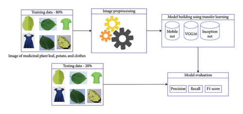
The main aspects of the study included data collection and annotation, image preprocessing, model building (feature extraction and training), and evaluation. Yet, a determined attempt was made to offer additional information about the study’s unique feature. Figure 2 shows the main activities that were flowed to achieve the study’s goal. It focuses primarily on the dataset preparation process, the model’s overall system design, preprocessing methods, creating machine-readable datasets, and model evaluation.
3.1. Datasets
Three types of datasets were employed, such as fashion, potato leaf images, and medicinal plant leaves. Building a model from scratch and gathering new datasets is not our primary goal. Rather evaluating the models’ performance for multilabel and multiclass classification with and without BN at the FC layer was the main objective of this work. We used the medicinal plant leaf dataset labeled (annotated) by 5 experts with 5, 10, 13, 28, and 30 years of experiences on herbal medicine [5]. Figure 3 and Tables 2 and 3 describe how we prepared the data. We collected the fashion and potato leaf dataset from Kaggle repository and prepared with the same method as medicinal plant.

| File name | Tags | Root | Bark | Leaf | Seed | Unidentified |
|---|---|---|---|---|---|---|
| Img_1 | [“Root”] | 1 | 0 | 0 | 0 | 0 |
| Img_2 | [“Root,” “leaf,” “seed”] | 1 | 0 | 1 | 1 | 0 |
| Img_3 | [“Bark,” “leaf”] | 0 | 1 | 1 | 0 | 0 |
| Img_4 | [“Seed”] | 0 | 0 | 0 | 1 | 0 |
| File name | Tags | Root | Bark | Leaf | Seed | Unidentified | Bark_leaf | Leaf_seed | Root_leaf |
|---|---|---|---|---|---|---|---|---|---|
| Img_1 | [“Root”] | 1 | 0 | 0 | 0 | 0 | 0 | 0 | 0 |
| Img_2 | [“Leaf_seed”] | 0 | 0 | 0 | 0 | 0 | 0 | 1 | 0 |
| Img_3 | [“Bark_leaf”] | 0 | 0 | 0 | 0 | 0 | 1 | 0 | 0 |
| Img_4 | [“Seed”] | 0 | 0 | 0 | 1 | 0 | 0 | 0 | 0 |
3.2. Image Preprocessing
The training platform’s computational capacity was taken into account while resizing the input image. For potato and fashion, we resize the image to 224 × 224. Despite the fact that Google Colab provided us 12 GB of RAM, the dataset contains a significant number of images of medicinal plants. So, to preserve computational resources, we reduced the input size to 64 × 64. Furthermore, we normalized image pixels across the board to decrease their range from 0 to 255 to 0 to 1. Learning gets slower when evaluating large-sized images with large integer values. As a result, the image’s pixels are normalized, or scaled down, to fall between 0 and 1. Ultimately, we stored a range of image pixel array values in a single variable for preservation. Lastly, to reduce processing time during the data loading process, we stored an array of image pixel values in a single variable with .npy format. We used RGB images even if the color feature requires computing time. RGB images reduce the loss of crucial leaf features.
We used the transfer learning technique to fine-tune the pretrained Mobile Net, VGG16, and Inception Net models. Using CNN, the feature extraction and training phases are completed concurrently. With the help of this CNN, the models were automatically trained to extract features from input images while it is learning. To obtain a unique identity from a given image and refine the pixel values, the CNN computes convolution operation by multiplying each image pixel by the kernel (weight) values. We used average pooling, ReLU, and the filtering kernel (convolution) to perform an automatic feature extraction technique.
3.3. Model Building
The standard convolutional neural network (S-CNN) and depthwise separable convolutional neural network (DWS-CNN)–based models are fine-tuned using transfer learning. VGG16 and Inception Net are selected from S-CNN while Mobile Net is from DWS-CNN. By using transfer learning, we could recognize and put into practice the information we have gained from previous tasks to new ones in a related domain. Being able to identify the domain’s commonalities is the crucial role of transfer learning [30, 31]. So, we achieved a good model performance with a small data, smaller epochs and short training times by adapting pretrained models. We tuned training and model hyperparameters using this transfer learning. We adjusted training parameters like learning rate, batch size, and optimizer. The FC network and CNN (learning layer) are two of the tuned model parameters. Figure 4 shows the customized architecture of Mobile Net.
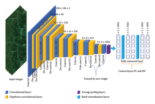
The last four CNN convolutional base (feature learning) layers of Mobile Net model are trained using the new weights, and the remaining layers are left frozen. It suggested that weights for frozen layers are not updated. ReLU activation functions and 1024-unit layers are utilized in four layers at the FC layer (classification layer).
All convolutional bases (feature learning layer) of Inception Net and VGG16 are frozen except the last two layers. For those two models, two dense layers and one BN layer are leveraged at the FC layer. Lastly, for multilabel and multiclass classification, we utilized the sigmoid and softmax activation layers, respectively. The addition of BN at the FC layer for both multilabel and multiclass classifier is an intriguing feature of this study. As a result, the models performed better and were trained quickly with fewer epochs.
3.3.1. The Difference Between S-CNN and DWS-CNN
S-CNN is applied in many pretrained models, which results in large parameter values because it completes the tasks of screening and integrating data features into a new set of output features all at once. Large training parameters require greater computational resources and take a long time to compute. The depthwise separable convolution in Mobile Net separates the convolution operation into two layers such as a filtering layer (depthwise convolution) and a combining layer (pointwise convolution). Every input channel receives a single filter deployment from the depthwise convolution. The outputs of the depthwise convolution are then combined with the pointwise convolution using a 1 × 1 convolution [32].
3.3.1.1. Standard Convolution
The following image sizes are not really used in this study. We took this size simply to illustrate how S-CNN and DWS-CNN operated to extract image features. Figure 5 shows an input image that is colored and sized by 12 × 12 × 3 pixels. Moreover, apply a 5 × 5 convolution with a stride of 1 and no padding to the image. The convolution technique is as follows. If we simply take the image’s width and height into account: 12 × 12 (5 × 5) = 8 × 8, every 25 pixels, the 5 × 5 kernel goes through to scalar multiplication, providing a single integer each time. An 8 × 8 pixel image is obtained because of the lack of padding (12 − 5 + 1 = 8). The colored image, however, has three channels. Therefore, three channels are required for the convolutional kernel. As a result, we compute 5 × 5 × 3 = 75 multiplications each time we convolve with an image pixel rather than 5 × 5 = 25. This image that is 12 × 12 × 3 becomes an 8 × 8 × 1 image after passing through a 5 × 5 × 3 kernel.
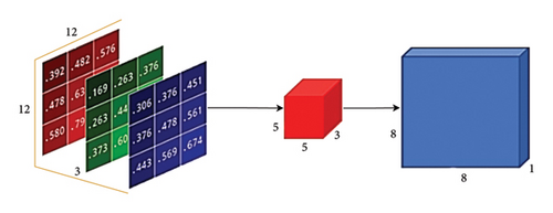
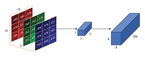
Let us use 256 filters for obtaining 256 8 × 8 × 1 image features, and building them together results in an output feature with a size of 8 × 8 × 256 as shown in Figure 6.

Thus far, we have observed the course of action of ordinary convolution. For more illustration, let us take filters with size of 5 × 5 × 3 × 256, where 5 × 5 × 3 × 256 stands for the filter’s height, width, number of input channels, and number of output features, respectively. When the input image with size of 12 × 12 × 3 convolved by 5 × 5 × 3 × 256 filters with stride =1 and padding=same, it produces ’= 12 × 12 × 256 feature maps.
3.3.1.2. Depthwise Separable Convolution
Nevertheless, a 12 × 12 × 3 image was transformed to 8 × 8 × 256 image features using the standard convolution method. However, the 12 × 12 × 3 image has been converted to 8 × 8 × 3 image features using depthwise convolution as indicated in Figure 7. We now have the opportunity to increase each image’s channel size. The reason that the pointwise convolution obtains its name is due to the fact it utilizes a 1 × 1 kernel or a kernel that iterates over every point. This kernel contains a depth of several channels (three in our example) in the input image. To build an 8 × 8 × 1 image, we operate a 1 × 1 × 3 kernel across our 8 × 8 × 3 image as shown in Figure 8.
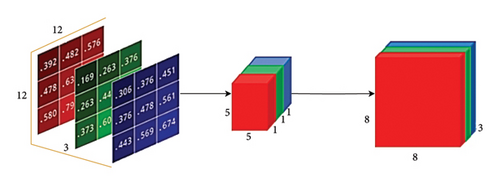
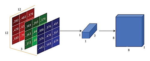
Every 5 × 5 × 1 kernel generates an 8 × 8 × 1 image by repeating through one channel of the image and obtaining the scalar products of each group of 25 pixels. An 8 × 8 × 3 image is made by layering these images together.
Figure 9 shows that we can create 256 1 × 1 × 3 kernels that create 8 × 8 × 1 images each to get a final image of shape 8 × 8 × 256.
Based on the above explanation, the model can compute the total parameters of 53,952 and 1,228,800 for standard and depthwise separable convolution, respectively. Hence, this huge difference makes the Mobile Net learn fast and perform accurate classification. That is the mystery of our intention emphasis for Mobile Net.
3.3.2. Model Evaluation
We instantly started the evaluation phase after training the model because it is necessary to validate the extent to which the model fulfills the requirements for classification. As a result, our evaluation measures include testing accuracy, precision, recall, and F1 score. The mathematical equations are given below, respectively.
3.3.3. How Does the Model Extract Image Features?
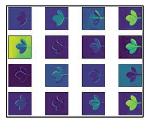
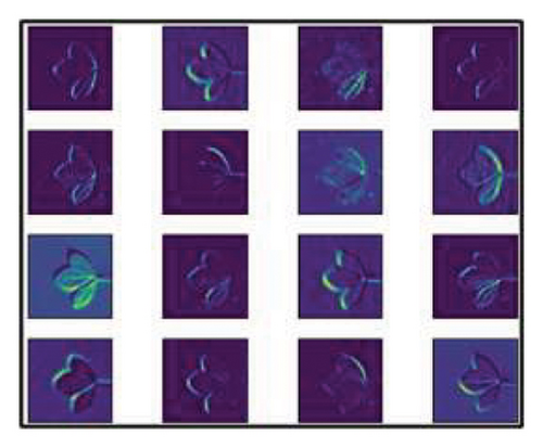
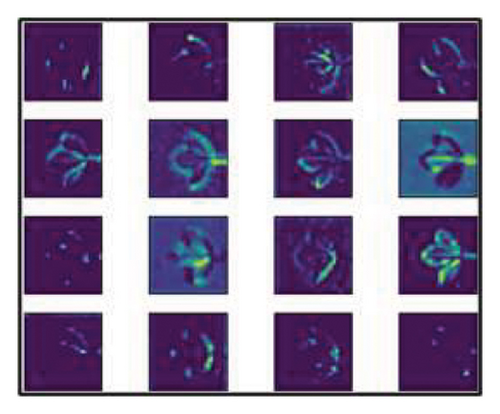
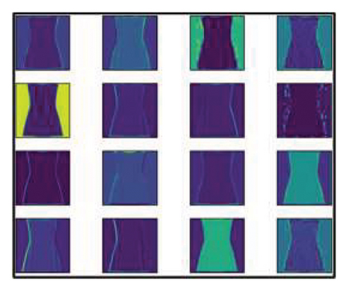
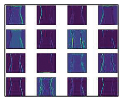
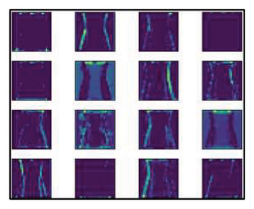
The process of extracting features from input data using CNN is illustrated in Figures 10 and 11. At the first convolution (the first layer), it recognizes just the horizontal and vertical lines that are present in the images. Because it can recognize various corners on input images, it attempts to figure out the shape of the item at the mid-level (2nd layer). CNN computed complex feature identification at the high level (3rd layer), which includes extracting variously arranged lines and shapes from an image’s surface. At the fourth and higher layer, CNN has a greater capacity to recognize very tiny image structures. Convolution could identify little portions of structure even as it goes into a very deep layer. CNN is able to detect patterns in images, determine their distinctive qualities, and build the data to be classified by the classifier layer. The number of features that the convolution layer computes is going to grow as the image size does.
3.3.4. Experimental Setup
3.3.4.1. Datasets
We trained and tested the models by three types of datasets such as fashion images, potato leaves, and leaves from medicinal plants. For both multilabel and multiclass classifiers, we employed the fashion and medicinal plant datasets. The potato dataset is exclusively utilized for multiclass classification. The quantity of training and testing data in each dataset is shown in Table 4. All datasets are split into 80% for the training set and 20% for the testing set.
| Datasets | Training data | Testing data | ||
|---|---|---|---|---|
| Input size | Total data | Input size | Total data | |
| Fashion image | 224, 224, 3 | 1944 | 224, 224, 3 | 486 |
| Medicinal plant leaf image | 64, 64, 3 | 12,080 | 64, 64, 3 | 3020 |
| Potato leaf image | 224, 224, 3 | 1200 | 224, 224, 3 | 300 |
3.3.4.2. Training and Testing Environment
For our experimental study, we used Google Collaboratory. Initially, we uploaded image data to Google Drive together with the relevant target labels (CSV files), and then we mounted the data on Google Collaboratory. We received a free workspace from Google Collaboratory equipped with a Tesla K80 GPRU0.0 and 12 GB of RAM for data preprocessing, building models (training), testing, evaluation, and prediction (classification).
3.3.4.3. Training Hyperparameters
In this study, we tried several experiments on multilabel and multiclass classification with and without BN at FC layers. We used testing accuracy and F1 score as model evaluation metrics. First, we tried different parameters using trial and error. Accordingly, we trained the models using a learning rate of 1 ∗10−3, 1 ∗10−4, and 1 ∗10−5; batch size of 32 and 64; and optimizers of Adamax and Adam. Finally, we selected a learning rate of 1 ∗10−4, Adam optimizer, and batch size of 32 for experimental analysis because we got better testing accuracies using these training parameters.
4. Results and Discussion
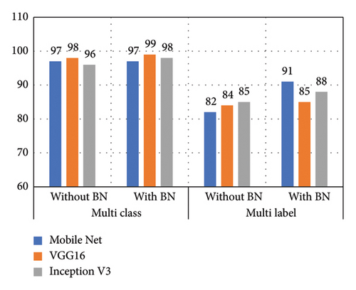
The main idea behind deep learning model building is how much it performs while tested by the new (unseen) data. Hence, in Tables 5 and 6, the study shows the testing accuracy of the model for multiclass and multilabel classification. The accuracy of the three models such as Mobile Net, VGG16, and Inception Net is evaluated for both multiclass and multilabel classification tasks, with and without BN at FC layers.
| Tuned models | Multiclass | Multilabel | ||
|---|---|---|---|---|
| Without BN | With BN | Without BN | With BN | |
| Mobile Net | 96.7 | 97 | 82.3 | 91 |
| VGG16 | 98.35 | 98.97 | 83.74 | 85.39 |
| Inception V3 | 96.3 | 97.53 | 85.39 | 87.65 |
| Tuned models | Multiclass | Multilabel | ||
|---|---|---|---|---|
| Without BN | With BN | Without BN | With BN | |
| Mobile Net | 99.2 | 99.2 | 83 | 93 |
| VGG16 | 98.51 | 99.07 | 77 | 84.3 |
| Inception V3 | 97.67 | 90.07 | 69 | 70.9 |
From Tables 5, 6, and 7, we can generalize that all models have better accuracy using multiclass classification than multilabel classification with all datasets because multilabel classification needs computing many mutually nonexclusive classes (labels) at the output layer. Training from a dataset that has mutually nonexclusive classes needs a lot of hidden layers and huge data by computing very complex parameters which leads the model confused with testing data.
| Tuned models | Multiclass | |
|---|---|---|
| Without BN | With BN | |
| Mobile Net | 97.8 | 99.3 |
| VGG16 | 97 | 97 |
| Inception V3 | 93.33 | 94 |
The above tables also showed that the testing accuracy of the model trained without BN at FC layers is lower than the model that has BN. This decrease of the performance occurred for both classification techniques because computing a large number of parameters at dense layers without BN created an internal covariant shift problem. Consequently, it makes the model decrease its accuracy. As indicated in Tables 5, 6, and 7, the models with BN achieved higher testing accuracy; especially for multilabel classifier, BN highly improved the performance of the model.
Multilabel classification computed multiple labels for a single input image that needs to capture complex relationship of medicinal plant leaf and fashion image features and labels. So, the model is more sensitive to the variation of the input distributions. We stabilized the training by normalizing the activations by leveraging BN at FC layers of each model and made the models to learn complex relationships easily. This makes the multilabel classifier attain a significant improvement in performance.
In multilabel classification, there are often correlations between labels; for example, fashion image has both “dress” and “blue” labels. Our BN at FC layers helped the model to capture these correlations by making the optimization landscape smoother and preventing internal covariate shifts. In contrast, the multiclass classifier model only needs capturing a simpler relationship like one correct class per input images. So, BN has no larger impact due to the more straightforward optimization process of the model.
Generally, in multilabel classifier, each label is predicted independently using a sigmoid activation function at the output layer. Especially when different labels have different scales, variability is created in the output distributions. We reduced this variability in the output distributions by normalizing the activations at FC layer using BN that makes the model converge faster and showed major performance improvement of multilabel classifier. On the other hand, multiclass classifier has a single output node where all categories are mutually exclusive that needs the operation of softmax activation function. So, there was smoother output distribution that reduced the potential benefit gained from BN.
4.1. Performance of a Model With Fashion and Medicinal Plant Datasets
Accuracy is not advisable for evaluating the model’s performance when the problem is multilabel classification and the dataset contains imbalanced data distribution. Accuracy does not take into account the model’s performance concerning individual classes. Therefore, we used F1 score to evaluate a model because F1 score is the most appropriate metric when there is imbalanced data distribution in each class; it is evident that all researchers used this metric for their model evaluation with imbalanced data, and this study followed suit.
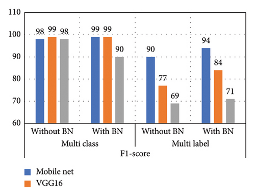
Figures 12 and 13 show the F1 score values of tuned Mobile Net, VGG16, and Inception Net models with and without BN at the FC layer of CNN for both multiclass and multilabel classifications. The performance of a model without BN at FC layer was reduced for multilabel classification than multiclass classification because in multilabel classification, the output space size grows exponentially with the number of possible labels, making it more difficult for the model to explore and predict all possible combinations accurately. In addition, there are no dependencies among different labels of our multilabel dataset. For example, in a medicinal plant dataset, the plant leaf is labeled with both “root,” “leaf,” and “seed.” In the fashion dataset, the cloth has both “jeans” and “black” and “jeans” and “blue” labels. Learning from these dependencies makes difficulties for a multilabel classifier model.
- i.
In multilabel classification, instances are associated with multiple classes simultaneously, making the problem more complex. Predicting multiple labels accurately for each instance requires more complex decision boundaries and can be inherently more challenging.
- ii.
Multilabel classification needs deeper CNN than multiclass classification. Figures 12 and 13 indicate deeper network tends to benefit more from BN. So, to get improved accuracy, BN at the dense layer of CNN is mandatory for multilabel classifier over multiclass.
4.2. Performance of a Model With Potato Leaf Dataset
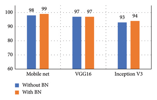
For this experiment, we evaluated only multiclass classification because the potato dataset has only three unique samples such as late blight, early blight, and healthy. It is not necessary to associate instances with multiple classes simultaneously.
As shown in Figures 11, 12, 13, and 14, there is no exaggerated improvement by leveraging BN at the dense layer of the multiclass classifier. In multiclass classification, each instance is assigned to exactly one class out of multiple mutually exclusive classes which makes the classification task simple because multiclass classification involves predicting only one label out of multiple possible labels for each instance at a time.
4.3. Mobile Applications and Predictions
The integration of a deep learning model with a mobile application holds a lot of potential for enhancing user experiences and providing innovative functions. Hence, we successfully integrated a model with the mobile application to test the models whether it can be applicable for real-world application or not. First, we changed the model into the TFLite model by which the model is ready for integration with mobile application. Secondly, we designed and developed the Android application by importing the TFLite model and corresponding target labels in Android studio. Figure 15 shows the procedure we followed to integrate the model with mobile app.
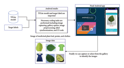
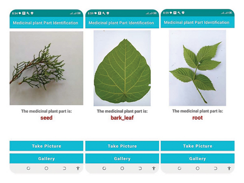
On the UI of the mobile app, there are three main components such as image display, result display capture button, and gallery button. Capture button is used to activate the mobile camera for capturing live photo, and gallery button is used to select the saved images from the gallery. The result component shows the corresponding identified labels of the captured or selected images.
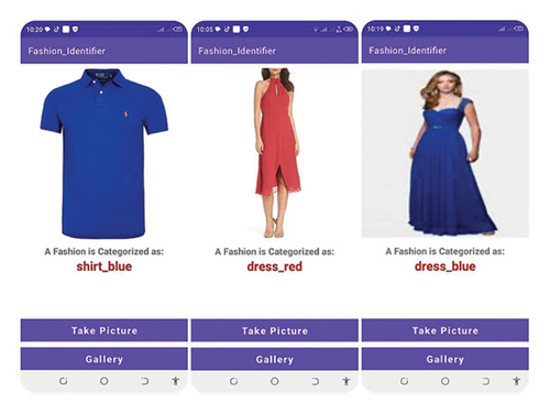
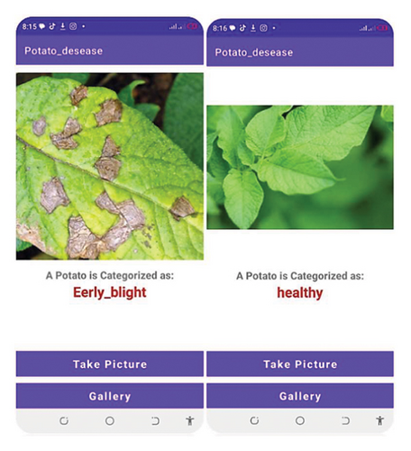
The result shown in Figure 16 may lead to a question of how the model predicts another part of the plant from leaf images? We used leaf images as identity of the remaining parts of the plant. Different plant parts are labeled (tagged) on the leaf image feature that is saved in the model. This implies that during supervised learning, image features are used only as an identity for the target label and labeling (mapping) is setting the target (true) values what we want from the classification result. That means we can tag (map) the target labels with identity image even though that labels are not part the training image. Figures 17 and 18 indicate the mobile application for fashion type and potato disease identification, respectively.
5. Conclusion and Future Work
5.1. Conclusion
This study’s primary goal was to determine how BN is important for a tuned model’s performance in multilabel and multiclass classification. Thereby, DWS-CNNs were used to train and build Mobile Net with and without BN layers at dense layers and compared with fine-tuned VGG16 and Inception Net models. Multilabel classification has numerous classifications in a single instance, in contrast to multiclass classification. Thus, multilabel classification is highly dependent on learning ambiguity and overfitting and requires more processing power, time, and hidden layers. The deep learning models were more confused by multilabel scenarios than multiclass. As a result, multilabel classifier model performance was worse than multiclass. Regarding that, the fine-tuned Mobile Net model achieved F1 scores of 97% and 91% for multiclass and multilabel classification using the fashion dataset. Using a dataset of medicinal plants, the model achieved 99% and 94% for multiclass and multilabel classification. This result proved that applying BN at the dense layer is an excellent strategy to develop a multilabel classifier model. Using three types of testing datasets, the study’s finding showed that BN leveraged at FC layers enhances the model performance for both multilabel and multiclass classifiers. According to the experimental results, BN significantly improves the model’s performance for multilabel classifier as compared to multiclass classifier.
5.2. Future Works
So far, we investigated the importance of leveraging BN at FC layer of CNN for both multilabel and multiclass classifier models by developing a fine-tuned model using three image datasets. We also tried to show how it looks like when integrated with the mobile application. But we integrated the model with mobile application only for test case. So, collecting huge data, training the model, and integrating the model with computer application will have realistic application. A model learned from huge image data needs a huge memory capacity that is beyond mobile devices’ capability. This study also uses three type datasets to test only three fine-tuned deep learning models using the transfer learning technique. Furthermore, fine-tuning many pretrained models and incorporating many datasets will enhance the robustness of the study findings toward the importance of BN for both multilabel and multiclass classifications.
Conflicts of Interest
The authors declare no conflicts of interest.
Author Contributions
Misganaw Aguate Widneh: data curation, data analysis and interpretation, visualization, methodology, document and code writing, reviewing, editing, and validation.
Amlakie Aschale Alemu: conceptualization, visualization, and original draft preparation and correction.
Dereje Derib Getie: conceptualization, visualization, and investigation.
Funding
The authors declare no funding for this research.
Acknowledgments
The authors have nothing to report.
Open Research
Data Availability Statement
The datasets generated and/or analyzed during the current study are not publicly available but are available from the corresponding author on reasonable request.


