Diabetes Prediction Using an Optimized Variational Quantum Classifier
Abstract
Quantum information processing introduces novel approaches for classical data encoding to encompass the complex patterns of input data of practical computational challenges using basic principles of quantum mechanics. The classification of diabetes is an example of a problem that can be efficiently resolved by using quantum unitary operations and the variational quantum classifier (VQC). This study demonstrates the effects of the number of qubits, types of feature maps, optimizers’ class, and the number of layers in the parametrized circuit, and the number of learnable parameters in ansatz influences the effectiveness of the VQC. In total, 76 variants of VQC are analyzed for four and eight qubits’ cases and their results are compared with six classical machine learning models to predict diabetes. Three different types of feature maps (Pauli, Z, and ZZ) are implemented during analysis in addition to three different optimizers (COBYLA, SPSA and SLSQP). Experiments are performed using the PIMA Indian Diabetes Dataset (PIDD). The results conclude that VQC with six layers embedded with an error correction scaling factor of 0.01 and having ZZ feature map and COBYLA optimizer outperforms other quantum variants. The optimal proposed model attained the accuracy of 0.85 and 0.80 for eight and four qubits’ cases, respectively. In addition, the final quantum model among 76 variants was compared with six classical machine learning models. The results suggest that the proposed VQC model has outperformed four classical models including SVM, random forest (RF), decision tree (DT), and linear regression (LR).
1. Introduction
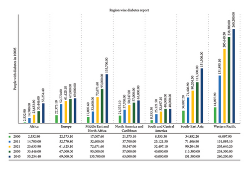
Diabetes is a major concern in global healthcare and has a profound impact on social and economic growth and public health worldwide. The global financial impact of diabetes was found to be $232 million in 2007 and increased to $966 billion in 2021 and estimated to be $1054 billion in 2045 [1]. Rapid growth and urbanization have led to an increase in this chronic disease that poses a severe danger to public health worldwide. In all age groups and environments, it is currently one of the most prevalent diseases. Between 1980 and 2014, the percentage of adults over 18 years of age who had diabetes increased dramatically from 4.7% to 8.5%, posing serious difficulties in industrialized and developing countries [2]. More than one and a half million people die annually as a result of it, making it the sixth most common cause of untimely death [3]. Currently, the International Diabetes Federation (IDF) [4] reports that there are 540 million people worldwide diagnosed as diabetic patients. According to IDF forecasts, the number of people living with diabetes is expected to increase by 46% to reach around 783 million, or 1 in 8 adults, by the year 2045. This huge number of expectations or future predictions could be reduced through different preventative measures and awareness campaigns. As illustrated in Figure 1, the most severely affected areas are in Southeast Asia and the southern Pacific, including China, India, and the United States of America. However, the spread of this surge is not uniform, as it is projected to reach 143% in Africa and 15% in Europe etc. This alarming percentage increase shall globally affect the adult population causing a reduction of lifetime and/or restricted life/food habits. The countries with higher populations shall have more economic impact to cure these deadly diseases, for example, China is the frontrunner with a population of 140.9 million, followed by India, Pakistan, USA, Indonesia, Brazil, Mexico, Bangladesh, Japan, Egypt etc. This deadly disease has drastic impacts on the functionality of vital body parts and unfortunately, there is no permanent solution currently except the diagnosis of this disease at an early stage or precise prediction so that patients can have preventive measures. Hence, there is a pressing demand for advanced technologies to diagnose diabetes early and automatically/noninvasively, ensuring greater precision.
Diabetes is an endocrine disease linked to the decreased capacity of the body to metabolize glucose, either due to insulin deficiency in general or to be produced by the pancreas. There exist four distinct forms of diabetes: Type 1 diabetes (T1D), also known as juvenile diabetes or insulin-dependent diabetes; Type 2 diabetes (T2D), also known as diabetes mellitus; the third one is gestational diabetes mellitus; and the fourth category is a type of diabetes that arise from other underlying factors [5]. Among these types, T1D and T2D are major and insulin-dependent diabetes. The first condition arises mainly due to the impaired functionality of pancreatic beta cells, whereas the second condition arises due to insufficient cellular absorption of insulin. Diabetic foot syndrome, heart attacks, strokes, liver cirrhosis, chronic renal failure, and other severe circumstances, sometimes fatal consequences, are associated with both T1D and T2D [6]. Deep learning (DL) and machine learning (ML) methods have been used in a variety of complicated problems to provide accurate and efficient results, since they have shown promising outcomes in discovering hidden patterns [7–9]. In recent years, numerous ML and DL frameworks have been proposed for the prediction of diabetes [10, 11] with different health conditions, including logistic regression, multilayer perceptron (MLP), random forest (RF), quadratic discriminant analysis (QDA), K-nearest neighbors (KNN), logistic regression, linear discriminant analysis (LDA), Naive Bayes (NB), artificial neural network (ANN), support vector machine (SVM), decision tree (DT), AdaBoost (AB), and radial basis function (RBF) [12]. The reported results showed that NB achieved the highest precision of 82% among ML algorithms including SVM, DT, and NV. Another study reveals that the Gaussian process (GP) classifier with ten-fold cross-validation outperforms LDA, QDA, and NB with 81.97% accuracy [13]. Furthermore, multiobjective optimization has been used to forecast diabetes using sequential minimum optimization, SVM, and elephant herding optimizer, with a precision rate of 78.21% [14].
The ML and DL models have provided what was expected, but there is still room for improvement in their precision before they can be widely used to predict diabetes. Recent advances in computing technology have enabled the processing of massive amounts of data. Quantum computing (QC) has demonstrated the ability to solve complicated problems much faster than traditional computing methodologies. Healthcare, in particular, will benefit from QC as the volume and diversity of health data increase dramatically [15]. QC techniques have proven to be more effective than conventional theory-based models in several domains, such as tracking, object identification, prediction, and classification. Inspired by this development, earlier research showed the utilization of QC to improve the performance of the classical ML and DL models [16]. The study [17] proposes quantum convolutional neural networks (QCNNs) for binary and multiclass classification of different quantum states, and reported results entail that hybrid QC algorithms have outperformed their classical equivalents. Similarly, an analysis of hybrid quantum-classical algorithms is provided in [18], with the goal of making quantum computer algorithms more efficient by suppressing errors using derivative-free optimization techniques. The authors in [19] proposed the techniques to extend the capabilities of the quantum variational eigen solver by introducing new methods to enhance its efficiency and lower the resource utilization to facilitate the practical implementation of quantum-based algorithms. The authors in [20] carry out a performance comparison of QML and DL techniques for diabetes prediction and explicate the merits and demerits of each approach. The presented work is highly informative in terms of comparing the efficiency of QML and DL used for medical diagnostics. The authors in [21] proposed an intelligent diagnostic system for T2D prediction utilizing the quantum particle swarm optimization (QPSO) algorithm incorporated with a weighted least squares SVM (WLS–SVM). The results show that combining QPSO with WLS–SVM is accurate in solving the problem of diabetes prediction. The authors in [22] discuss methods for classification problems, which are inspired by QC for the improvement of existing classification algorithms. This approach seems promising in enhancing the performance of classification tasks in many fields with specific emphasis on medical-related issues. The authors in [23] put forward the quantum-inspired neuroevolutionary algorithm for credit approval problems with both binary and real numbers representation. The proposed model shows better results in terms of managing more comprehensive credit approval tasks in comparison with conventional approaches. The authors in [24] proposed the model for feature extraction and classification from the EEG signals using quantum mechanics that demonstrate the improvements in using the quantum approaches for neurological signal processing. The requirement of a significant increase in EEG signal processing and classification is minimized with the help of the proposed framework. Overall, the proposed field of QC can deal with the diabetic data complications owing to certain factors including body structure, eating pattern, fat balance, and blood hemoglobin. Due to this capability, QC is effective for medical diagnostics especially for diabetes. Moreover, owing to the rapid development of technology, there emerges the essential need to shift from classical to quantum techniques for classification tasks in the medical domain to evaluate their efficiency and to assess their performance in comparison with classical techniques.
- 1.
Data preprocessing to remove noise, outliers, and replace missing values in PIDD by calculating the mean of attributes and then normalizing the data.
- 2.
PIDD density distribution and statistical analysis of all attributes with respect to class labels.
- 3.
Attribute (feature) selection through three different algorithms, namely, chi-square, extra tree classifier, and least absolute shrinkage and selection operator (LASSO). Depending on their highest score, four (glucose, insulin, BMI, and age) attributes are selected out of eight attributes.
- 4.
Design of the four-layered variational quantum classifier (VQC) for two sets of qubits, eight (with 40 parameters) and four (with 40 parameters) based on different number of attributes.
- 5.
Analysis of four-layered VQC with respect to three feature maps (Pauli, Z, and ZZ) and three optimizers (constrained optimization by linear approximation [COBYLA], simultaneous perturbation stochastic approximation [SPSA], and sequential least squares programming [SLSQP]) for both eight and four qubits, with a total of 18 variants.
- 6.
Analysis of designed VQC with respect to different number of layers, i.e., 2, 6, and 8 for both eight (with 24, 56, and 72 parameters) and four qubits (with 12, 28, and 36 parameters), with a total of 54 variants.
- 7.
Implementation of quantum error mitigation for VQC (QEMVQC) with different scaling factors (λ = 1, 0.1, 0.2, and 0.01), with a total of 4 variants.
- 8.
Implementation of six CML (LR, DT, RF, GB, XGBOOST, and SVM) using eight and four attributes of PIDD, with a total of 12 variants.
- 9.
In general, 76 variants of QML-based VQC were designed in this study compared with 12 CML variants.
- 10.
Detailed performance comparison analysis of QML and CML models for PIDD based on different evaluation matrices and future directions.
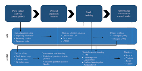
The following is the outline of the remaining sections of the paper. The materials and methods utilized in this study are described in Section 2 including overall methodology, compute resources used for experiments, the details of dataset |and preprocessing, VQC for diabetes prediction, QEMVQC, and evaluation matrices used in the research. Section 3 provides a detailed analysis and comparison of results based on different scenarios with discussion. Section 4 provides a conclusion of the current study.
2. Materials and Methods
This section is subdivided into six subsections (A ∼ F), which include the following: compute resources for experiments, dataset details with its preprocessing, quantum classifier (VQC) used for diabetes prediction, error mitigation technique for VQC, and different evaluation matrices used to assess the performance of all models. These are discussed in detail in this section.
2.1. Compute Resources
All QML and CML models used in this study are implemented on the GPU system (RTX 3090) and IBM_Brisbane with 127 qubits that also support open Qasm3 based upon Python programming environment and a variety of Python Keras and Qiskit libraries. Table 1 presents the hardware and simulator specifications used for the experimental setup and their specifications.
| S# | Name | Specifications |
|---|---|---|
| 1 | Python | 3.11.4 |
| 2 | OS | Windows 11 |
| 3 | CPU | 11 intel(R) core (TM) i9-9700F CPU @ 3.00 GHz |
| 4 | RAM | 16 GB |
| 5 | GPU | RTX 3090 with 48 GB RAM |
| Simulation setup | ||
| 1 | Qiskit | 0.44.2 |
| 2 | Qiskit-terra | 0.25.2 |
| 3 | Qiskit_Aer | 0.12.2 |
| 4 | Qiskit_machine_learning | 0.6.1 |
| 5 | IBM_Brisbane | Processor type: Eagle r3 |
2.2. Dataset
The data are considered as oil for AI, and it plays a core role in the training of any AI model through classical and/or quantum techniques. In addition, the preprocessing steps to extract useful information/features and to remove outliers/noise from data also improve the outcome/performance of the trained model. The updated version of PIDD, which can be downloaded from the UCI Machine Learning Repository: https://archive.ics.uci.edu/ml/support/Diabetes (accessed on 21 December 2023), is used in this study. The data were acquired from 768 female subjects in the age group of 21–25 years. Among these subjects, 268 subjects were diagnosed with diabetes before experimentation and the remaining 500 individuals were in better health, i.e., nondiabetic. Eight essential attributes along with labels listed as outcomes were acquired during the data acquisition process and those parameters are listed in Table 2 with their respective description. Figure 3 also displays the density distribution of all attributes of the PIDD dataset with respect to labels.
| S# | Attributes | Attributes’ description |
|---|---|---|
| 1 | Age | Age in years |
| 2 | Diabetes pedigree function | Diabetes pedigree function |
| 3 | BMI | Body mass index (weight in kg/height in cm) |
| 4 | Insulin | 2-Hour serum insulin (U/mL) |
| 5 | Skin thickness | Skin fold thickness (mm) |
| 6 | Blood pressure | Diastolic blood pressure (mm·Hg) |
| 7 | Glucose | Plasma glucose concentration |
| 8 | Pregnancies | Number of times pregnant |
| 9 | Outcome | Outcome (0 and 1) |

2.3. Data Preprocessing and Attribute Selection
Data preprocessing handles duplicate and unbalanced data, which are highly correlated with low-variance variables in the dataset, missing values, and outliers. Consequently, the preprocessing techniques used in this study include the removal of outliers, filling missing values with a mean of that attribute, and data normalization. Table 3 provides the statistical analysis of the PIDD including mean, standard deviation, and maximum and minimum values of all attributes after preprocessing.
| S# | Attributes | Mean | Standard deviation | Minimum | Maximum |
|---|---|---|---|---|---|
| 1 | Pregnancies | 3.84 | 3.36 | 0 | 17 |
| 2 | Glucose | 121.6 | 30.46 | 44 | 199 |
| 3 | Blood pressure | 74.8 | 16.68 | 24 | 142 |
| 4 | Skin thickness | 56.89 | 44.51 | 7 | 142 |
| 5 | Insulin | 139.42 | 87.24 | 14 | 846 |
| 6 | BMI | 33.63 | 12.22 | 18 | 142 |
| 7 | Diabetes pedigree | 0.47 | 0.33 | 0 | 2.42 |
| 8 | Age | 33.24 | 11.76 | 21 | 81 |
| 9 | Outcome | 0.34 | 0.47 | 0 | 1 |
Optimal feature selection from data is performed through three different algorithms. Table 4 provides the summary of attribute selection algorithms, namely, the chi-square test, extra trees, and LASSO. The score calculated against each attribute is mentioned in Table 4 as well. Each method provides a unique perspective on attribute importance: the chi-square test deals with the relationships between categorical variables, extra trees combines the results coming from DTs, and LASSO employs regularization to make the selection of features even more accurate. We selected the attributes with the highest score, e.g., using the chi-square test, the most valuable attributes for the classification are “insulin” (6779.24) and “glucose” (1537.20), while “age” (189.30) and “BMI” (108.32) are also important. Extra trees indicated that “glucose” is the most important attribute with the highest score of 0.230 followed by “insulin” with the score of 0.147, while “BMI” comes third with 0.123, and lastly “age” with 0.128. LASSO indicates “glucose” as the most relevant having a value of 0.0065 ,followed by” insulin” 0.0004, while “BMI” attains a score of 0.0006 and “age,” a score of 0.0002.
| S# | Attributes | Chi-square test | Extra trees | LASSO |
|---|---|---|---|---|
| 1 | No. of pregnancies | 110.54 | 0.105 | 0.00 |
| 2 | Glucose | 1537.20 | 0.230 | 0.0065 |
| 3 | Blood pressure | 54.26 | 0.089 | 0.0 |
| 4 | Skin thickness | 145.20 | 0.090 | 0.0 |
| 5 | Insulin | 6779.24 | 0.147 | 0.0004 |
| 6 | BMI | 108.32 | 0.123 | 0.0006 |
| 7 | Age | 189.30 | 0.128 | 0.0002 |
| 8 | Diabetes pedigree | 4.30 | 0.128 | 0.0 |
- Note: Bold values signify the highest scores.
Data preprocessing of PIDD and attribute selection reduce the dimensionality and the complexity of VQC and CML models. This step results in utilizing computational resources optimally and reduces inference time as well. Therefore, the removal of noise and appropriate attribute selection techniques are very important for increasing performance, understandability, and the sparing of computational resources in predictive modeling.
2.4. VQC for Diabetes Prediction
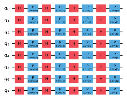
The classification problem in AI refers to the association of a sample of input data to one of the output classes. Let us consider , i = 1, 2, 3, M to be the input feature vector corresponding to one of the output classes Yi = [y1, …, yk]. The resultant of the trained AI model is a mapping that transforms the input vector Xi to the predicted value/class . The difference between predicted class and actual class yi is the loss or error of prediction. Similarly, in QML, the classification problem is initialized by converting the classical feature vector Xi to a quantum counterpart |Xi〉 through data encoding schemes. There are several encoding schemes such as basis encoding, amplitude encoding, and angle encoding.
VQC is a hybrid quantum-classical optimization framework that consists of a shallow quantum classifier and is interconnected with the classical optimizer part. The architecture of VQC is depicted in Figure 4(a). It has several compartments such as cost function, ansatz, gradient approach, and optimizers. Three major components of VQC are depicted from equations (1)–(7), namely, data encoding, followed by parametrized quantum circuit, and the final component is the measurement part. The encoding part is necessary for classical data, while in the case of quantum data, this component can be omitted.

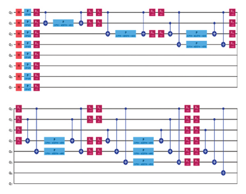
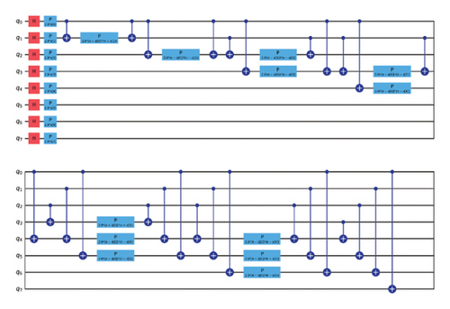
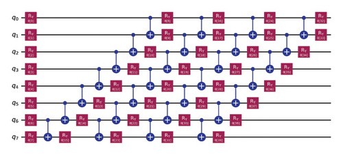
For each input Xi, is predicted by VQC, that is, the probability of measurement.
2.5. QEMVQC for VQC
VQC are considered as effective QML models for the near future in the era of noisy intermediate–scale quantum (NISQ). These algorithms have shown several useful applications in real-life scenarios such as classification and pattern recognition in complex data. Recently many different versions of VQC including parametric quantum classifiers (PQCs) have been proposed, but they all share a common foundation of parametric or ansatz based on tunable parameters [27]. The values of these parameters are adjusted throughout the training process utilizing the optimization process.
However, due to quantum hardware and simulator’s limitations, a large number of optimization algorithms result in a complex situation. This change will shift the minimal or optimal values of the loss function and therefore, restrict the applicability of NISQ devices for such algorithms. Besides, VQC models are threatened with a problem called noise-induced barren plateaus (NIBPs) where noise results in vanishing gradients, thus hindering optimization [28].
To avoid these problems, we need to create a fault-tolerant architecture with a desired number of logical qubits or to minimize noise in the results of NISQ hardware. Therefore, attaining noise-free quantum hardware is time taking, but currently, QEM techniques [29] can play their role to eliminate noise up to a certain level. It is also important to mention that QEM may not eliminate exponential loss concentration, and rather it will help to enhance trainability by minimizing loss contamination. Thus, the authors in [30] introduce an algorithm to perform real-time quantum error mitigation (RTQEM) in VQC training.
For each iteration, the scaled QEMVQC is added to the gradient of the cost function in order to make the convergence of VQC smooth and help it to find global minima by avoiding the local minima.
2.6. Evaluation Matrices
TN is true negative: Patients with diabetes predicted as normal/healthy by models.
FP is false positive: Patients without diabetes or healthy patients are predicted as diabetic by models.
FN is false negative: Patients with diabetes predicted as normal/healthy by models.
3. Results and Discussion
- •
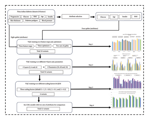
Step 1: Analysis of four-layered VQC with respect to two sets of qubits: four qubits (with 20 parameters) and eight qubits (with 40 parameters) and three feature maps (Pauli, Z, and ZZ) and three optimizers (COBYLA, SPSA, and SLSQP). A total of eighteen (2 × 3 × 3 = 18) variants are presented in Subsection A.
- •
Step 2: This step involves further enhancement and analysis of 18 variants designed in Step 1. The changes include variations in a number of layers and corresponding parameters. This step is further divided into two parts:
- (i)
2-a: For eight qubits, the case number of layers is 2, 6, and 8 (as 4-layered was considered in Step 1) with 24, 56, and 72 parameters, respectively.
- (ii)
2-b: For four qubits, the case number of layers is 2, 6, and 8 (as 4-layered was considered in Step 1) with 12, 28, and 36 parameters.
- (i)
- •
Therefore, total 54 (18 × 3 = 54) variants were analyzed in this step. The results of the best 24 among 54 variants are presented in Subsection B.
- •
Step 3: The best-performing variant, based upon analysis in Step 2 is selected for Step 3 to have QEMVQC analysis using four different scaling factors λ = 1, 0.1, 0.2, and 0.01. Thus, this step designs four new (1 × 4 = 4) variants based on the optimal model of Step 2. The results related to four variants designed in this step are presented in Subsection C
- •
Step 4: Lastly, six CML models, namely, LR, SVM, DT, RF, XGBOOST, and GB, using four and eight attributes are implemented for performance comparisons. Therefore, a total of 12 (6 × 2 = 12) variants of CML are analyzed for comparison with our proposed best VQC variant (6-layered with QEM and λ = 0.01) among 76 VQC variants.
3.1. Results Analysis of VQC With Respect to Qubits, Feature Maps, and Optimizers
This subsection provides the results of the current study through VQC using different qubits (attributes) and by employing three distinct (Pauli, Z, and ZZ) feature maps and three (COBYLA, SPSA, and SLSQP) optimizers. Table 5 provides the detailed comparison analysis of accuracies and Type 1 and Type 2 errors for all 18 variants of VQC on test data.
| VQC variant | Feature map | Optimizer | Accuracy | Type 1 error | Type 2 error |
|---|---|---|---|---|---|
| Four qubits | Pauli feature map | COBYLA | 0.59 | 0.41 | 0.42 |
| SPSA | 0.56 | 0.44 | 0.45 | ||
| SLSQP | 0.52 | 0.48 | 0.48 | ||
| Z feature map | COBYLA | 0.69 | 0.29 | 0.32 | |
| SPSA | 0.62 | 0.36 | 0.39 | ||
| SLSQP | 0.58 | 0.41 | 0.42 | ||
| ZZ feature map | COBYLA | 0.76 | 0.21 | 0.26 | |
| SPSA | 0.69 | 0.3 | 0.33 | ||
| SLSQP | 0.73 | 0.24 | 0.29 | ||
| Eight qubits | Pauli feature map | COBYLA | 0.66 | 0.33 | 0.35 |
| SPSA | 0.62 | 0.37 | 0.39 | ||
| SLSQP | 0.57 | 0.42 | 0.44 | ||
| Z feature map | COBYLA | 0.74 | 0.23 | 0.28 | |
| SPSA | 0.73 | 0.24 | 0.29 | ||
| SLSQP | 0.7 | 0.27 | 0.31 | ||
| ZZ feature map | COBYLA | 0.81 | 0.18 | 0.19 | |
| SPSA | 0.78 | 0.21 | 0.23 | ||
| SLSQP | 0.75 | 0.24 | 0.26 | ||
- Note: Bold values signify the highest scores.
It has been observed that VQC with Pauli feature map and COBYLA optimizer achieved an accuracy of 0.59 and 0.66, thereby minimizing Type 1 and Type 2 errors from 0.41 and 0.42 to 0.33 and 0.35 corresponding to four qubits and eight qubits, respectively. In contrast, the SPSA optimizer performed less effectively compared to the COBYLA optimizer with accuracies of 0.56 and 0.62 and improved Type 1 and Type 2 errors from 0.44 and 0.45 to 0.37 and 0.39 corresponding to four and eight qubits, respectively. SLSQP optimizer is least accurate with 0.52 and 0.57 accuracies for four and eight qubits, thereby depicting Type 1 and 2 errors’ reduction from 0.48 and 0.49 to 0.42 and 0.44, respectively.
Similarly, the Z feature map with COBYLA optimizer obtained the accuracy of 0.69 and 0.74 with improved Type 1 and Type 2 errors from 0.29 and 0.32 to 0.23 and 0.28 corresponding to four and eight qubits, respectively. SPSA optimizer performed quite well, having accuracy from 0.62 to 0.73 respectively for four and eight qubit cases with Type 1 and Type 2 errors from 0.36 and 0.39 to 0.24 and 0.29 obtained by using four and eight qubits, respectively. The SLSQP optimizer reported accuracy of 0.58 and 0.70 with improved Type 1 and Type 2 errors from 0.41 and 0.42 to 0.27 and 0.31 using four and eight qubits, respectively.
In the case of the ZZ feature map, the COBYLA optimizer provided the highest accuracy of 0.76 and 0.81 for four and eight qubits while improving Type 1 and Type 2 errors from 0.21 and 0.26 to 0.18 and 0.19, respectively. The SPSA optimizer also exhibited good performance with accuracies of 0.69 and 0.78 for four and eight qubits with improved Type 1 and Type 2 errors from 0.30 and 0.33 to 0.21 and 0.23. Lastly, the SLSQP optimizer obtained accuracies of 0.73 and 0.75, using four and eight qubits with improved Type 1 and Type 2 errors from 0.24 and 0.29 to 0.24 and 0.26 respectively.
All these results emphasize the importance of feature map selection and the optimization methods to improve the performance of VQC in this case.
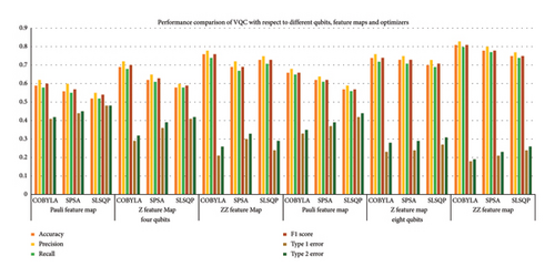
Figure 6 provides a comparison of all 18 variants of VQC across various optimization strategies and all evaluation matrices. It is evident that VQC with the ZZ feature map and COBYLA optimizer achieved the best results among others for both four and eight qubits. It achieves the highest accuracy value of 0.81, precision value of 0.83, recall value of 0.8, Type 1 error of 0.18, and Type 2 error of 0.19, using all eight attributes. Similarly, with four attributes, it exhibits better results as compared to Z and Pauli feature maps. The Z feature map also showed good performance with COBYLA with an accuracy of 0.74. On the contrary, the Pauli feature map generally exhibits low performance particularly with SLSQP for both four and eight qubits cases. These results assert the effectiveness of the ZZ feature map and the COBYLA optimizer in improving VQC’s efficacy.
3.2. Results Analysis of VQC With Respect to Different Numbers of Layers and Parameters (θs)
This subsection provides the analysis of variants designed with variations in the number of layers in addition to the previous variations. All variants designed in Step 1 are further analyzed with a variation of layers (2, 6, and 8). Hence, a total of 54 variants were designed. The six best variants of Step 1 correspond to a total of 24 variants whose results are presented in this section. The overall results corresponding to the 24 best cases of this step are shown in Figure 7. The variants designed in this case indicated that parametric circuits having six layers performed better than others, followed by four-layered cases. The number of parameters in the case of six-layered cases was 28 and 56 corresponding to four- and eight-qubit circuits, respectively. The performance of six-layered VQC was better in terms of accuracy, precision, recall, F1 score, and Type 1 and Type 2 errors as compared to the rest of the three cases, i.e., VQC with 2-, 4-, and 8-layered parametric circuits. It is important to mention that the four-layered case performed very close to the six-layered case.
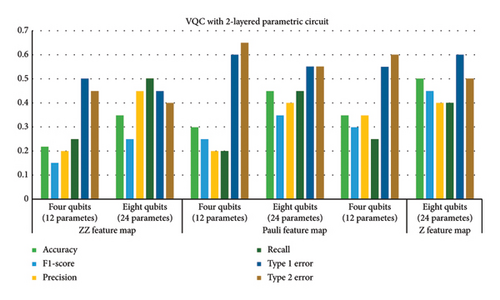
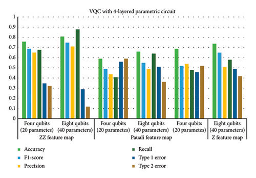
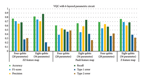
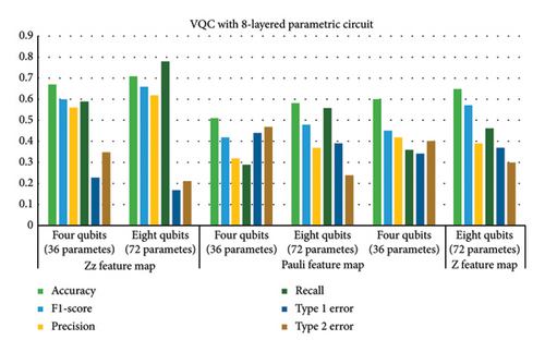
Therefore, Table 6 provides the detailed analysis of these two best VQC cases corresponding to three feature maps with COBYLA optimizer. Table 6 contains two subsections involving four- and six-layered cases’ results respectively. Comparing the results from both the sections of Table 6 reveals notable differences in the performance of various feature maps and qubit configurations. It is evident from tabular data in Table 6 that increasing the number of qubits generally enhances the performance of VQC, but the extent of improvement depends on the feature map class. Four-layered VQC results show that in the case of the ZZ feature map, accuracy increases from 0.76 to 0.81 by increasing qubits from four to eight, respectively. For six-layered VQC with ZZ feature maps, accuracy increases from 0.77 to 0.82 by increasing qubits from four to eight, respectively. Similarly, in these two cases, F1 score for the ZZ feature map rises from 0.69 to 0.75 and from 0.71 to 0.75, respectively. This indicates a consistent improvement in performance with more qubits for the ZZ feature map across both evaluations.
| 4-layered VQC with # parameters = 20 and 40 for four and eight qubits | 6-layered VQC with # parameters = 28 and 56 for four and eight qubits | |||||||||||
|---|---|---|---|---|---|---|---|---|---|---|---|---|
| Evaluation metrics | ZZ feature map | Pauli feature map | Z feature map | ZZ feature map | Pauli feature map | Z feature map | ||||||
| Four qubits | Eight qubits | Four qubits | Eight qubits | Four qubits | Eight qubits | Four qubits | Eight qubits | Four qubits | Eight qubits | Four qubits | Eight qubits | |
| Accuracy | 0.76 | 0.81 | 0.59 | 0.66 | 0.69 | 0.74 | 0.77 | 0.82 | 0.61 | 0.66 | 0.69 | 0.76 |
| F1 score | 0.69 | 0.75 | 0.49 | 0.55 | 0.52 | 0.65 | 0.71 | 0.75 | 0.39 | 0.45 | 0.54 | 0.69 |
| Precision | 0.65 | 0.71 | 0.44 | 0.49 | 0.54 | 0.51 | 0.65 | 0.71 | 0.54 | 0.59 | 0.64 | 0.61 |
| Recall | 0.68 | 0.88 | 0.41 | 0.64 | 0.48 | 0.58 | 0.68 | 0.88 | 0.51 | 0.74 | 0.58 | 0.68 |
| Type 1 error | 0.35 | 0.29 | 0.56 | 0.51 | 0.46 | 0.49 | 0.28 | 0.21 | 0.46 | 0.41 | 0.36 | 0.39 |
| Type 2 error | 0.32 | 0.12 | 0.59 | 0.36 | 0.52 | 0.42 | 0.31 | 0.11 | 0.49 | 0.26 | 0.42 | 0.32 |
In contrast, the Pauli feature map demonstrates less consistent results. Accuracy improves from 0.59 to 0.66 and from 0.61 to 0.66 across the sections of tables corresponding to four- and six-layered VQC, but this increase is less pronounced compared to the ZZ feature map. The F1 score for he Pauli feature map also shows modest improvement from 0.49 to 0.55 and from 0.39 to 0.45, which suggests that the benefit of adding qubits is less significant for the Pauli feature map.
The Z feature map exhibits mixed results as well. Accuracy improves from 0.69 to 0.74 and from 0.69 to 0.76, while the F1 score increases from 0.52 to 0.65 and from 0.54 to 0.69. This indicates a general trend of improvement with more qubits, though not as pronounced as with the ZZ feature map.
Type 1 and Type 2 errors decrease with the increase in qubits for all feature maps. For instance, the Type 1 error for the ZZ feature map drops from 0.35 to 0.29 and from 0.28 to 0.21, demonstrating enhanced performance with more qubits. Type 2 errors also decrease consistently across feature maps, reinforcing the trend of improved performance with additional qubits. Overall, the ZZ feature map consistently outperforms others, particularly with eight qubits, while the Pauli and Z feature maps show less improvement.
3.3. Performance Evaluation of VQC Variant With Six-Layered Parametric Circuit With Respect to QEMVQC and Scaling Factor (λ)
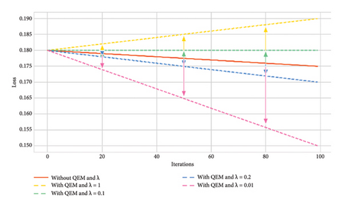
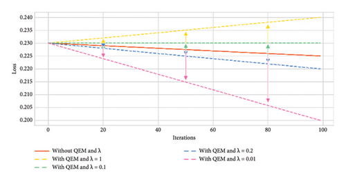
The resultant variant of VQC in Step 2 was a six-layered VQC with a ZZ feature map having the COBYLA optimizer. This subsection summarizes the results of effects on an optimal variant of Step 2 through the error mitigation technique for VQC having different values of scaling factor (λ) under four and eight qubit cases. The value of scaling factors is considered to be 1, 0.1, 0.2, and 0.01. Thus, four new variants corresponding to each four and eight qubits were analyzed on the optimal VQC model of Step 2. Table 7 presents the results of these eight versions of VQC for all evaluation matrices. Similarly, Figure 8 presents the accuracy and loss plots of these four VQC variants for both eight and four qubits.
| Evaluation metric | 6-layered VQC without QEM and scaling factor (λ) | 6-layered VQC with QEM and scaling factor (λ = 1) | 6-layered VQC with QEM and scaling factor (λ = 0.2) | 6-layered VQC with QEM and scaling factor (λ = 0.1) | 6-layered VQC with QEM and scaling factor (λ = 0.01) | |||||
|---|---|---|---|---|---|---|---|---|---|---|
| Four qubits | Eight qubits | Four qubits | Eight qubits | Four qubits | Eight qubits | Four qubits | Eight qubits | Four qubits | Eight qubits | |
| Accuracy | 0.77 | 0.82 | 0.76 | 0.81 | 0.78 | 0.83 | 0.77 | 0.82 | 0.80 | 0.85 |
| F1 core | 0.71 | 0.75 | 0.69 | 0.75 | 0.71 | 0.77 | 0.7 | 0.76 | 0.73 | 0.79 |
| Precision | 0.65 | 0.71 | 0.65 | 0.71 | 0.68 | 0.73 | 0.67 | 0.72 | 0.7 | 0.76 |
| Recall | 0.68 | 0.88 | 0.68 | 0.88 | 0.7 | 0.9 | 0.69 | 0.89 | 0.72 | 0.91 |
| Type I error | 0.28 | 0.21 | 0.35 | 0.29 | 0.33 | 0.27 | 0.34 | 0.28 | 0.3 | 0.24 |
| Type II error | 0.31 | 0.11 | 0.32 | 0.12 | 0.3 | 0.1 | 0.31 | 0.11 | 0.27 | 0.08 |
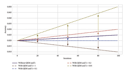
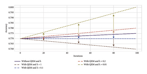
The proposed VQC model accuracy tends to improve by reducing the scaling factor λ from 1 to 0.01. Notably, the highest accuracy of 0.85 is achieved for eight qubits with λ = 0.01. In contrast, without QEM, the accuracy is lower, i.e., 0.77 and 0.82 for four and eight qubit models, respectively.
The F1 score reflects the balance between precision and recall. It ranges from 0.69 to 0.79, using eight qubits and λ = 0.01. It again indicates the improved performance of this variant of VQC as compared to λ = 1, 0.2, and 0.1.
Precision values are consistent, but the highest precision of 0.76 is reached for eight qubits with λ = 0.01, demonstrating that the model’s prediction for positive outcomes improves as λ decreases.
The recall is highest at 0.91 with eight qubits and λ = 0.01, showing the model’s ability to capture most true positives effectively. Without QEM, recall is notably lower at 0.68 for both four and eight qubits.
Type I errors (false positives) decrease with the use of QEM, especially for smaller scaling factors. The smallest Type I error of 0.21 occurs with eight qubits without QEMVQC. Similarly, Type II errors (false negatives) show improvement as λ decreases, with the lowest value of 0.08 for eight qubits.
These improved results suggest that QEMVQC with smaller scaling factors helps to mitigate issues such as barren plateaus and local minima and improves the convergence of quantum models. Similarly, lower error rates indicate that QEMVQC helped the proposed VQC model avoid local minimal to navigate the optimization landscape more effectively, thus improving the overall performance and robustness of the proposed model. This also suggests that the model is less likely to get stuck in suboptimal solutions and can generalize better with the reduced scaling factor and QEM, particularly for eight qubits.
3.4. Performance Comparison of Six CML Models Having Six-Layered VQC Variant With QEMVQC and λ = 0.01
This subsection summarizes the results of six CML models, LR, DT, GB, XGBOOST, RF, and SVM, and their comparison with the optimal variant of VQC selected from Step 3 (six-layered VQC with QEMVQC and λ = 0.01 using four and eight attributes). Table 8 and Figure 9 present these results and their comparisons based upon all evaluation matrices.
| Evaluation metrics | LR | DT | GB | XGBOOST | RF | SVM | Ours (6-layered VQC [with QEM and λ = 0.01]) | |||||||
|---|---|---|---|---|---|---|---|---|---|---|---|---|---|---|
| Four qubits | Eigh qubits | Four qubits | Eight qubits | Four qubits | Eight qubits | Four qubits | Eight qubits | Four qubits | Eight qubits | Four qubits | Eight qubits | Four qubits | Eight qubits | |
| Accuracy | 0.68 | 0.73 | 0.63 | 0.72 | 0.88 | 0.96 | 0.86 | 0.95 | 0.65 | 0.79 | 0.76 | 0.81 | 0.8 | 0.85 |
| F1 score | 0.69 | 0.75 | 0.65 | 0.71 | 0.81 | 0.93 | 0.88 | 0.91 | 0.66 | 0.78 | 0.76 | 0.82 | 0.73 | 0.79 |
| Precision | 0.67 | 0.74 | 0.63 | 0.72 | 0.85 | 0.98 | 0.87 | 0.88 | 0.65 | 0.78 | 0.7 | 0.81 | 0.7 | 0.76 |
| Recall | 0.65 | 0.78 | 0.68 | 0.7 | 0.77 | 0.86 | 0.89 | 0.95 | 0.6 | 0.8 | 0.74 | 0.84 | 0.72 | 0.91 |
| Type 1 error | 0.33 | 0.26 | 0.37 | 0.28 | 0.15 | 0.02 | 0.13 | 0.05 | 0.35 | 0.22 | 0.3 | 0.19 | 0.3 | 0.24 |
| Type 2 error | 0.35 | 0.22 | 0.32 | 0.3 | 0.23 | 0.14 | 0.11 | 0.05 | 0.4 | 0.2 | 0.26 | 0.16 | 0.27 | 0.08 |
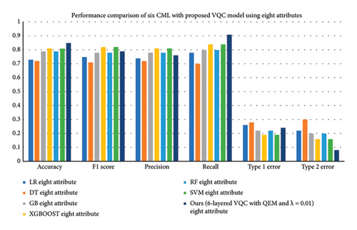
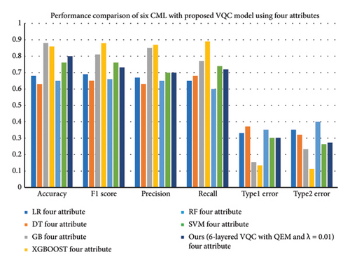
This work demonstrates how the use of CML models to predict diabetes is based on whether eight or four attributes are used. The CML models, which incorporate all eight of the features, can utilize a wider range of input variables as they cover all eight attributes of PIDD. Therefore, they can analyze simple and complex patterns and relationships in data. With the help of the increased dimensionality or attributes, it is possible to identify an interaction between several factors that influence diabetes with a higher degree of accuracy. It is noteworthy that in the case of a four-attribute input space, these CML models can work in a rather restricted spectrum. This could lead to a certain amount of information loss, but it provides an avenue for increased computational and interpretational advantages. In both situations, there seems to be a ‘trade-off’ between interpretability and dimensionality. The eight-attribute model offers enhanced functionality and performance. Conversely, the four-attribute architecture provides a prediction model that is not only less complicated but also potentially easier to understand, but their performance lacks the classifiers with original data as input. In addition, four-feature models are less complex compared to the other variants in terms of execution time and resource utilization. It is evident that XGBoost and GB outperform other CML models based on the selected attributes, including LR, DT, RF, and SVM, as well, for accurately predicting diabetes.
The results presented in Table 8 highlight the performance comparison of various CML and a six-layered VQC with QEM and a scaling factor (λ = 0.01) across different evaluation metrics, using both four and eight attributes. Notably, GB, XGBoost, and our proposed VQC model consistently outperform LR, DT, RF, and SVM in terms of accuracy, precision, recall, and F1 score, particularly when using eight attributes.
The maximum accuracy is with GB (0.96) and XGBoost (0.95) using eight attributes, while the proposed VQC model results in an accuracy of 0.85. Also, the results for the four attributes indicate that the VQC model has a better generalization compared to SVM and RF with an accuracy of 0.80 and this shows higher performance than compared to traditional models such as LR and DT. Furthermore, our VQC with QEM consistently demonstrates lower Type 1 and Type 2 error rates compared to classical models, with Type 1 errors reducing to 0.24 for the eight-attribute case and Type 2 errors dropping to 0.08, which is competitive with XGBoost.
Precision and recall are some of the most important assessment parameters to judge the performance of classification especially when dealing with unbalanced datasets The VQC model achieved a precision of 0.76 and recall of 0.91 in the eight-attribute case in comparison with GB and XGBoost with higher precision. When it comes to recall, the proposed VQC with QEM demonstrates better performance, which indicates a potential increase in sensitivity to true positives.
Overall, for the F1 score, our VQC model shows good performance, achieving a score of 0.79 for eight attributes. Based on the F1 score, VQC seems to be more effective in achieving a good balance between precision and recall for both sets of attributes, and thus, it is effective in classification scenarios. In general, the addition of QEMVQC improves the overall classification accuracy, but more importantly, decreases error rates to make it a potential replacement for CML models, especially for the datasets with less features.
This comprehensive result analysis of all VQC variants has yielded insightful findings on their performance across various configurations, including different qubit counts, feature maps, optimizers, different number of layers, QEMVQC, and comparison with CML models. It is analyzed that decreasing the number of qubits from eight to four is the best choice for optimal use of computed resources, and it also reduces the model complexity. However, as far as VQC performance is concerned, it is observed that VQC, with eight numbers of qubits, constantly outperforms the variants with four qubits in all cases. This improved performance, no doubt, underscores the potential of VQCs to handle more patterns and correlations of attributes for classification tasks as the quantum system scales up by using a large number of qubits. The impact of using different feature maps, i.e., Pauli, Z, and ZZ feature maps: It is observed that throughout the experiments, the ZZ feature map consistently outperforms both the Pauli and Z feature maps in terms of accuracy, F1 score, and Type 1 and Type 2 errors. All these results emphasize the importance of ZZ feature maps in improving the performance of all VQC variants. The impact of using different optimizers, i.e., COBYLA, SPSA, and SLSQP: It is observed that COBYLA optimizers tend to perform better than SPSA and SLSQP across various configurations of qubits and feature maps, particularly with the ZZ feature map. For instance, in the four-qubit setup with the ZZ feature map, COBYLA achieved an accuracy of 0.76, whereas SPSA and SLSQP yielded lower accuracies. Similarly, using eight qubits, and with the ZZ feature map, it achieved an accuracy of 0.81, which is much higher than SPSA and SLSQP optimizers. This analysis suggests that the COBYLA optimizer offers better convergence of VQC.
The effectiveness of QEMVQC with varying scaling factors (λ) showed a notable improvement in the performance of VQC. For example, in six-layered VQC with different configurations of qubits and with a scaling factor of λ = 0.01 led to higher accuracy and F1 scores compared to configurations without QEMVQC or with other scaling factors. This indicates that QEMVQC can significantly enhance the robustness of VQC, although its effectiveness may vary with different λ values.
4. Conclusions
This study thoroughly investigates the suitability of VQC for predicting diabetes by highlighting the critical insights into their performance across different configurations of qubits, feature maps, optimizers, number of layers and parameters, and finally through QEMVQC. As the number of qubits increases to eight, a superior performance of VQC is consistently observed as compared to four-qubit configurations. There is a notable improvement in the performance of VQC when ZZ feature maps with COBYLA optimizer are used as compared to Pauli and Z feature maps. Similarly, accuracy, F1 score, precision, recall, and Type 1 and 2 errors improved as the number of layers in VQC increased to six from four layers with an increased number of learnable parameters. In addition, QEMVQC with a suitable scaling factor particularly with λ = 0.01 significantly enhanced the accuracy of VQC to 0.85 and showed promising results for diabetes prediction when compared to CML models. However, from all these achievements, we still observe that there is a scope for improvement in VQC to outperform CML models.
Thus, the findings of this study reveal that QML has the capacity to achieve better results than CML methods in future by using more qubits and parameters, especially if physical quantum computers are available. They will surpass CML algorithms in precision as well as speed. Furthermore, it would be beneficial to carry out more experiments with a large number of parameters to enhance the efficiency of VQC for complex problems. In future, we aim to conduct additional experiments with various parameters to optimize the efficiency of VQC for complex datasets.
Conflicts of Interest
The authors declare no conflicts of interest.
Funding
This work was supported by the Artificial Intelligence Technology Centre, NCP (Quantum Machine Learning and Cognitive Computing Laboratory, Islamabad (4400), Pakistan). This work was supported by a National Research Foundation (NRF) Grant Funded by the Korean government (MSIT) (2022R1C1C2003637) (to K.S.K). This work was supported by the Global Joint Research Program funded by the Pukyong National University (202411510001) (to K.S.K).
Acknowledgments
This work was supported by the Artificial Intelligence Technology Centre, NCP (Quantum Machine Learning and Cognitive Computing Laboratory, Islamabad (4400), Pakistan). This work was supported by a National Research Foundation (NRF) grant funded by the Korean government (MSIT) (2022R1C1C2003637) (to K.S.K). This work was supported by the Global Joint Research Program funded by the Pukyong National University (202411510001) (to K.S.K).
Open Research
Data Availability Statement
The dataset used in this study will be available on request.


