CO2- and PM2.5-Focused Optimal Ventilation Strategy Based on Predictive Control
Abstract
This study developed and evaluated an optimal ventilation strategy for variable air volume (VAV) systems, targeting carbon dioxide (CO2) and particulate matter less than 2.5 μm in diameter (PM2.5) concentrations. The strategy integrates system-level demand-controlled ventilation (DCV) based on real-time occupancy data and zone-level predictive control using indoor air quality (IAQ) prediction models. By predicting indoor CO2 and PM2.5 levels for the subsequent time step and dynamically adjusting control priorities, optimal airflow is determined. A co-simulation model integrating EnergyPlus, CONTAM, and Python was employed for model training and testing. The proposed strategy was compared with on–off control, CO2 predictive control, and PM2.5 predictive control, demonstrating superior prediction accuracy and stable IAQ maintenance. The optimal ventilation strategy achieved the highest performance, maintaining CO2 and PM2.5 levels below their respective upper limits of 100% and 97.33% of the time. Although this strategy resulted in slightly higher energy consumption compared to the other control algorithms due to its multivariable control approach, it effectively maintained IAQ standards. This method simplifies development and maintenance by circumventing the need for complex optimization, providing a flexible and cost-effective solution for IAQ management. Future research will focus on developing integrated VAV system control strategies that ensure comfort year-round, addressing both energy efficiency and thermal comfort.
1. Introduction
The significance of indoor air quality (IAQ) has been increasingly emphasized since individuals spend an average of 90% of their time indoors [1]. Effective ventilation is crucial for maintaining IAQ, which directly impacts the health and productivity of occupants. Fresh outdoor air can be introduced through either natural or mechanical ventilation. While natural ventilation can be easily achieved by opening windows in residential settings, mechanical ventilation is predominantly used in commercial buildings, office facilities, and hospitals where central HVAC systems are installed.
Mechanical ventilation systems commonly regulate outdoor air intake based on indicators such as carbon dioxide (CO2) concentration or outdoor air temperature. However, IAQ cannot be adequately assessed using a single pollutant. The World Health Organization (WHO) defines key pollutants for air quality assessment, including particulate matter (particulate matter less than 10 μm in diameter (PM10) and particulate matter less than 2.5 μm in diameter (PM2.5)), ozone, nitrogen dioxide, sulfur dioxide, and carbon monoxide [2]. Among these, PM2.5, with aerodynamic diameters less than 2.5 μm, is particularly detrimental to human health [3, 4]. PM2.5 originates from both outdoor sources, such as traffic and construction, and indoor sources, such as occupant activities. While filters can be installed in ventilation systems to prevent the ingress of outdoor PM2.5, high-efficiency particulate air (HEPA) filters are rarely used in central HVAC systems due to their resistance to airflow, which can increase energy consumption. Consequently, portable air purifiers are increasingly utilized to reduce indoor PM2.5 levels.
In workplaces, where individuals spend a significant portion of their time, ventilation and temperature control are managed through variable air volume (VAV) systems. During heating or cooling periods, VAV terminal units adjust the supply airflow rate based on the indoor air temperature or to ensure the minimum airflow rate [5–7]. Conversely, during nonconditioning periods when temperature control is not required, VAV systems are either not operated or operated intermittently based on monitored indoor CO2 levels. However, relying on a single variable for ventilation can negatively impact IAQ. For instance, indoor CO2 concentration is primarily dependent on the rate of outdoor air intake. In contrast, introducing outdoor air when outdoor PM2.5 levels are higher than indoor levels can exacerbate indoor PM2.5 concentrations. Therefore, in situations where temperature control is not necessary, a ventilation strategy that comprehensively considers both CO2 and PM2.5 is essential to maintain healthy IAQ for occupants.
To achieve simultaneous control of CO2 and PM2.5 in VAV systems, solutions that manage multiple environmental variables using limited resources, such as outdoor air intake rates and indoor supply airflow adjustments, are required. These solutions are predominantly investigated under the concept of optimal control, with prominent methods including model predictive control (MPC) and artificial intelligence (AI)–based control. MPC derives optimal control scenarios by predicting the system’s dynamic behavior and environmental conditions based on system manipulations. This prediction-based control method helps maintain indoor environmental comfort by minimizing the duration that target environmental variables exceed acceptable levels [8–10]. Multiobjective optimization algorithms can define objective functions for various control variables and simultaneously optimize these functions to identify the best control parameters. For example, Anand et al. [11] integrated MPC with rule-based control to optimize the air handling unit (AHU) model and zone temperature through mathematical modeling and real-time occupancy data, achieving minimal outdoor air intake while controlling the supply air of the VAV terminal. Ganesh et al. [12] developed a physics-based building model to control dedicated ventilation systems using MPC, considering the dynamics of ozone, formaldehyde, particulate matter, and energy. This approach optimized IAQ while minimizing energy consumption through iterative optimization at each timestep. Li et al. [13] focused on minimizing system energy use and disease transmission risk, using Pareto optimization to derive a set of optimal solutions, further refined by membership functions to extract the best solution.
Over recent decades, AI has gained significant traction in building indoor environment control, particularly as an alternative to address the limitations of MPC. Traditionally, MPC utilized mathematical models to predict and regulate indoor environments, whereas AI-based optimal control leverages data-driven models, offering a streamlined approach to model creation based on measured data without the need to mathematically define complex input–output relationships. By tailoring machine learning algorithms to the specific characteristics of the data, data-driven models can significantly enhance prediction performance. Furthermore, AI-based models can adapt to new environments through training of real-time data or historical data on daily, weekly, or monthly bases. Adapting to new environments, whether through supervised or unsupervised methods, requires substantial data for accuracy [14]. However, this challenge has been increasingly addressed through research demonstrating the feasibility of real-time model learning [15–17].
Leveraging these advancements, studies on AI-based multiobjective control have been actively pursued. For instance, Hou et al. [18] developed predicted mean vote (PMV) and CO2 prediction models using an extreme learning machine (ELM) optimized with the grey wolf optimizer (GWO) algorithm. Their models predicted PMV and CO2 under various system control scenarios and calculated energy consumption to identify the control variables with the highest performance score based on a scoring function. Similarly, Cho et al. [13] employed neural network-based models to predict PMV, CO2, PM10, and PM2.5. They defined objective functions for each predicted value, merged them into a single objective function using a weighted sum approach, and determined optimal temperature setpoints and ventilation airflow rates. Kim et al. [19] utilized artificial neural networks (ANNs) to create prediction models for indoor load, CO2 concentration, and energy consumption, using these predictions to optimize airflow rate and supply air temperature under minimal energy conditions.
As noted in previous studies, technologies that can be utilized to simultaneously control CO2 and PM2.5 levels are being researched continuously. However, comprehensive consideration of IAQ across various factors is not present in many studies, and robustness across different environments is also often overlooked. From the perspective of building applicability, higher performance may be achieved by control algorithms developed specifically for certain buildings or systems; however, disadvantages in terms of applicability, maintenance, and cost-effectiveness may arise. For example, expert involvement is necessitated by MPC to define system models and objective functions. Additionally, numerous parameters are required to improve the accuracy of the system model, making calibration essential [20]. As a result of these factors, the general applicability of MPC across different systems is limited by its nature [21].
Many AI-based optimal control methods do not function autonomously. In most instances, a machine learning model serves as a predictor for buildings or systems, while optimization functions determine the control values. Yadav et al. [22] developed a recurrent neural network model to predict hour-ahead cooling loads, employing a weighted sum–based optimization function to minimize operational costs. Similarly, Reynolds [23] created an ANN-based model that predicts indoor air temperature and building energy consumption, utilizing a genetic algorithm (GA) to optimize energy consumption while maintaining thermal comfort. Afram et al. [24] developed multiple ANN models representing subsystems of HVAC systems, which were integrated into a MPC framework. An optimization function was employed to minimize the costs associated with the HVAC system. In defining the optimization functions, cost functions that combine various target values into a single expression are necessary. However, these cost functions are dependent on the applied system, which can diminish the applicability of control algorithms. Therefore, to enhance applicability and robustness across variable environments, the development of flexible ventilation control strategies is essential which can effectively substitute the functionality of optimization functions without relying on them.
- •
An optimal indoor air pollutant control method applicable during unconditioned periods, emphasizing IAQ
- •
A multivariable control strategy that operates robustly across various environments without heavy reliance on optimization functions, distinguishing it from conventional optimization-based controls
- •
A novel co-simulation approach linking EnergyPlus, CONTAM, and Python to demonstrate intelligent IAQ control feasibility, overcoming previous limitations in this area
The results of this study provide not only a contaminant-focused control method for VAV systems but also introduce promising avenues for future researchers aiming to develop more efficient IAQ control strategies. Furthermore, these findings suggest practical applications for energy-efficient, adaptive ventilation in modern buildings, with potential to improve occupant health and reduce operational costs.
2. Methodology
2.1. Research Overview
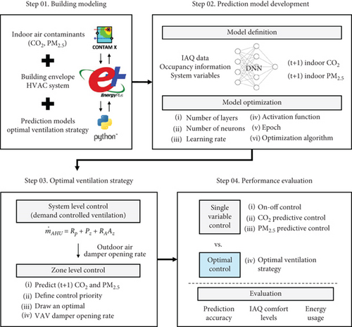
The research process, as depicted in Figure 1, comprises four distinct stages. The first stage involves building modeling. A comprehensive analysis of the thermal environment, IAQ, and energy consumption was conducted using a co-simulation technique that integrates EnergyPlus, CONTAM, and Python. The developed building model served as a basis for data acquisition and performance evaluation. In the second stage, prediction models for indoor CO2 and PM2.5 were developed. Input data were selected based on the mass balance equation, and a DNN model was constructed. The final prediction models were determined through a training process that included hyperparameter optimization. The third stage focused on the development of the optimal ventilation strategy. The established prediction models were integrated, and an algorithm for determining the control priority between the two environmental variables was configured to iterate at each time step. The final stage entailed performance evaluation. To validate the performance of the optimal ventilation strategy, CO2-based on–off control and single-variable control methods based on DNN, specifically CO2 predictive control and PM2.5 predictive control, were defined. Simulations were conducted for each scenario to analyze the prediction accuracy of the prediction models, the IAQ comfort level under different control strategies, the energy usage, and the control performance under varying filter conditions.
2.2. Building Model
Research on indoor air pollutants requires meticulous attention to safety during experiments due to the potential health risks to occupants. Consequently, many studies utilize computer simulations to conduct related research [25–27]. To model indoor air pollutants and their dynamics, information such as infiltration, generation rate, resuspension rate, removal rate, and deposition rate is required. However, obtaining these data through field measurements is often challenging or impossible, leading many studies to use assumed values in mathematical models or rely on statistical models. Therefore, this study employed the small office prototype building model provided by the US Department of Energy (DOE). This model represents approximately 70% of the floor areas of commercial buildings in the United States [28] and is used for building indoor environments and energy simulations in various studies as well as revisions of ASHRAE (American Society of Heating, Refrigerating, and Air-Conditioning Engineers) Standards [29–31]. The prototype building model is provided for both EnergyPlus and CONTAM, ensuring consistency in boundary conditions between different simulation tools, which enhances stability. Detailed information about the building can be found in Reference [32]. The building consists of south, north, east, west, and core zones and is a single-story structure. The HVAC system is set to a default constant air volume (CAV) system, with approximately 30 occupants.
For effective performance evaluation of the optimal ventilation strategy, few information in the existing building model was modified. First, the HVAC system was changed to a VAV system because the fixed indoor supply airflow rate in the CAV system does not allow for the optimal airflow calculation resulting from the control strategy. The AHU serves the entire building, while each zone has one VAV terminal, totaling five. Second, the occupancy schedule was adjusted for each zone on weekdays to introduce environmental variation, as occupants are sources of CO2 and PM2.5. A uniform occupancy schedule across zones would not provide diverse control results. Lastly, the PM2.5 filtration efficiency was set to 80%. While HEPA filters can capture over 99% of PM2.5, this level of filtration would eliminate nearly all PM2.5 impacts from outdoor air intake and cause a decrease in supply airflow rate due to increased static pressure.
Since this model does not simulate an actual building, validation through calibration was challenging to apply. Therefore, to ensure the validity of input specification changes, the building energy consumption was compared against the original model to confirm that no abnormal discrepancies were found. For evaluation, the coefficient of variance of the root mean squared error (CVRMSE) metric suggested by ASHRAE Guideline 14 was used [33]. It was observed that the CVRMSE for monthly and hourly energy consumption was 8% and 15%, respectively, meeting the allowable limits of 15% and 30%. These results indicate that HVAC adjustments and change of input specifications were conducted within a normal range.
2.3. Co-simulation Framework
To evaluate the performance of machine learning–based ventilation control, a building simulation tool capable of real-time calculations for thermal environment, air quality, energy, and control algorithms is necessary. However, a tool that provides all these functions simultaneously does not yet exist [34]. Therefore, this study constructed a co-simulation architecture using EnergyPlus, CONTAM, and Python. EnergyPlus provides the building envelope, HVAC system, and energy model. CONTAM models indoor air pollutants and calculates concentrations by considering temperature, differential pressure, infiltration, and ventilation. Python enables the application of machine learning–based prediction models and customized control algorithms. Since Version 9.3, EnergyPlus has offered a Python API, allowing Python to replace energy management system (EMS). This enables the use of libraries for data processing or machine learning, facilitating the implementation of prediction models and the optimal ventilation strategy.
The interconnection of each tool is shown in Figure 2, where data generated from the simulation results are exchanged at each timestep. EnergyPlus and CONTAM communicate via the functional mock-up interface (FMI) standard. Weather data, indoor thermal environments, occupancy, and HVAC system operation data are transmitted from EnergyPlus to CONTAM. Based on this information, CONTAM calculates infiltration, indoor CO2, and PM2.5 concentrations and sends these values back to EnergyPlus. These values are transmitted to EMS and output variables, which Python can then retrieve. The optimal ventilation strategy is designed to predict indoor CO2 and PM2.5 concentrations and determine the optimal operation of the ventilation system based on the current state at each timestep. To achieve this, Python retrieves weather, indoor thermal environments, indoor CO2 and PM2.5, occupancy, and HVAC system operation data from EnergyPlus and sends back the predicted CO2 and PM2.5 values along with the optimal AHU and VAV terminal damper positions. EnergyPlus then uses these values to control the ventilation system and calculate energy consumption.
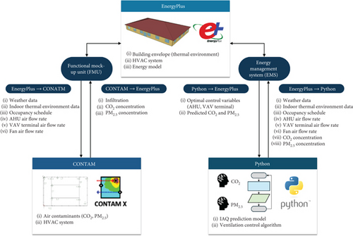
In this co-simulation process, data delay between the tools is inevitable. For instance, even if the AHU outdoor air damper position is derived from Python, it is not immediately reflected in the system within EnergyPlus and subsequently communicated to CONTAM within a single timestep. This delay can affect the immediacy of indoor environment control, but this can be mitigated by minimizing the simulation timestep [35]. EnergyPlus allows a minimum timestep of 1 min. Therefore, the simulation was conducted with this timestep, and it was observed that environmental changes due to damper positions input from Python were reflected after four timesteps. Consequently, ventilation system control and data interpretation were conducted at 5-min intervals.
2.4. IAQ Prediction Models
In this study, IAQ prediction models refer to the indoor CO2 prediction model and the indoor PM2.5 prediction model. Each model predicts the one-step-ahead concentration of CO2 and PM2.5, serving as critical components of the optimal ventilation strategy. As data-driven models, these IAQ prediction models are developed using field-acquired data and follow a supervised learning approach. Common machine learning algorithms used for indoor environmental prediction include support vector machines, k-nearest neighbors, decision trees, random forests, and neural networks. Among these, neural networks are particularly advantageous for learning nonlinear relationships between input and output data and have relatively low computational costs [36]. Additionally, neural networks are not overly complex to develop and can be incrementally trained, making them widely used for indoor environment prediction, building energy consumption forecasting, MPC, and intelligent control applications [37–39].
Neural networks are further categorized based on the connection methods of nodes and learning techniques. Among these, DNNs feature multiple hidden layers, providing superior performance with fewer nodes compared to single-layer neural networks [40]. The target variables for control in this study, indoor CO2 and PM2.5, are influenced by multiple factors such as infiltration, outdoor concentration, indoor sources, and removal rates, exhibiting nonlinear relationships that do not remain constant even under the same conditions. Moreover, most of these independent variables are challenging to measure in real time using sensors. Considering the characteristics of CO2 and PM2.5, DNNs were employed to develop the IAQ prediction models. The training process is summarized in Figure 3.
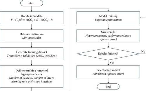
Among the variables in this equation, data directly obtainable via sensors include the concentration of outdoor and indoor air pollutants and the VAV terminal opening rate representing the supply airflow rate. Additionally, the AHU damper opening rate was included as it influences the concentration of mixed indoor pollutants. For the generation rate, occupant count data were used indirectly, as occupants are the primary sources of CO2 and PM2.5 through respiration and activity. The removal rate, comprising disposal rate and mass, was excluded from the input data due to the lack of real-time sensor data acquisition. The selected input data was subjected to a data normalization process using the min–max scaler from the scikit-learn library, scaling each data point between 0 and 1. This process prevents overfitting and increased dependency on specific independent variables due to differing data scales, thereby improving learning efficiency. The normalized data were then divided into training (60%), validation (20%), and test data (20%) sets for the training process.
The performance of prediction models is influenced by the number of hidden layers, the number of neurons in each layer, and variables such as the optimization function, epochs, batch size, and learning rate. These variables are defined as hyperparameters, and the optimal combination must be identified to achieve the best performance of the prediction models. This study applied Bayesian optimization (BO) to iteratively determine the optimal hyperparameters through repeated training. BO selects the optimal hyperparameters through the interaction between a surrogate model and an acquisition function [41]. The surrogate model probabilistically estimates the unknown shape of the objective function based on the combination of forecasting model results and hyperparameters. The acquisition function recommends hyperparameter combinations, iteratively seeking the combination that maximizes the performance of the objective function. The number of search iterations was set to 20. After each search, the combination of hyperparameters and the validation result defined by mean squared error (MSE) were recorded. Upon completing the predetermined number of searches, the model with the lowest MSE among the 20 candidates was selected as the final model. The structure of the IAQ prediction models is depicted in Figure 4.

2.5. Optimal Ventilation Strategy
- •
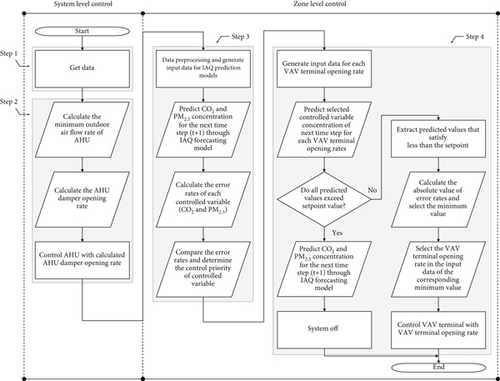
Step 1: Acquire the current time step data required for CO2 and PM2.5 prediction and optimal control. The data includes outdoor CO2 concentration, outdoor PM2.5 concentration, indoor CO2 concentration, indoor PM2.5 concentration, outdoor air damper opening rate, VAV terminal opening rate, and the number of occupants.
- •
Step 2: Input the occupancy data into the equation for calculating the minimum outdoor air intake, as shown in Equation (2). This equation represents the DCV-CO2 control method presented in ASHRAE Standard 62.1 [43]. DCV-CO2 enables stable calculation of the minimum outdoor air intake by responding in real time to the changing number of occupants, in addition to the required ventilation per building area. For efficient utilization of this equation, real-time occupancy data acquisition is necessary. Recent advancements in sensor and deep learning technologies have introduced methods such as infrared (IR) or deep vision–based people counters [44, 45] and Wi-Fi connection–based occupancy inference [46] which provides high counting accuracy. For single-zone systems, the total number of occupants is used, while for multizone systems, the zone with the highest occupancy is considered.
- •
Step 3: Generate input data for the IAQ prediction models. Here, the AHU damper opening rate uses the value calculated in Step 2, and the remaining data are from the current time step acquired in Step 1. This data is then input into the IAQ prediction models to forecast CO2 and PM2.5 concentrations for the next time step. The errors between the predicted values and the upper limits for each control variable are calculated using Equations (4) and (5), with the larger error selected as the control priority.
- •
Step 4: Implement control based on the selected control priority. In this step, predictions are made for all possible VAV terminal opening rates. Unlike the prediction in Step 3, which forecasts how indoor CO2 or PM2.5 will change if the current state is maintained, this step is aimed at determining the minimum airflow rate required to keep CO2 or PM2.5 below their upper limits. Therefore, instead of using the current VAV terminal opening rate, six different opening rates (ranging from 0 to 1 in increments of 0.2) are used to generate input data. Instead of using the current VAV terminal opening rate, six different opening rates (ranging from 0 to 1 in increments of 0.2) are used to generate input data. For each of these six opening rates, the IAQ prediction models forecast the indoor CO2 or PM2.5 levels. These predicted values are then compared to their respective upper limits. If all predicted values exceed the upper limits, the VAV terminal is fully opened to ensure maximum ventilation. However, if at least one predicted value does not exceed the upper limit, the VAV terminal opening rate that results in the smallest absolute error between the predicted value and the upper limit is selected. This approach ensures that IAQ remains within comfortable and safe limits by preventing CO2 and PM2.5 levels from exceeding their upper limits while optimizing the use of ventilation resources.
2.6. Evaluation Metrics
3. Result Analysis
3.1. Training Results of IAQ Prediction Models
Simulations were conducted to generate training data for the control scenarios of the AHU and VAV systems. The control variables included the AHU damper opening rate and the VAV terminal opening rate, each incremented from 0 to 1 in steps of 0.2. To introduce variability in CO2 and PM2.5 levels beyond the fixed schedules of arrival, lunch, and departure times, the number of occupants during other times was adjusted arbitrarily. Weather data and outdoor CO2 and PM2.5 concentration data were sourced from previous studies, specifically selecting a week with significant PM2.5 fluctuations based on actual sensor data [48]. This simulation yielded a total of 72,576 data points, which were then normalized and separated to form the training dataset.
The hyperparameters optimized via BO included the number of hidden layers, the number of neurons per layer, the learning rate, and the activation function. The detailed search ranges for these hyperparameters are provided in Table 1. Given the absence of predefined criteria for hyperparameter selection, the search ranges were arbitrarily set to balance training efficiency. The optimization algorithm employed was Adam optimization, with the number of epochs set to 100 and a batch size of 32. The BO process involved 20 iterative learning trials. The CO2 and PM2.5 prediction models were trained independently.
| Hyperparameters | Bayesian optimization | Range and value |
|---|---|---|
| Number of hidden layers | ✓ | 1–5 |
| Number of neurons of each layer | ✓ | 10–30, step: 2 |
| Learning rate | ✓ | 0.01, 0.001, 0.0001 |
| Activation function | ✓ | Sigmoid, Tanh, ReLu |
| Epochs | — | 100 |
| Optimization algorithm | — | Adam optimization |
| Trials | — | 20 |
The results of the training are summarized in Table 2 and Figure 6. For the CO2 prediction model, BO identified an optimal architecture with 2 hidden layers containing 8 and 12 neurons, respectively. The learning rate was set at 0.001, and the ReLU (rectified linear unit) activation function was used. The training outcomes demonstrated high prediction accuracy, with a MAE of 3.50 ppm, a CVRMSE of 0.85%, and an R2 value of 0.99. Similarly, the PM2.5 prediction model exhibited excellent performance, featuring an architecture with 3 hidden layers containing 10, 10, and 6 neurons, respectively. The learning rate was 0.001, and the ReLU activation function was employed. The PM2.5 prediction model achieved a MAE of 0.12 μg/m3, a CVRMSE of 1.50%, and an R2 value of 0.99. Figure 6 presents scatter plots of the actual versus predicted values for both models, with no outliers detected.
| Model | Optimization results | Metrics | ||||
|---|---|---|---|---|---|---|
| Structure | Learning rate | Activation function | MAE | CVRMSE | R2 | |
| CO2 prediction model | 5-8-12-1 | 0.001 | ReLu | 3.50 ppm | 0.85% | 0.99 |
| PM2.5 prediction model | 5-10-10-6-1 | 0.001 | ReLu | 0.12 μg/m3 | 1.50% | 0.99 |
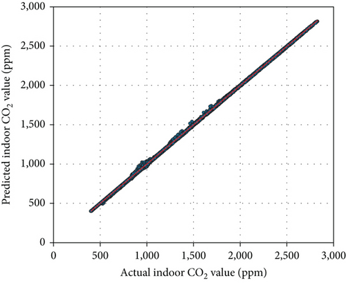
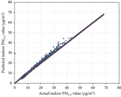
3.2. Case Studies
3.2.1. Case Definitions
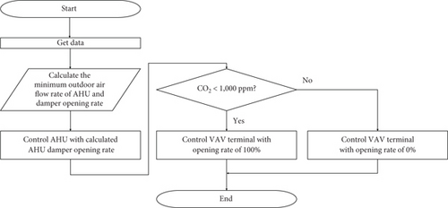
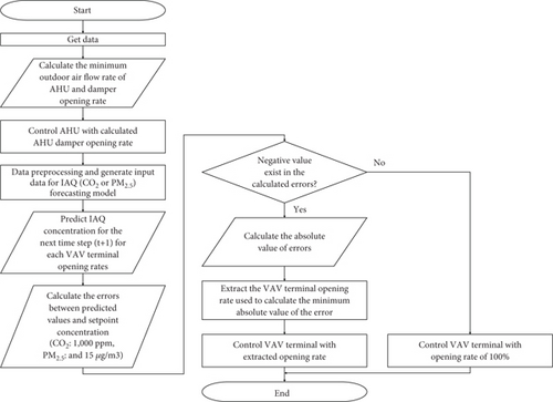
In this study, three control algorithms (Cases 1–3) were defined as comparison groups to effectively demonstrate the performance of the optimal ventilation strategy. Each control algorithm is illustrated in Figure 7. Case 1 employs the conventional ventilation control logic of the VAV system, known as DCV-CO2. This control is applied at the system level, with on–off control based on a CO2 concentration threshold of 1000 ppm applied to the VAV terminals. The positions of the VAV terminal dampers for on and off states are 0% and 100%, respectively. Case 2 combines system-level DCV-CO2 with zone-level CO2 predictive control. The CO2 prediction model is applied at the zone level, predicting CO2 concentrations at each time step and calculating errors based on the 1000 ppm threshold. If all errors are positive, the VAV terminal dampers are fully opened. If there are negative errors, the dampers are controlled to the opening rate that minimizes the absolute value of the error rate. Case 3 also applies DCV-CO2 at the system level, but at the zone level, PM2.5 predictive control, incorporating the PM2.5 prediction model, is used. The control process for PM2.5 follows the same procedure as Case 2. The threshold for PM2.5 is set at 15 μg/m3. Finally, Case 4 is the optimal ventilation strategy, which simultaneously controls both CO2 and PM2.5. A summary of each case is provided in Table 3. Simulations for performance evaluation of the control algorithms were conducted over five weekdays that were different from the period used for training the IAQ prediction models.
| Cases | Control methods | |
|---|---|---|
| AHU | VAV terminal | |
| Case 1 | DCV-CO2 | On–off control |
| Case 2 | DCV-CO2 | CO2 predictive control |
| Case 3 | DCV-CO2 | PM2.5 predictive control |
| Case 4 | DCV-CO2 | Integrated control |
3.2.2. Prediction Accuracy
The effectiveness of predictive control fundamentally depends on the accuracy of the embedded prediction models. Significant deviations in the forecasts of future environmental variables can lead to system malfunctions, resulting in uncomfortable indoor conditions. Therefore, it is crucial to assess the accuracy of these predictions rigorously. Table 4 presents the prediction accuracy metrics for each case. For Case 2, the CO2 prediction metrics were a MAE of 9.28 ppm, a CVRMSE of 1.78%, and an R2 of 0.99. For Case 3, the PM2.5 prediction metrics were a MAE of 0.16 μg/m3, a CVRMSE of 1.29%, and an R2 of 0.97. In Case 4, the CO2 prediction results yielded a MAE of 9.31 ppm, a CVRMSE of 2.16%, and an R2 of 0.99, while the PM2.5 prediction results showed a MAE of 0.16 μg/m3, a CVRMSE of 1.42%, and an R2 of 0.99. These results indicate that the prediction models performed with high accuracy across all cases, ensuring stable operation of the control systems. Figure 8 illustrates scatter plots comparing actual versus predicted values, confirming that no significant outliers were present in the predictions.
| Cases | MAE | CVRMSE | R2 |
|---|---|---|---|
| Case 2—CO2 | 9.28 ppm | 1.78% | 0.99 |
| Case 3—PM2.5 | 0.16 μg/m3 | 1.29% | 0.97 |
| Case 4—CO2 | 9.31 ppm | 2.16% | 0.99 |
| Case 4—PM2.5 | 0.16 μg/m3 | 1.42% | 0.99 |
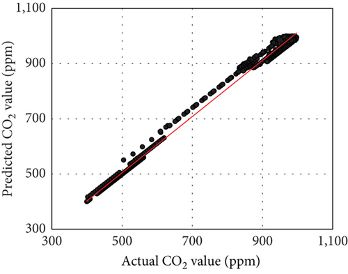
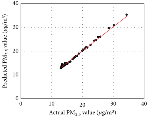
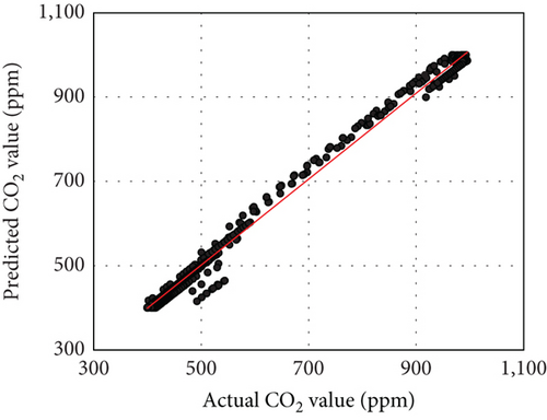
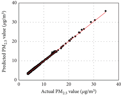
Although the prediction models demonstrate high accuracy, achieving similar accuracy in actual building applications may be challenging due to uncertainties such as external disturbances and sensor measurement instability. This can be observed in Figure 8, where relatively large discrepancies between actual and predicted values mostly occur during rapid fluctuations in CO2 and PM2.5 levels. The indoor air prediction models depend on the current occupant count as an input variable, and since CO2 and PM2.5 levels are influenced by occupants’ respiration and activity, prediction mismatches can arise without information on future occupancy changes. Anticipating occupant schedules could reduce the impact of uncertainty in real-world applications.
3.2.3. Computation Time
The computation time is critical for real-time control. In the optimal ventilation strategy, the prediction process of the indoor air models constitutes the largest portion of the computation time. Simulations were conducted on an Intel Core i5-10600 processor with 16 GB RAM, achieving computation times of less than 1 s per time step. This efficiency is attributed to the simple configuration of the prediction models and minimal input data requirements. With sufficient performance servers in actual building applications, control delays due to computation are not anticipated.
3.2.4. Comparative Analysis of IAQ
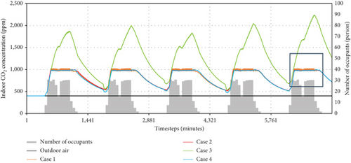
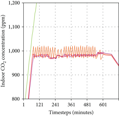
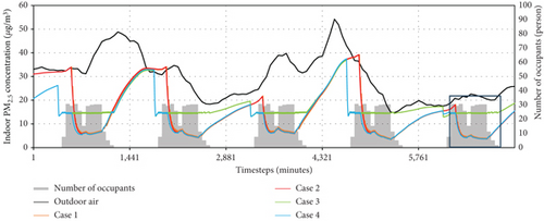
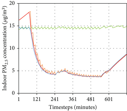
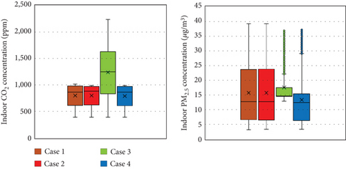
The simulation results for the four control algorithms are presented in Figures 9 and 10 and Table 5. Graphs (a) and (c) of Figure 9 display the indoor CO2 and PM2.5 concentrations for each case, respectively, while Graphs (b) and (d) offer an enlarged view for a more detailed comparison. Figure 10 shows the indoor CO2 and PM2.5 concentration distributions, and Table 5 provides the IAQ-CO2 and IAQ-PM2.5 metrics for each case.
| Cases | IAQ-CO2 | IAQ-PM2.5 |
|---|---|---|
| Case 1 | 78.38% | 89.52% |
| Case 2 | 100% | 72.57% |
| Case 3 | 23.24% | 95.33% |
| Case 4 | 100% | 97.33% |
Graph (a) indicates that for Cases 1, 2, and 4, where CO2 control criteria were established, the indoor CO2 concentrations during the control period (6:00–20:00) were maintained near the upper limit of 1000 ppm. The differences among these three cases are elucidated in Graph (b). In Case 1, the indoor CO2 concentration was higher than in Cases 2 and 4 due to the VAV terminal opening only when the CO2 concentration exceeded 1000 ppm. In contrast, the indoor CO2 concentrations in Cases 2 and 4, which utilized CO2 predictive control, remained stably below the upper limit. The minimal difference in indoor CO2 concentrations between Cases 2 and 4 suggests that CO2 control was predominantly prioritized during this period in Case 4.
Graph (c) illustrates that only in Case 3 did the indoor PM2.5 concentration approximate the upper limit, while the other cases maintained much lower concentrations than the upper limit of 15 μg/m3. This implies that CO2 had a more significant impact than PM2.5 in the given building model. Graph (d) reveals the distinctions among Cases 2, 3, and 4. Although Case 4 primarily controlled CO2 during the selected period, it maintained indoor PM2.5 concentrations below the upper limit from 6:00 to 9:30, unlike Case 2. This indicates that PM2.5 control was prioritized before the indoor CO2 concentration increased due to occupant activities. Subsequently, as CO2 control took precedence, the indoor PM2.5 concentrations in Case 4 became similar to those in Case 2. This pattern was observed not only in the zoomed area but also throughout the control period.
Unlike conventional optimization functions, the optimal ventilation strategy dynamically adjusts the target control variable in real time. Due to this approach, when the variability of one control variable is greater than the other, the VAV system may operate with a higher dependency on that specific variable. This is illustrated in Figure 10. The distribution of indoor CO2 and PM2.5 concentration in Case 4 resembles that of Cases 1 and 2, where control was primarily based on CO2. This implies that the CO2 error rate was higher than that of PM2.5 during the error rate calculation stage.
One might question whether controlling based on CO2 alone would naturally keep PM2.5 concentrations within a comfortable range. However, PM2.5 concentration is influenced by filters installed in the AHU or VAV terminals. If these filters are insufficient in removing PM2.5, its variability may increase. The control outcomes of the optimal ventilation strategy in response to this issue are discussed in further detail in Section 4.
The IAQ-CO2, representing the percentage of time the indoor CO2 concentration remained below the upper limit during the control period, was highest in Cases 2 (100.00%) and 4 (100.00%), followed by Case 1 (78.38%) and Case 3 (23.24%). This highlights the superior performance of CO2 predictive control in Cases 2 and 4. In Case 1, 21.62% of the control period experienced uncomfortable CO2 levels due to the on–off control mechanism, which only opened the VAV terminal after exceeding 1000 ppm. The low IAQ-CO2 in Case 3 indicates insufficient fresh air intake for reducing indoor CO2 levels when focusing on PM2.5 control. The IAQ-PM2.5 was highest in Case 4 (97.33%), followed by Case 3 (95.33%), Case 1 (89.52%), and Case 2 (72.57%). Despite the generally low indoor PM2.5 concentrations in Cases 1, 2, and 3 during the control period, the absence of PM2.5 control in the morning hours, when CO2 levels were low, significantly impacted the IAQ-PM2.5 results. Overall, Case 4 showed the highest comfort ratio for both control variables, indicating that the optimal ventilation strategy successfully achieved optimal control.
Comparing these results to Reference [47], IAQ-CO2 of 81.6% and IAQ-PM2.5 of 99.7% achieved by the rule-based integrated control, the optimal ventilation strategy demonstrated an 18.4% improvement in CO2 performance, although it was 2.37% lower in PM2.5 performance. However, since both studies maintained over 95% IAQ-PM2.5, it can be concluded that both approaches provide sufficiently comfortable IAQ. Although direct comparisons of relative superiority are challenging due to differing environmental, building, and system conditions between the studies, it is evident that the optimal ventilation strategy can achieve sufficiently comfortable IAQ through the optimal control of both CO2 and PM2.5.
3.2.5. Energy Usage
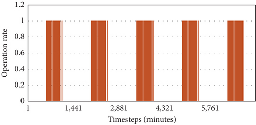
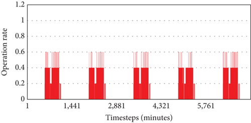
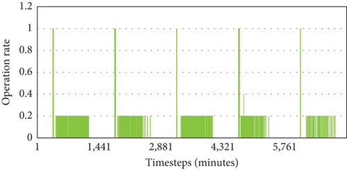
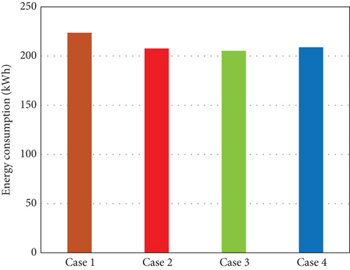
The supply airflow rate is determined by the VAV terminal opening rate, which directly impacts the supply fan energy usage. Graphs (a)–(d) in Figure 11 show the VAV terminal opening rates, while Graph (e) illustrates the fan energy usage. In Case 1, the VAV terminals fully opened when the indoor CO2 concentration exceeded the upper limit, resulting in an energy consumption of 223.65 kWh. In Case 2, as shown in Graph (b) of Figure 9, the indoor CO2 concentration was maintained below 1000 ppm with a significantly lower supply airflow rate compared to Case 1. The energy consumption in Case 2 was 207.74 kWh, reflecting a reduction of approximately 7.11% compared to Case 1. Case 3 operated with a relatively lower airflow rate compared to CO2 control, resulting in the lowest energy consumption of 205.37 kWh. Case 4 exhibited a mixed pattern of the opening rates seen in Cases 2 and 3, resulting in higher energy usage of 208.93 kWh compared to the single-variable controls but achieving a 6.58% energy reduction compared to the traditional control method in Case 1.
4. Discussions
4.1. Energy Efficiency
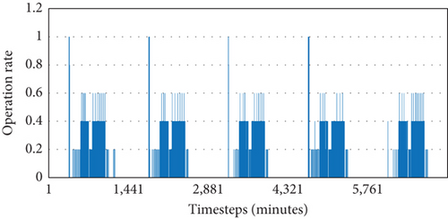
While Graphs (a)–(d) in Figure 9 initially suggest significant disparities in energy usage, the actual energy consumption did not exhibit such substantial differences. This can be attributed to the varying fan operation rates corresponding to the VAV terminal opening rates, as detailed in Table 6. Although Case 1 displayed the highest opening rates, its operation rate was the lowest at 21.52%. Conversely, Cases 2, 3, and 4, which addressed partial loads, demonstrated lower average opening rates than Case 1 but exhibited higher operation rates of 58.10%, 30.24%, and 64.27%, respectively. Among these, Case 3 achieved the lowest energy consumption due to both low opening and operation rates; however, its energy consumption was only 3.56 kWh (1.75%) less than that of the optimal ventilation strategy. These findings imply that while integrated control of multiple variables can potentially lead to increased energy consumption compared to single-variable control, the increase may not be as significant as anticipated.
| Cases | Operation rate |
|---|---|
| Case 1 | 21.52% |
| Case 2 | 58.10% |
| Case 3 | 30.24% |
| Case 4 | 64.27% |
4.2. Filter Variation
Indoor PM2.5 concentrations are significantly influenced by the performance of filters installed in the AHU or VAV terminals. Although HEPA filters can capture more than 99% of PM2.5, they may reduce the supply airflow, thereby increasing system capacity requirements and potentially compromising energy efficiency. This is particularly relevant for older HVAC systems that may not be equipped with HEPA filters. Therefore, it is crucial to compare the performance of the optimal ventilation strategy under various filtration efficiencies.
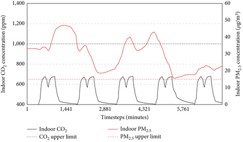
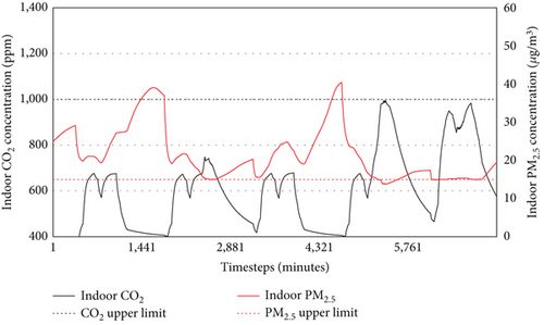
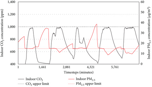
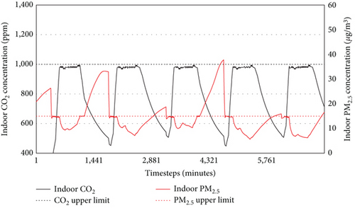
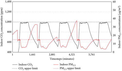
To this end, additional simulations were conducted, incrementally increasing the PM2.5 filtration efficiency from 0.0 to 0.8 in steps of 0.2, with the optimal ventilation strategy applied to all cases. Figure 12 presents the simulation results, showing indoor CO2 and PM2.5 concentrations, while Table 7 displays the operation rates for each control variable, along with IAQ metrics for each case during the control period.
| Filtration rate | Operation rate | IAQ | ||
|---|---|---|---|---|
| CO2 mode | PM2.5 mode | IAQ-CO2 | IAQ-PM2.5 | |
| 0.0 | 0.00% | 99.52% | 100% | 0.0% |
| 0.2 | 4.48% | 95.05% | 100% | 9.81% |
| 0.4 | 38.19% | 61.33% | 100% | 90.00% |
| 0.6 | 70.95% | 28.57% | 100% | 94.86% |
| 0.8 | 75.24% | 24.29% | 100% | 97.33% |
According to Figure 12, when the filter efficiency was 0.0, the system operated predominantly in PM2.5 mode, but as the efficiency increased to 0.8, the proportion of CO2 mode increased. In all cases, CO2 levels remained below 1000 ppm, and IAQ-PM2.5 improved as the filtration rate increased. For the filtration rate 0.0, although the VAV system was controlled as PM2.5 mode in most period, the IAQ-PM2.5 was 0% due to the absence of filter. The IAQ-PM2.5 of filtration 0.2 was slightly improved compared to filtration 0.0, but the filtration performance was insufficient. However, when the filtration rate changed from 0.2 to 0.4, the IAQ-PM2.5 ratio sharply increased from 9.81% to 90%, despite a high rate of switching between CO2 and PM2.5 modes. When the filtration rate increased to 0.6 and 0.8, the IAQ-PM2.5 also increased to 94.86% and 97.33%, respectively.
These results indicate that the integrated control effectiveness of the optimal ventilation strategy is maximized when filters of a certain performance level are applied. Additionally, as the filtration rate increases, the optimal ventilation strategy shows a higher tendency to prioritize CO2 control. This demonstrates that, even with varying outdoor CO2 and PM2.5 concentrations or differing rates of indoor pollutant generation and removal, the optimal ventilation strategy can consistently achieve the best possible outcomes under given conditions.
4.3. Limitations and Future Works
This study proposed an optimal ventilation strategy for VAV systems, specifically targeting air pollutants. This methodology is suitable for scenarios where only ventilation is required, such as during periods when heating and cooling are not necessary. However, during heating and cooling periods, VAV systems must concurrently manage ventilation and thermal regulation. In such instances, the rate of outdoor air intake in the AHU impacts not only the concentration of air pollutants but also the heat transfer efficiency of the heating and cooling coils, thereby directly influencing the energy consumption of chillers and boilers. Furthermore, the VAV terminals must also address the thermal comfort of occupants, necessitating the development of more sophisticated control algorithms. Consequently, future research will focus on developing integrated indoor environment control algorithms that account for both heating and cooling, enabling a comprehensive analysis of thermal comfort and IAQ.
5. Conclusions
In this study, an optimal ventilation strategy that simultaneously considers CO2 and PM2.5 was developed and evaluated. The strategy is divided into system-level and zone-level controls. At the system level, DCV-CO2 based on real-time occupant data was applied, while at the zone level, predictive control based on IAQ prediction models was implemented. This approach involved predicting indoor CO2 and PM2.5 concentrations for the next time step and dynamically adjusting the control priority based on the error rates between the predicted values and the upper limits to determine the optimal supply airflow.
- •
Ensuring the accuracy of IAQ prediction models is crucial for the stability of predictive control. In Cases 2, 3, and 4, where predictive control was applied, the CVRMSE values were all below 3%, and the R2 values exceeded 0.97, indicating high predictive accuracy. Consequently, CO2 and PM2.5 levels remained below the upper limits with minimal fluctuations throughout most of the control periods.
- •
The IAQ evaluation for Case 4, where the optimal ventilation strategy was applied, showed IAQ-CO2 at 100% and IAQ-PM2.5 at 97.33%. Compared to Case 1 (IAQ-CO2 = 78.38%, IAQ-PM2.5 = 89.52%), Case 2 (IAQ-CO2 = 100%, IAQ-PM2.5 = 72.57%), and Case 3 (IAQ-CO2 = 23.24%, IAQ-PM2.5 = 95.33%), these results demonstrate that the integrated control of CO2 and PM2.5 can reliably provide comfortable IAQ.
- •
The fan energy usage for each case was as follows: Case 1, 223.65 kWh; Case 2, 207.74 kWh; Case 3, 205.37 kWh; and Case 4, 208.93 kWh. Although the optimal ventilation strategy in Case 4 did not achieve the lowest energy consumption, the difference between Case 3 and Case 4 was a mere 1.75%. This slight difference suggests that while integrated control may improve IAQ, it could potentially increase energy usage, depending on the environment in which the optimal ventilation strategy is applied.
- •
The performance of the optimal ventilation strategy can be influenced by the presence and efficiency of PM2.5 filters in the VAV system. To verify this, tests were conducted by incrementally increasing the filtration rate from 0.0 to 0.8. When the filtration rate was 0.0, the strategy operated in PM2.5 mode 99.52% of the time, yet IAQ-PM2.5 was 0%. As the filtration rate increased, the proportion of CO2 mode also increased. Notably, when the filtration rate increased from 0.4 to 0.6, IAQ-PM2.5 surged from 9.81% to 90%, and at a filtration rate of 0.8, the performance was excellent with IAQ-CO2 at 100% and IAQ-PM2.5 at 97.33%. These results confirm that the optimal ventilation strategy can provide comfortable IAQ in environments equipped with high-efficiency PM2.5 filters.
In summary, these results demonstrate that the optimal ventilation strategy can achieve multiobjective optimal control without relying heavily on conventional optimization functions. It was also shown that, even with environmental changes, this strategy effectively maintains CO2 and PM2.5 levels within comfort thresholds. Based on the effectiveness of this approach, applying the optimal ventilation strategy to actual buildings is expected to simplify development costs and system maintenance, ultimately reducing overall building operation costs, while ensuring comfortable IAQ during non-HVAC seasons. Future research will focus on refining the control strategies to provide year-round comfort by integrating HVAC energy efficiency and occupant thermal comfort.
Conflicts of Interest
The authors declare no conflicts of interest.
Funding
This work was supported by the Korea Institute of Energy Technology Evaluation and Planning (KETEP) and the Ministry of Trade, Industry & Energy (MOTIE) of the Republic of Korea (No. RS-2021-KP002461); and this work was supported by the National Research Foundation of Korea (NRF) grant funded by the Korea government (MSIT) (No. RS-2023-00217322).
Open Research
Data Availability Statement
The datasets used or analyzed in this study may be obtained from the corresponding author upon reasonable request.


