Predicting and Analyzing Indoor Air Quality in Inpatient Wards Using IoT-Based Long-Term Data and Machine Learning
Abstract
Indoor air quality (IAQ) plays a crucial role in safeguarding the health of both patients and healthcare workers in hospital environments. Accurate IAQ analysis and prediction are vital for optimizing ventilation, filtration, and other control measures to maintain a safe indoor atmosphere. This study investigates IAQ in hospital spaces by utilizing long-term data from internet of things (IoT) sensors installed in general wards and negative pressure isolation wards. Given the significant influence of outdoor air, IAQ requires continuous monitoring across different seasons and extended periods. In this study, IAQ was measured over nearly a year, capturing seasonal variations and long-term trends. Clustering algorithms were applied to identify complex patterns and detect anomalies in key IAQ parameters, including temperature, CO2 concentration, and particulate matter 2.5 μm (PM2.5). These clustering results were then integrated into a long short-term memory (LSTM) model to enhance IAQ prediction for subsequent time steps. The findings indicate that incorporating clustering results as input variables substantially improves IAQ prediction accuracy. Notably, the root mean squared error for PM2.5 prediction decreased from 8.51 to 3.99 when clustering results were included. This study underscores the potential of leveraging IoT sensors and machine learning techniques for real-time IAQ monitoring and forecasting in hospital settings. These insights can support the development of effective control strategies to maintain a healthy and comfortable indoor environment for both patients and healthcare workers.
1. Introduction
People spend more than 90% of their time indoors. Indoor air quality (IAQ) has been a growing concern, and the COVID-19 pandemic has significantly heightened interest in this area. The COVID-19 pandemic has further heightened awareness of IAQ, particularly in healthcare settings. In response, South Korea has been expanding negative pressure isolation wards (NPIWs) to enhance pandemic preparedness. While post-COVID-19 research on negative pressure isolation rooms (NPIRs) continues, limited studies have examined their indoor environments [1]. In hospital settings, IAQ significantly impacts patient health and requires continuous monitoring [2, 3]. Regular assessment of patient rooms (PRs) is essential [4], as IAQ is primarily regulated through heating, ventilation, and air conditioning (HVAC) systems. However, verifying IAQ within PRs typically involves high-performance measurement, which creates problems such as the need to carry measurement equipment and causing inconvenience to both patients and medical staff in the ward. To mitigate these, low-cost, compact IAQ sensors offer a viable alternative. Internet of things (IoT) sensors, which have become increasingly accurate, enable continuous monitoring and remote assessment [5]. Due to advancements in IoT sensors, various studies are being conducted using IoT sensors for IAQ measurement [6–8]. This approach allows for continuous IAQ measurement by installing multiple IoT sensors to monitor IAQ in real-time across multiple locations within the wards.
IAQ forecasting is necessary for effective IAQ control [9, 10]. In PRs and NPIRs, where patients remain for extended periods, IAQ prediction is essential for timely contamination removal and health protection. By anticipating pollutant increases, HVAC systems can be proactively adjusted to control excessive concentrations [11]. For rooms with cyclical and noncyclical increases in pollutants, IAQ prediction enables more effective HVAC operation control. Even within wards, IAQ constantly fluctuates due to various activities. In PR, IAQ is subject to cyclical and noncyclical changes due to medical activities, patient activities, and changes in outside air concentration. To effectively respond to IAQ fluctuations, continuous IAQ measurement and prediction are required for each PR where the patient resides [12, 13]. IAQ prediction requires analysis of IAQ patterns, and pattern analysis requires long-term data [14]. Numerous studies have analyzed IAQ patterns in commercial, residential, and multiuse buildings [15]. Relatively few studies have been conducted in hospital settings compared to other facilities due to the difficulty of acquiring long-term data.
Machine learning is widely used to analyze large-scale IAQ data collected over an extended period [16]. Researchers have applied IoT sensor data to classify and analyze IAQ trends using unsupervised learning techniques [17, 18]. Unlike supervised learning, unsupervised learning does not rely on predefined target values; instead, it identifies patterns and clusters within datasets [19]. The learned clustering can be used to effectively divide big data according to the user’s analysis, and necessary actions can be taken accordingly for faster resolution of problems [17, 20]. By leveraging clustering techniques, daily IAQ patterns can be accurately analyzed to support performance evaluations and optimize control strategies for hospital environments [21].
This study is aimed at analyzing and predicting IAQ in hospital settings by leveraging IoT sensors to collect IAQ data within patient wards. Long-term data is utilized to assess IAQ trends in inpatient rooms, while machine learning techniques are applied to classify and analyze this data through clustering. Unlike previous studies that relied solely on environmental variables as input for the long short-term memory (LSTM) model, this study incorporates clustering results as additional input variables to enhance IAQ prediction accuracy. We compare the predictive performance of LSTM models with and without clustering integration to evaluate the impact of this approach. By leveraging these results, we aim to improve the precision of IAQ forecasting in hospital wards, ultimately supporting better air quality management strategies.
2. Literature Review
Predictions can be used to optimally vary current control parameters by forecasting whether the indoor environment will remain stable or deteriorate due to pollutant accumulation [22, 23]. Numerous studies have investigated indoor environment prediction in vulnerable facilities such as childcare centers and schools, as well as in public and commercial spaces, including libraries, classrooms, subways, and retail areas [14, 24, 25]. Yao et al. [26] applied indoor environment prediction in a residential environment and demonstrated the high accuracy of the LSTM models. Sharma et al. [27] predicted pollutant concentrations in classrooms, achieving accuracy rates of 94%–96% using LSTM models. Cho et al. [28] developed an ANN-based model for school buildings to predict indoor carbon dioxide, particulate matter 10 μm (PM10), and particulate matter 2.5 μm (PM2.5) and showed high accuracy with a root mean square error (RMSE) of 0.8816 for CO2, 0.4645 for PM10, and 0.6646 for PM2.5. However, its reliance solely on simulation results without real-world validation limited its applicability. Lee et al. [29] demonstrated effective prediction of indoor PM2.5 and PM10 using LSTM models, both in real time and 60 min into the near future, achieving 90% accuracy. Li et al. [30] demonstrated the feasibility of IAQ prediction using an LSTM model trained on data acquired from IoT sensors collected in a laboratory setting. Karaiskos et al. [31] applied an LSTM model to predict IAQ in fitness and examine its advantages. Their study incorporated IAQ data alongside occupancy levels, outdoor air conditions, and ventilation system operation to enhance prediction accuracy. Given the difficulty of obtaining occupancy rates, they predicted a graded environmental quality assessment rather than absolute values. Lu et al. [32] predicted PM2.5 concentrations in a subway environment and enhanced predictive performance by integrating the light gradient boosting machine (LightGBM) method compared to the results using the LSTM model. The model with the LightGBM method demonstrated a 20.5% reduction in RMSE compared to the simple LSTM. Kim et al. [33] predicted IAQ in daycare centers using various settings. For PM2.5 prediction, the coefficient of variation of the RMSE (CVRMSE) yielded the lowest error of 13.17% for the Bayesian regularization model. Lagesse et al. [34] predicted PM2.5 concentrations in an office with mechanical ventilation, where the LSTM model showed the lowest error, achieving an RMSE of 1.73 μg/m3. Dai et al. [35] predicted PM2.5 concentrations in a residential setting at intervals of 30 min and beyond. Using a recurrent neural network (RNN) model with an autoencoder, they reported an error of 8.3 μg/m3 for indoor PM2.5 concentrations between 20 and 50 μg/m3.
Jung et al. [36] analyzed pollutant distribution in hospital and outdoor environments based on air conditioning systems but only measured data during winter, from November to the following January. While previous research has emphasized the importance of data acquisition in hospital environments using IoT sensors, a key limitation was the collection of only 30 days of data, restricting a comprehensive analysis of IAQ variations across different seasons [5]. Zhou et al. [37] conducted IAQ prediction in a hospital outpatient hall using low-cost sensors, incorporating occupant count as an input variable derived from image data. However, this approach faces privacy concerns and requires specialized equipment, limiting its broader applicability. Additionally, their data was collected exclusively between November and January, overlooking seasonal IAQ fluctuations and reducing the generalizability of their findings. Jain et al. [38] analyzed energy performance and IAQ in urban hospital spaces, highlighting IAQ vulnerabilities in such environments. They emphasized the need for controls balancing energy consumption and IAQ. The necessity of long-term continuous IAQ monitoring was demonstrated by identifying seasonal pollutant distributions.
Previous research has extensively explored pollutant prediction in various environments, including offices, residences, and schools. However, predictive studies in hospital settings—where IAQ has the most critical impact on human health—remain limited. The constraints associated with hospital measurement spaces pose challenges in the analysis and utilization of long-term IAQ data in inpatient wards. PRs and NPIRs differ significantly from commercial and residential facilities. In commercial settings, occupancy and activity levels peak during business hours, with minimal pollutant accumulation outside of operating periods. In contrast, residential facilities are primarily occupied during nonbusiness hours, with pollutant generation mainly arising from cooking and cleaning, activities that are typically accompanied by adequate ventilation.
Hospital environments, particularly PRs and NPIRs, present unique challenges as patients remain continuously present, and contaminants are generated by both cyclical and noncyclical medical activities, in addition to general indoor activities.
In this study, IoT sensors are deployed to measure temperature, humidity, PM2.5, PM10, and CO2, collecting environmental data in general wards (GWs) and NPIWs. Long-term IAQ data is analyzed using clustering techniques, which facilitate the classification of environmental conditions. Using this dataset, we aim to predict key environmental factors—temperature, PM2.5, and CO2—through machine learning. Additionally, we propose a rapid classification and analysis method for indoor environments by applying clustering techniques to long-term IAQ data.
To enhance predictive accuracy, an LSTM model is employed to forecast indoor environmental factors by integrating clustering results as input variables. This study serves as a foundational framework for optimizing environmental control in hospital facilities. By incorporating clustering results into IAQ prediction, we aim to improve forecasting accuracy in specialized environments where outliers occur periodically. The predicted values are then utilized in conjunction with a classification model to proactively identify indoor environmental discomfort. These findings will contribute to fundamental research aimed at enhancing indoor comfort for hospital occupants.
3. Methods
3.1. IoT Sensor Configuration
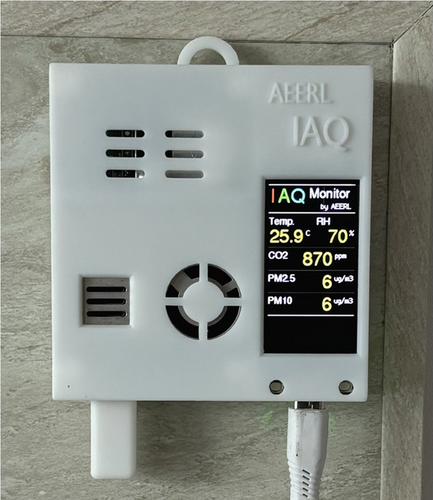
In this study, IoT sensors were employed to acquire environmental data. To assess IAQ and determine comfort levels, measurements of CO2 concentration, temperature, humidity, and particulate matter (PM) were required. Since the measurement site is continuously occupied, the sensors need to operate around the clock. To ensure uninterrupted data collection, the sensors were powered using an indoor power source for continuous monitoring. An ESP32 board with Wi-Fi functionality was used to facilitate real-time data uploading. The IoT sensor configuration was as follows: Temperature and relative humidity were measured using the Si7021-A20 sensor (Silicon Labs, United States), PM concentrations were monitored using the PM2008 sensor (Cubic, China), and CO2 levels were recorded using the CM1106-C sensor (Cubic, China). The sensor arrangement is depicted in Figure 1, while the accuracy and measurement range of each sensor are detailed in Table 1. The collected data was programmed for automatic uploading to ThingSpeak (MathWorks, United States) at 1-min intervals. For external air quality data, measurements were obtained from the closest available external monitoring station relative to the target indoor space.
| Sensor | Measurement | Measurement range | Accuracy |
|---|---|---|---|
| Si7021-A20 | Temperature | −40°C~85°C | ±0.3°C |
| Relative humidity (RH) | 5%~95% RH | ±2% RH | |
| PM2008 | PM2.5 | 0~1000 μg/m3 | ±10 μg/m3 or |
| PM10 | ±10% of reading | ||
| CM1106-C | CO2 | 0~5000 ppm | ±50 ppm or |
| ±5% of reading | |||
3.2. Data Acquisition in Inpatient Ward
The IoT sensors were installed in a ward containing both NPIRs and GWs at Medical Center A. Sensors were placed in 10 locations within the ward, specifically in the nurse station (NS), PRs of the GW, and NPIRs, as illustrated in Figure 2. Data acquisition using IoT sensors was conducted from August 16, 2023, to July 22, 2024. Of the data collected during this period, six rooms were selected for analysis, excluding data from four sensors that experienced prolonged data loss due to sensor malfunctions and upload errors. To ensure accurate data collection, sensor placement was carefully considered based on typical occupant positioning. The sensors installed in NS were installed at a height of 1.1 m from the floor, similar to the height of the respiratory tract in a seated position. In the specialized space of a hospital room, patients spend a lot of time lying down, so we install the sensors at a height of 0.8 m above the floor, which is as close to the respiratory level of a bedridden person as possible in the available space. For CO2 concentration measurements, the sensors were installed in a location that is less influenced by the direction of the airflow from the supply vent, and for temperature measurements, in a room that is not directly exposed to direct sunlight. Four unused sensors were excluded because the total amount of missing data for 3 consecutive days exceeded 3 months, which was significantly more than for other sensors. When using 10-min interval data, if data was missing at exactly 10 min, the closest data within 5 min was used. For the six sensors used, linear interpolation was used for missing data within 1 h.
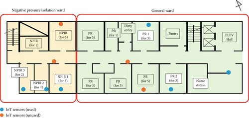
The ward is air-conditioned using the HVAC system. The system operates continuously from 06:00 to 22:00, with a scheduled noise shutdown from 22:00 to 06:00. The HVAC runs at those times at the request of the patient or at the discretion of the administrator. In PRs, the HVAC system supplies 100% outside air during patient mealtimes, while at other times, it maintains a mix of 30% outside air and 70% recirculated air. Additionally, fan coil units (FCUs) are installed near windows to provide localized cooling. PR 2, which faces southwest, is exposed to significant sunlight throughout the day. The standard room temperature is set at 24°C, with allowable adjustments of up to ±3°C depending on the patient’s condition. NPIRs maintain negative pressure relative to adjacent areas to prevent airborne contaminant leakage. A pressure differential of 1.6 Pa is maintained between the GW corridor and the NPIW corridor, while a pressure difference of approximately 3 Pa is sustained between the NPIW corridor and the NPIR to prevent contamination transfer from the NPIR to surrounding spaces.
The NS is continuously staffed, while the number of patients in each room fluctuates. Nurses operate on daily shifts at 06:30, 14:30, and 21:30. Each patient undergoes blood pressure measurements three times a day at 07:00, 15:00, and 22:00, and blood tests at 05:00 at least once a week. Hospital rooms are sanitized twice daily, once in the morning and once in the afternoon. Patients follow a structured meal schedule, with breakfast at 07:30, lunch at 12:00, and dinner at 17:30. The NPIW corridor maintains a pressure differential of approximately 1.6 Pa relative to the GW corridor, while the NPIR maintains a pressure difference of approximately 3 Pa relative to the NPIW corridor to control airborne infection leakage.
3.3. One-Day Data Clustering
To analyze daily variations in indoor IAQ data, the acquired long-term dataset was segmented into daily units, allowing for comparisons across different days within the measurement period. K-means clustering was applied to these daily data segments, utilizing both the daily mean and changes in IAQ parameters. K-means clustering is a fundamental unsupervised learning method used for data partitioning [39]. The algorithm categorizes data into K-predefined clusters by measuring the Euclidean distance between data points and cluster centroids. Initially, K cluster centers are randomly assigned. Each data point is then allocated to the nearest centroid based on Euclidean distance calculations, as shown in Equation (1). Once data points are grouped, the centroids are recalculated by averaging the data within each cluster. This process is iteratively repeated until the centroids stabilize and no longer change. K-means clustering is computationally efficient and straightforward to implement. However, it has inherent limitations: The number of clusters (K) must be predefined, and the algorithm’s performance is highly sensitive to this choice. Selecting an appropriate K value can be challenging, as K-means assumes that clusters have circular distributions, making it less effective for datasets with complex structures.
3.4. Outlier Identification Method Using the Entire Data
Outlier identification is essential for refining IAQ data measurements and ensuring their effective integration into predictive models. Rather than defining outliers using predefined numerical thresholds, we employ a clustering-based approach to analyze all data points. To detect outliers, the Hierarchical Density-Based Spatial Clustering of Applications with Noise (HDBSCAN) model is utilized. HDBSCAN is a density-based clustering algorithm that identifies clusters by detecting regions of high data density while treating low-density areas as noise [40]. This approach offers several advantages: It automatically determines the optimal number of clusters, accommodates various cluster shapes, and efficiently handles noise. However, compared to K-means and Gaussian mixture models, HDBSCAN has a higher computational complexity. Additionally, clustering outcomes are highly sensitive to hyperparameter settings, requiring careful tuning and an in-depth understanding of these parameters. HDBSCAN determines the k-nearest neighbor distance of each data point using Equation (1), as referenced in Equation (2), and calculates the relative density of the dataset. Based on this density estimation, it computes the mutual reachability distance, as expressed in Equation (3). The algorithm then constructs a minimum spanning tree (MST) by connecting closely related points within each cluster. Hierarchical clustering is applied to merge or separate clusters based on density-based connectivity. The final cluster selection is determined by identifying the cluster with the highest stability, ensuring robust outlier detection and classification.
3.5. IAQ Prediction Using LSTM
LSTM models demonstrate outstanding performance in time series data prediction in various fields. LSTM models are used in combination with various other models [41–43]. The LSTM model is employed to predict IAQ, specifically forecasting PM2.5, CO2 concentration, and temperature 10 min in advance. To facilitate this prediction, data recorded at 1-minute intervals is segmented into 10-min intervals, and the historical reference range is set to 144 data points per day. LSTM is RNN architecture designed to capture temporal dependencies in time series data, making it well-suited for IAQ prediction. Unlike standard RNNs, LSTM includes specialized memory units—referred to as memory blocks—at each hidden node, which regulate the flow of information through three types of gates: input gate, output gate, and forget gate [44]. These gates control the retention, updating, and removal of information, thereby addressing the issue of vanishing gradients commonly found in conventional RNNs. The input gate determines how much of the new input information is integrated into the model’s state, as shown in Equation (4). The output gate modulates the output value stored in the model’s internal state, as shown in Equation (5). The forget gate decides how much of the previous state’s information should be retained at the current time step, as expressed in Equation (6). As information progresses through the forget gate, portions of long-term memory are discarded, while new memory is incorporated via the input gate. This results in a dynamically updated long-term state, which is directly output at each time step. The short-term state is derived from this long-term state and processed through the output gate to generate the final node output. The neural network learns to selectively retain, discard, and retrieve specific parts of the long-term state for optimal predictions.
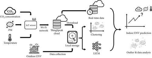
This study is aimed at collecting and utilizing long-term data from NPIR and GW, which are specialized indoor environments. The long-term IAQ dataset is analyzed using clustering techniques to detect and classify outliers. Based on this analysis, key factors influencing IAQ prediction are identified, and the clustering results are integrated into the LSTM model to assess whether prediction accuracy improves. Figure 3 presents the overall workflow of the research project.
4. Result
4.1. Analysis of the Long-Term IAQ Data
IAQ data from 6 of the 10 monitored spaces were analyzed using IoT sensors. Four sensors were excluded due to persistent data loss or measurement errors caused by sensor malfunctions or upload failures, leading to more than 1 day of missing data. The remaining six sensors exhibited minor short-term data gaps, which were addressed using linear interpolation to estimate the missing values. Figure 4 illustrates the 24-h IAQ data trends for the monitored spaces over the measurement period.
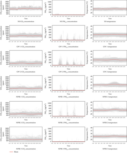
Temperature data were collected from a hospital environment, where the indoor climate is regulated by an HVAC system. Table 2 presents the mean and standard deviation for each monitored space, providing a summary of the overall temperature distribution. Across all monitored spaces, the annual average temperature ranged between 25°C and 26°C, with the set temperature maintained at 24°C. The temperature remained within the target range of 21°C–27°C for most of the observation period. However, between 2:00 and 4:00 PM, the average temperature consistently increased across all measurement points except for PR 1. This temperature discrepancy is likely attributed to the hospital’s geographical location in the northern hemisphere, where all rooms except PR 1 face south and are exposed to direct sunlight during the afternoon, leading to elevated indoor temperatures.
| Temp (°C) | CO 2 (ppm) | PM2.5 (μg/m3) | ||
|---|---|---|---|---|
| Nurse station | Mean | 26.68 | 1000 | 12.73 |
| Standard deviation | 1.23 | 73.07 | 7.34 | |
| PR 1 | Mean | 25.94 | 791 | 9.76 |
| Standard deviation | 1.44 | 94.19 | 16.38 | |
| PR 2 | Mean | 25.65 | 520 | 15.64 |
| Standard deviation | 1.63 | 83.74 | 28.02 | |
| NPIR 1 | Mean | 26.12 | 519 | 9.80 |
| Standard deviation | 1.36 | 75.94 | 10.37 | |
| NPIR 2 | Mean | 26.87 | 546 | 10.49 |
| Standard deviation | 1.12 | 98.63 | 18.47 | |
| NPIR 3 | Mean | 25.66 | 523 | 9.16 |
| Standard deviation | 1.19 | 87.16 | 6.35 | |
Table 2 indicates that NPIR 1 recorded multiple instances where temperatures exceeded 30°C. This phenomenon can be attributed to the FCU being turned off when the room is unoccupied. In the NS room, the temperature remained relatively higher compared to other monitored spaces, likely due to two primary factors: (1) the presence of a false partition wall, which separates the room from the FCU, limiting airflow, and (2) the continuous operation of various medical and electronic equipment, which generates additional heat. Additionally, slight temperature increases were consistently observed at 07:00, 15:00, and 22:00, likely coinciding with increased occupancy levels during nurse shift changes.
Regarding CO2 concentration, most rooms—except for NS—maintained levels below 1000 ppm. In the NS room, daily average CO2 levels exhibited periodic increases at 06:00, 14:00, and 22:00, mirroring the temperature trends. This pattern is likely linked to increased occupancy during nurse shift transitions. Across all monitored rooms, CO2 concentrations consistently spiked around 07:00 for approximately 1 h, which can be attributed to the daily medical checkups conducted immediately following the shift changes. These activities involve increased movement and interaction between patients and healthcare staff, leading to temporary elevations in CO2 levels.
For PM, all monitored spaces recorded values below 20 μg/m3, indicating generally low PM levels. However, the standard deviation was significantly higher in PRs, except for NS. As illustrated in Figure 4, PM2.5 levels exhibited sharp increases at 06:00, 12:00, and 17:00, leading to higher fluctuations. During these periods, PM2.5 concentrations exceeded 1000 μg/m3, a value substantially higher than outdoor levels, suggesting that the spikes were primarily caused by indoor activities rather than external influences. The average and standard deviation of PM levels were lower in NPIR rooms compared to PR rooms, which can be attributed to the additional exhaust system in NPIR rooms designed to maintain negative pressure. This system effectively enhances pollutant removal, reducing PM accumulation more efficiently than in PR rooms.
4.2. Long-Term IAQ Clustering Results
The clustering analysis was conducted using two approaches. First, the dataset was segmented into daily intervals, and for each day, key statistical features, including the daily average, daily maximum, mean of daily instantaneous changes, and daily standard deviation, were calculated and used as clustering parameters. Second, clustering was performed at the individual data point level using both indoor and outdoor indicators from the complete dataset. The elbow method and silhouette analysis were used to determine K, the optimal number of clusters for K-means clustering. For the 1-day data, K was determined to be 3. For HDBSCAN, multiple combinations of minimum cluster size and minimum sample size were tested to ensure accurate classification. For clustering based on all data points, the minimum cluster size was set to 1000, while the minimum sample size was set to 100. Since the dataset was collected from three distinct spaces, NS, PR, and NPIR, the clustering results for each space were compared to assess variations.
Figure 5 presents the clustering results for K-means applied to 1-day temperature data and HDBSCAN applied to the entire dataset. The K-means clustering analysis grouped the NS, PR, and NPIR spaces into three clusters: Cluster A represented days with relatively high indoor temperature variability. The distribution of days in Cluster A was 98 days in NS, 52 days in PR, and 20 days in NPIR out of 342 monitored days. Most of these days fell between November and February when outdoor temperatures ranged from −10°C to 5°C. During this cold period, HVAC operations induced periodic indoor temperature fluctuations between 24°C and 26°C. In NS, temperature variations were more pronounced due to its proximity to the elevator hall and the front desk, both of which influenced thermal conditions. Cluster B comprised 135 days in NS, 164 days in PR, and 137 days in NPIR. This cluster exhibited stable indoor temperatures ranging from 25°C to 28°C, primarily occurring between February and May and in part of October when demand for heating or cooling was minimal. Cluster C included 109 days in NS, 126 days in PR, and 185 days in NPIR. This cluster was primarily observed during the summer months of June to August and in part of October, where cooling operations maintained indoor temperatures between 23°C and 25°C.
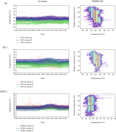
The HDBSCAN results revealed the presence of outlier regions, which appear as unclustered purple points in Figure 5. These outliers were identified in NS, PR 2, and NPIR 2, where indoor temperatures deviated significantly from expected values, particularly when outdoor temperatures ranged between −5°C and 5°C. A notable outlier was detected in NPIR, where indoor temperatures reached nearly 40°C on a day when outdoor temperatures exceeded 30°C. This anomaly may have occurred due to FCU inactivity during room vacancy, even though the sensor was positioned away from direct sunlight. However, further investigation is required to confirm this hypothesis.
For CO2 concentration, most monitored rooms—excluding NS—maintained levels below 1000 ppm. In NS, daily average CO2 concentrations exhibited increases at 06:00, 14:00, and 22:00, following a pattern similar to temperature variations. These fluctuations were likely caused by increased occupancy during nurse shift changes. Across all rooms, CO2 levels spiked around 07:00 for approximately 1 h, most likely due to daily medical checkups conducted immediately after shift changes, leading to heightened indoor activity among patients and healthcare staff.
Regarding PM2.5, all monitored spaces recorded concentrations below 20 μg/m3. However, PRs, except NS, exhibited significantly higher standard deviations. As illustrated in Figure 4, PM2.5 levels displayed sharp increases at 06:00, 12:00, and 17:00, contributing to elevated standard deviations. During these periods, PM2.5 concentrations exceeded 1000 μg/m3, far surpassing outdoor levels, suggesting that these spikes were likely induced by indoor activities rather than external influences. The average and standard deviation of PM levels were lower in NPIR rooms compared to PR rooms, likely due to the additional exhaust system in NPIR rooms, which maintains negative pressure and enhances pollutant removal efficiency.
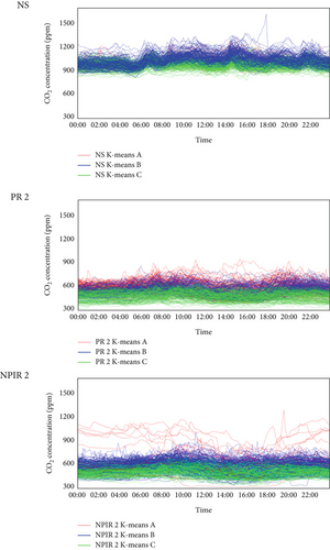
The K-means clustering results for 1-day CO2 concentration data are shown in Figure 6. In the NS space, where staff operate continuously in three shifts, the average CO2 concentration was the highest, with minimal variation, as observed in Table 2. Clusters A, B, and C in NS exhibited similar characteristics with no significant deviations. In PR and NPIR spaces, conditions where CO2 concentrations consistently ranged between 600 and 800 ppm were classified as Cluster B, while conditions where CO2 levels remained below 600 ppm were grouped into Cluster C. Regardless of the season, CO2 concentrations showed a tendency to remain elevated for periods lasting from 3 to 14 days or, conversely, remained low for several consecutive days. These fluctuations suggest that variations in CO2 levels were influenced by patient occupancy in the rooms.
The K-means clustering results for the 1-day data using PM2.5 concentration data and the HDBSCAN results for the entire dataset are shown in Figure 7. Using the 1-day data, the K-means model classified the NS, PR, and NPIR spaces into three clusters.
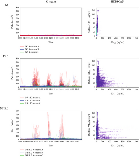
Cluster A represented days with average concentrations ranging from 25 to 30 μg/m3, characterized by higher peak concentrations and significant variations. This cluster included 38 days in NS, 99 days in PR 2, and 11 days in NPIR 2 out of 342 monitored days. In NS, PM2.5 concentration changes were relatively minimal, with a maximum recorded concentration of 76 μg/m3, which was lower compared to other spaces. In NPIR 2, peak concentrations were generally higher during the day than in PR 2, although the frequency of sharp increases was relatively low. PR 2, as seen in Table 2, had the highest mean and standard deviation for PM2.5 concentration, with Cluster A being more prevalent in PR 2 than in other spaces. In most monitored spaces, including PR 2, peaks were observed at 6:00, 12:00, and 16:00. However, PR 2 also exhibited a notable peak at 21:00, and one peak was recorded at 01:00 on a single day. The periodic nature of peak concentrations suggests that these increases were likely associated with room disinfection, patient meals, patient activities, medical rounds, and blood pressure measurements.
Cluster B represented days with moderately elevated peak concentrations and average daily concentrations between 15 and 25 μg/m3. This cluster comprised 112 days in NS, 32 days in PR 2, and 39 days in NPIR 2. In PR 2, the frequent occurrence of peak events resulted in fewer days being classified under Cluster B, while NPIR 2 exhibited lower overall daily concentrations, leading to a higher proportion of days in this cluster.
In NS, due to its direct connection with the ELEV Hall, PM2.5 concentrations were more susceptible to outdoor influences. Additionally, continuous nurse activity contributed to higher concentrations, resulting in NS having the largest number of 1-day data points among the three spaces.
Cluster C represented days with average concentrations ranging from 10 to 15 μg/m3, comprising 192 days in NS, 209 days in PR 2, and 292 days in NPIR 2 out of 342 monitored days. In NPIR 2, as a specialized NPIR, a continuous exhaust ventilation system was employed to control contaminant release, resulting in very low PM2.5 concentrations on 292 days, which accounted for 85% of the total measurement period.
The HDBSCAN clustering results, applied to the entire dataset for NS, PR 2, and NPIR 2, are also shown in Figure 7. Points represent data not assigned to any cluster. In PR 2 and NPIR 2, sudden increases in indoor PM2.5 concentrations were identified as outliers, regardless of outdoor PM2.5 levels, highlighting the impact of indoor activities. Rather than using predefined PM2.5 thresholds for outlier detection, the HDBSCAN-based anomaly detection method identified abnormal indoor PM2.5 concentrations while accounting for the distinct characteristics of each monitored space. Additionally, clusters formed based on indoor PM2.5 levels were distinguishable according to their specific concentration ranges.
4.3. IAQ Prediction Results
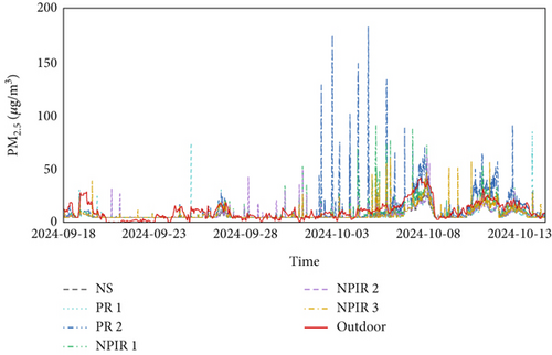
Using data collected from August 16, 2023, to July 22, 2024, an LSTM model was employed for IAQ predictions. To validate the model’s accuracy, unseen data from September 17, 2024, to October 14, 2024, which were not used during training, were utilized. The model processed 10-min interval data to forecast environmental conditions 10 min ahead, using the preceding 144 data points as input. The prediction results, compared with actual values, are presented in Table 3. Predictions were made for temperature, PM2.5 concentration, and CO2 concentration across all monitored spaces. Figure 8 presents the validation period data for each ward room, along with outdoor data. The PM2.5 concentration changed rapidly in multiple wards during this period, making it an appropriate period for verification during a continuous period. Therefore, verification was conducted using data from this period. During this period, from October 5 onward, outdoor PM2.5 concentration exhibited an increasing trend compared to previous days. Notably, the PM2.5 concentrations measured inside the ward followed a similar trend to the outdoor PM2.5 levels, indicating a possible influence of outdoor air quality on IAQ conditions. For PM2.5 predictions, comparisons were performed using Case 2, which included outdoor concentration as an additional input variable. Further comparisons were conducted with Case 3 and Case 4, where HDBSCAN and K-means clustering results were incorporated as additional input features to evaluate their impact on prediction accuracy.
| Temp (°C) | CO2 (ppm) | PM2.5 (μg/m3) | |||||
|---|---|---|---|---|---|---|---|
| Case 1 | Case 2 | Case 3 | Case 4 | ||||
| NS | RMSE | 0.35 | 96.16 | 1.74 | 0.68 | 0.45 | 1.21 |
| CVRMSE (%) | 1.17 | 19.19 | 24.71 | 9.722 | 6.416 | 17.26 | |
| PR 1 | RMSE | 0.33 | 113.22 | 3.09 | 1.57 | 1.08 | 1.56 |
| CVRMSE (%) | 1.31 | 22.82 | 41.42 | 21.11 | 14.54 | 20.98 | |
| PR 2 | RMSE | 0.66 | 45.88 | 8.51 | 4.76 | 3.99 | 6.28 |
| CVRMSE (%) | 2.68 | 8.76 | 70.21 | 39.30 | 32.91 | 51.80 | |
| NPIR 1 | RMSE | 0.33 | 65.68 | 3.51 | 2.32 | 1.86 | 2.03 |
| CVRMSE (%) | 1.21 | 12.62 | 43.44 | 28.78 | 22.97 | 25.17 | |
| NPIR 2 | RMSE | 0.34 | 53.60 | 4.60 | 2.39 | 1.89 | 12.07 |
| CVRMSE (%) | 1.29 | 11.79 | 49.38 | 25.69 | 20.34 | 129.52 | |
| NPIR 3 | RMSE | 0.12 | 25.36 | 2.83 | 1.58 | 1.09 | 1.36 |
| CVRMSE (%) | 0.44 | 4.87 | 36.20 | 20.20 | 13.91 | 17.34 | |
For temperature predictions, the RMSE across all spaces was below 1, indicating minimal error. Since the monitored spaces are hospital wards occupied by patients, IAQ is continuously monitored and managed. Temperature regulation is maintained through HVAC and FCU systems, ensuring optimal conditions. Due to the high thermal inertia of indoor temperature, which requires significant energy input to change and typically exhibits only minor variations over short timeframes, RMSE values remained low. Among the monitored spaces, PR 2 had the highest RMSE (0.66), while NPIR 3 had the lowest RMSE (0.12). Figure 9 presents a comparison of predicted versus actual temperatures for these two spaces. In PR 2, which exhibited larger prediction errors, significant daily temperature variations were observed over the month. In contrast, NPIR 3, which had the lowest RMSE, exhibited minimal daily temperature fluctuations, with temperature changes not exceeding 3°C throughout the month. This temperature stability in NPIR 3 is attributed to the continuous operation of the ventilation system. Additionally, since patients remained present in the NPIR throughout the study period, daily temperature variations were reduced, ensuring a more stable indoor environment.

For CO2 concentration, the HVAC system continuously managed IAQ, maintaining CO2 levels around 500 ppm due to the controlled nature of the monitored spaces. The lowest RMSE was recorded in NPIR 1 (25.36), while the highest RMSE occurred in PR 1 (113.2). Figure 10 presents a comparison of predicted versus actual CO2 concentrations for PR 1 and NPIR 1. From the graph, it is evident that while the model for PR 1 followed the overall trend, it consistently predicted CO2 concentration values that were offset by approximately 100 ppm, leading to higher errors. In contrast, NPIR 1 exhibited minimal deviation between predicted and actual values, resulting in lower RMSE. However, on October 8 at 8:50 AM, a sudden increase in actual CO2 concentration was observed, rising to 915 ppm from 673 ppm in the previous time step at 8:40 AM. For approximately 1 h following this spike, the sensor failed to properly record PM2.5, temperature, and CO2 data. This suggests that during user manipulation of the sensor, CO2 concentration may have risen sharply due to exhalation.

For PM2.5 concentration, significant differences in RMSE were observed across different rooms. As indicated in the previous indoor environmental data analysis, PM2.5 concentrations exhibited substantial increases at specific times of the day. Consequently, the RMSE for PM2.5 predictions was higher compared to temperature predictions. The lowest RMSE for PM2.5 predictions was recorded in NS (1.74), whereas the highest RMSE was observed in PR 2 (8.51). Figure 11 presents a comparison between predicted and actual values in PR 2 and NS. As evident from the data analysis, NS did not exhibit the periodic increases in PM concentration observed in other PRs. Predictions for NS, a space showing gradual changes in PM2.5 concentration, had a low CVRMSE of 24.71%, indicating higher prediction accuracy. In contrast, PR 2 exhibited the most frequent periodic increases in PM2.5 concentration among all monitored rooms. These fluctuations were also observed in the validation data, contributing to higher prediction errors.

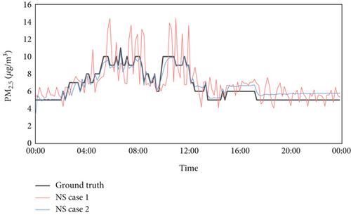
In Case 2, which incorporated outdoor PM2.5 concentration as an additional input variable, prediction accuracy improved across all spaces. Specifically, in NS, where sharp changes in PM2.5 concentration were not observed, RMSE decreased from 1.74 to 0.68, demonstrating enhanced accuracy. Additionally, RMSE was reduced by up to 33.8% (from 0.68 to 0.45), depending on whether HDBSCAN was applied. Figure 12 presents a comparison of the predicted and actual PM2.5 values for a single day in NS for Case 1 and Case 2. While Case 1 followed the overall trend of PM2.5 concentration changes, it exhibited significant fluctuations. In contrast, Case 2, which included outdoor PM2.5 concentration as an input variable, better captured the influence of outdoor air quality on indoor background concentrations, leading to fewer fluctuations compared to Case 1. Although both cases followed the overall trend, fluctuations in predicted values were reduced in Case 2, resulting in improved accuracy across all spaces.
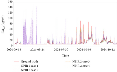
To account for sharp increases in PM2.5 concentration, clustering results were incorporated into the LSTM model for training and validation. Based on the input variables from Case 2, Case 3 included HDBSCAN clustering results derived from PM2.5 concentration and outdoor PM2.5 concentration as additional input variables, while Case 4 used K-means clustering results as additional inputs. As shown in Table 3, the results of Case 3 demonstrated reduced errors compared to Case 2 across all rooms. In particular, in PR 2, which had the highest error in Case 1 with an RMSE of 8.51, the RMSE decreased to 3.99 in Case 3. PR 2 experienced rapid PM2.5 concentration increases, and incorporating the HDBSCAN model effectively classified noise, allowing the LSTM model to better capture these fluctuations during training and validation. This led to a comparatively lower prediction error in Case 3. However, Case 4 showed significantly higher errors in NPIR 2. As shown in Figure 13, on September 22, Case 4 predicted a very high PM2.5 concentration, whereas the actual PM2.5 concentration remained very low.
5. Discussion
5.1. IoT and Machine Learning to Improve Ward IAQ
In South Korea, IAQ management standards for healthcare facilities require that the daily average PM2.5 concentration remains below 35 μg/m3 in healthcare and elderly care facilities [45]. The WHO recommends a stricter standard of 15 μg/m3 or less, which is lower than the regulations set by many countries, including South Korea [46]. Several other countries suggest maintaining an average PM2.5 concentration between 20 and 40 μg/m3 per day. As shown in Table 2, the average PM2.5 concentrations during the measurement period did not exceed 20 μg/m3 in any monitored space. While PM2.5 levels were consistently maintained within acceptable limits, occasional high-concentration peaks were observed, indicating the need for additional management measures. These peaks are difficult to detect using traditional testing methods. However, IoT sensors offer a solution by continuously acquiring IAQ data in hospital wards, enabling more effective air quality management. Through clustering, the risk level for each period is predicted based on the satisfactory pollutant concentration levels during the entire average period, and improvements to the existing standards are considered. By using IoT-based continuous monitoring, IAQ management can be enhanced, and the large volume of acquired data can be further utilized through machine learning applications. In this study, IoT sensors used external network Wi-Fi to transmit data to the outside for research. For this reason, four sensors had missing values due to Wi-Fi connection errors, and there were many periods of more than 3 days, so they were excluded for continuous analysis. This could be reduced by using an internal network connection method or acquiring data locally through a wired connection. In addition, CFD and machine learning could be used to identify sensor locations that are representative of the room, and multiple sensors could be installed to minimize missing data due to sensor errors [47]. When employing clustering models for data analysis, it is essential to consider the characteristics of each model. The performance of clustering models can vary based on the distribution of the data, which affects the accuracy and relevance of clustering results. To obtain meaningful classifications, it is necessary to evaluate the algorithms used by each model and select the most appropriate method based on data characteristics. K-means clustering is advantageous for easily identifying data characteristics through cluster centroids, making it useful for analyzing indoor environmental data. In contrast, HDBSCAN clustering identifies data points that do not belong to any specific cluster based on data density, allowing for more effective detection of outliers. This capability makes HDBSCAN particularly useful for identifying abnormal IAQ patterns that may otherwise be overlooked in standard analyses [48].
Previous studies have been limited in their ability to predict indoor environments and conduct clustering analyses using hospital data. Many studies have relied on data collected during specific periods; however, there is a need for research utilizing datasets that capture seasonal variations over an entire year. A 1-month measurement period is insufficient to account for changes in outdoor temperature and PM concentrations across different regions. To comprehensively analyze IAQ, it is necessary to collect and monitor long-term data for over a year [38]. In this study, clustering analysis of temperature, humidity, and PM2.5 concentrations revealed that certain months were dominant in each clustering result, a pattern that could only be identified through long-term measurements. Long-term IAQ monitoring enables seasonal, monthly, and daily trend analyses, highlighting that during periods of significant fluctuations in temperature, humidity, and PM2.5 concentrations, it is essential to implement more precise control strategies for each IAQ parameter. In particular, while the need for NPIW has increased significantly following COVID-19, fewer studies have analyzed indoor environmental data in NPIW compared to other types of buildings. NPIW and GW exhibit distinct characteristics from other indoor spaces, and these differences must be reflected in data analysis to ensure accurate IAQ management. Continuous IAQ data can be analyzed using machine learning and leveraged to share real-time IAQ insights with patients and medical staff in hospital wards. Based on the findings of this study, IAQ prediction and analysis can be used to enhance IAQ management by providing reliable, real-time IAQ data to ward occupants, fostering a more comfortable and healthier hospital environment.
5.2. Predicting IAQ on Wards
In hospital wards, patients engage in various indoor activities, and periodic events such as medical rounds, health assessments, and disinfection procedures influence IAQ. Analyzing environmental changes caused by these recurring events is essential for effective IAQ prediction and control. Events occurring within a ward can introduce outliers, which pose challenges to IAQ prediction by reducing model accuracy. By utilizing IoT sensors and clustering methods, real-time IAQ classification becomes possible, allowing for outlier detection and improved prediction accuracy. When employing LSTM models for IAQ prediction, incorporating clustering results as input variables enhances model performance, particularly in spaces prone to anomalies. Clustering reduced the prediction error from 8.51 to 3.99 μg/m3 in PR 2, where the mean PM2.5 concentration was 15.64 μg/m3 with a standard deviation of 28.02 μg/m3. Figure 8 shows that the background concentration of PM2.5 in the spaces within the ward follows the outdoor PM2.5 concentration. Table 3 shows that adding outside PM2.5 concentration as a prediction input variable improved the accuracy in all spaces. Indoor PM2.5 concentrations are significantly affected by outdoor PM2.5 concentrations. When predicting indoor PM2.5 concentrations, incorporating outdoor PM2.5 concentrations improves prediction accuracy. There are various studies that predict outdoor PM2.5 concentrations [43, 49, 50]. It is considered that incorporating outdoor PM2.5 concentration prediction values as additional input variables using various outdoor PM2.5 prediction models could enhance accuracy.
A previous study achieved a 54% improvement in model performance by incorporating occupancy data as an input variable [37]. However, occupancy data is often limited in availability and requires high-performance computing resources for processing, making its implementation more challenging in real-time hospital settings. In contrast, this study utilized HDBSCAN to predict IAQ based on the LSTM model, achieving a 33.4% improvement in model performance without incorporating occupancy data. The error in Case 4 with K-means as an additional input variable in Table 3 is higher than that in Case 3 with HDBSCAN as an input variable because K-means utilizes daily variation for classification and is less responsive to real-time data changes. As a result, the accuracy of Case 4 is lower than that of Case 3 because the K-means model has a harder time classifying indoor PM2.5 concentrations that increase rapidly over a short period of time than HDBSCAN. Previous studies have employed LSTM models without forgetting gates to predict PM2.5 concentrations, resulting in an RMSE of at least 1.0 [27]. RMSE was reduced by 20.5% using the LightGBM method; however, in this study, applying HDBSCAN further reduced RMSE by up to 33.8% compared to the conventional LSTM model [32]. A previous study that relied solely on the LSTM model reported an RMSE of 1.73 when predicting relatively small fluctuations in PM2.5 concentration in a mechanically ventilated office space [34]. In comparison, the LSTM model incorporating HDBSCAN achieved a significantly lower RMSE of 0.45. These results indicate that incorporating HDBSCAN into long-term IAQ prediction models can substantially improve accuracy, particularly in environments with both periodic and nonperiodic pollutant fluctuations.
One limitation of this study is the lack of data on patient occupancy within the ward. In PRs with patients, PM2.5 concentration periodically increases due to patient activity and medical procedures. However, it remains unclear how these increases correlate with the number of patients in PRs and how long peak concentrations persist. In the case of hospital wards, patients are periodically admitted and discharged, and the number of occupants fluctuates due to the movement of medical staff for medical procedures. Although there are admission and discharge schedules and medical procedure schedules, the data is not accurate daily and is difficult to reflect in real time, so this study did not use changes in the number of occupants as an input variable. Additionally, while HVAC systems were continuously operated, the set temperature and outdoor air intake rate were frequently adjusted based on patient conditions, introducing variability in IAQ data. For more accurate IAQ predictions, future research should track HVAC adjustments alongside environmental factors. Further studies should also consider patient schedules, occupancy levels, and length of stay within the monitored spaces to enable more precise data analysis and better model performance.
6. Conclusion
- 1.
Temperature and CO2 concentrations in hospital spaces were maintained within a comfortable range due to continuous HVAC operation. However, PM2.5 concentrations exhibited rapid increases, often exceeding 200 μg/m3, due to medical procedures, patient activities, and indoor disinfection processes.
- 2.
Long-term IAQ data collection using IoT sensors, combined with clustering analysis and LSTM-based predictions, enables the provision of real-time IAQ analysis and forecasting. This information can be shared with patients and medical staff, contributing to a more comfortable and healthier indoor environment.
- 3.
Incorporating clustering results as input variables in the LSTM model significantly improved IAQ prediction accuracy, particularly in spaces with periodic anomalies. This approach reduced RMSE from 8.51 to 3.99, demonstrating the effectiveness of clustering-enhanced LSTM predictions.
This study demonstrated the benefits of long-term IAQ monitoring and the use of LSTM models for IAQ prediction in hospital spaces characterized by various dynamic activities. The integration of clustering methods to detect anomalies further enhanced prediction accuracy, allowing for more precise IAQ forecasting and control strategies.
The findings of this research can be applied to optimize IAQ management, enabling proactive adjustments in hospital wards to maintain a comfortable and healthy indoor environment for patients and medical staff. This study contributes to the development of optimal control strategies for IAQ improvement, reinforcing the importance of data-driven IAQ analysis and prediction in healthcare settings.
Conflicts of Interest
The authors declare no conflicts of interest.
Author Contributions
Jehyun Kim: writing—original draft, writing—review and editing, formal analysis, methodology, software, validation, investigation, data curation, visualization, resources; Seongmin Jo: writing—review and editing; Gihoon Kim: writing—review and editing; Ji-Hi Kim: writing—review and editing; Minki Sung: writing—review and editing, conceptualization, validation, supervision, project administration, funding acquisition. All authors have read and agreed to the published version of the manuscript.
Funding
This work was supported by the Korea Institute of Energy Technology Evaluation and Planning (KETEP) and Ministry of Trade, Industry and Energy (MOTIE) of the Republic of Korea, RS-2021-KP002461, and the Infectious Disease Medical Safety funded by the Ministry of Health and Welfare, Republic of Korea, HG22C0017.
Acknowledgments
This work was supported by a grant of the project for Infectious Disease Medical Safety funded by the Ministry of Health and Welfare, Republic of Korea (grant number: HG22C0017) and by the Korea Institute of Energy Technology Evaluation and Planning (KETEP) and the Ministry of Trade, Industry and Energy (MOTIE) of the Republic of Korea (No. RS-2021-KP002461).
Open Research
Data Availability Statement
The data that support the findings of this study are available from the corresponding author upon reasonable request.


