Edge-Docker–Based Architecture for Intelligent Indoor Air Quality Management With Sensing Calibration and Automatic Controlling
Abstract
Reports show that poor indoor air quality can be harmful to vulnerable groups and lead to various health problems. To address this problem, this work proposes a management architecture for enhancing indoor air quality by integrating the analytical learning models and regulation of indoor and outdoor pollutant concentrations, which coordinates the activation or deactivation of the pollutant control devices. The proposed system incorporates predictive and calibration functionalities to enhance overall system stability and effectiveness. This work tests the prediction accuracy of multilayer perceptron and recurrent neural network models. The experimental results show that the bidirectional long short-term memory (Bi-LSTM) with a land use regression (LUR)–based feature extraction model achieves the best predictive performance with a mean absolute error of 5.74 and a mean absolute percentage error of 15.7%, respectively. Comparing the existing Bi-LSTM work for PM2.5 prediction, the proposed Bi-LSTM model with feature selection delivers superior accuracy by about 14.58% in terms of the mean absolute error performance. To further assess the system feasibility, a self-designed air box with the Docker technology is developed to customize system parameters for various monitoring needs. The system has undergone validations through Ansys indoor airflow simulation software and scenario testing, demonstrating its effectiveness and great promise for the rapid removal of indoor pollutants.
1. Introduction
The primary function of breathing is to absorb oxygen through the movement of the lungs and to expel carbon dioxide (CO2) produced by cellular respiration. Air quality for breathing is important both indoors and outdoors accordingly. It was reported that air pollution was associated with short- and long-term negative impacts on health including higher morbidity of respiratory and cardiovascular diseases as well as the increasing prevalence of clinical manifestations for allergic asthma and rhinitis [1, 2]. Air pollution is the presence of pollutants with a complex mixture of particulate matter (PM) and various gas components, including CO2, carbon monoxide (CO), nitrogen dioxide (NO2), ozone (O3), and volatile organic compounds (VOCs). Table 1 shows the effects of air pollution on human health [3–5], where the gas concentrations are categorized into three groups: normal, moderate, and high based on the specific concentration of air pollution for health impact. As reported in [3, 6], people spend 80%–90% of their time indoors, which implies that the risks to health may be greater due to exposure to indoor air pollution than outdoors.
| Air | Source | Effect | Concentration |
|---|---|---|---|
| CO2 (ppm) | As a result of human breathing, smoking, and other burning behaviors | Headache drowsiness, dizziness, and difficulty breathing |
|
| CO (ppm) | Resulting from incomplete combustion of fossil fuel burning | Vision and memory loss, irregular heartbeat, nausea, and confusion |
|
| HCHO (ppm) | Furniture made of wood panels; foamed insulation (UFFI) and coatings containing urea–formaldehyde | Skin, eyes, nose and throat irritations, and cancer |
|
| VOC (ppm) | The indoor high concentrations of volatile organic compounds, primarily originate from paint, the placement of new furniture, and cleaning processes | Headaches, respiratory irritation, neurological damage, and cancer |
|
| PM2.5 (μg/m3) | Dust, pollen, cooking fumes, cigarette smoke, and gas stoves or heating devices in enclosed spaces | Respiratory infections, bronchitis, and lung cancer (long-term risk) |
|
| PM10 (μg/m3) | Road dust, vehicle emissions, and agricultural activities | Respiratory infections, bronchitis, and lung cancer (long-term risk) |
|
| O3 (ppm) | Indoor ozone originates not only from outdoor sources but also from indoor devices such as printers | Eye irritation, coughing, fatigue, and acute bronchitis |
|
| CH4 (ppm) | Methane is a colorless and odorless gas that exists in nature and is also released by human activities. It is considered one of the key factors contributing to global warming | Symptoms such as eye and forehead pain, shortness of breath, fatigue, nausea, and potential asphyxiation may occur |
|
Indoor pollutants are affected by many factors. The indoor pollution cases derive mainly from human activity (e.g., smoking, painting, cooking, and laundry detergent). Indoor pollutants can also be released from building and construction materials as well as materials for the manufacture of furniture [3, 7]. Sarkar et al. [4] indicate that good ventilation is crucial for maintaining indoor air quality [8]. Research findings indicate that outdoor air pollution significantly affects indoor air quality, particularly during periods of heavy traffic, which may lead to poorer indoor air quality with the window open. Therefore, the ideal approach is to eliminate pollution sources while implementing both ventilation and air purification. By employing appropriate monitoring devices and implementing effective ventilation strategies, we can improve indoor air quality and reduce the impact of air pollution on health. Table 2 presents the operation principles of different types of ventilation [9].
| Types | Principle | Method |
|---|---|---|
| Natural ventilation | Using the physical phenomena of nature |
|
| Mechanical ventilation | Physical phenomena that utilize mechanical energy |
|
| Hybrid ventilation | Use of natural ventilation and mechanical ventilation |
|
Maintaining good indoor air quality with both feasible and energy benefits is still full of challenges. Here, we examine the problem background and the contributions of the proposed framework from two different perspectives: the perspective of indoor scenarios and the perspective of predicting air quality with learning-based methods.
From the indoor scenarios perspective, the existing studies proposed effective systems or methods for monitoring or eliminating indoor pollutants. Vishwakarma et al. [10] propose a smart energy-saving home automation system that allows control of home devices from anywhere. The system includes an Internet of Things (IoT) module connected to the main power supply of the home system, enabling remote control through IoT. The home automation system offered various application modes, allowing users to operate it by issuing commands through Google Assistant or web-based voice recognition. Bushnag [11] and Zhao et al. [12] develop systems for monitoring and controlling indoor air quality, temperature, and humidity using Arduino and fuzzy algorithms. The sensor values were used to regulate ventilation in indoor areas to remove unwanted gases while controlling temperature and humidity. The system achieved high performance in controlling and monitoring indoor environmental air quality and reduced the power consumption of ventilation mechanisms.
Mapili et al. [13] present a sustainable indoor air pollutant filtration system, specifically designed to handle CO, NO2, NH3, and PM2.5. Through the Kalman filtering algorithms, the system can analyze the stability of data transmission. Additionally, the design incorporated an enhanced indoor air quality index, providing visualized information on temperature, humidity, and indoor air pollutants to assess the environmental comfort. Od et al. [14] improve indoor air quality by monitoring air quality in real time through mobile devices, which indicates that the smart ventilation system can effectively reduce indoor pollutant concentrations. Cho and Baek [15] propose a smart air quality monitoring and purification system for school environments. The system consisted of an outdoor air quality monitoring system, indoor air purifiers, and a service running on personal computers. It allowed teachers and students to choose when to use air purifiers or natural ventilation by comparing outdoor and indoor air quality. Nevertheless, the operation was manually controlled for the system.
Kumar et al. [16] argue that since the indoor air quality is a significant factor in maintaining good health, it is essential to understand the harmful effects induced by indoor air pollution and further take all the appropriate preventive measures to reduce the possible health risks. Mohamed et al. [17] introduce an advanced indoor air pollution monitoring system, which integrates sensors and a user interface, ensuring the delivery of real-time and precise data concerning air quality parameters (e.g., PM, VOCs, CO2, temperature, and humidity). By providing real-time air quality information, potential hazards are identified and users are empowered to make informed decisions for improving their indoor air quality. Dwi Kuncoro et al. [18] explore the feasibility of integrating multiple indoor air quality (Multi-IAQ) sensors and the IoT to enhance indoor air quality. Multi-IAQ sensors involve merging data from diverse indoor air quality sensors, which offers an understanding of indoor environmental factors, further promoting healthier living and working spaces. In [19], calibration drift and environmental interference are considered as main issues in low-cost sensors. To address these challenges, a real-time indoor air quality monitoring system is proposed using temperature, humidity, dust, methane, CO, and air quality sensors, which reduces the impact of indoor air pollution on health and well-being. Verriele et al. [20] consider a problem of lacking reliable data, as qualification protocols are sparsely applied by users to assess the metrological performance regarding indoor VOC monitoring. Thus, prior to system implementation, the authors propose an all-encompassing qualification protocol, suitable for a wide range of multisensor systems.
From the perspective of predicting air quality, with the development of artificial intelligence and big data technology, the prediction approaches can be categorized into three groups: (1) statistical methods, (2) machine learning models, and (3) data-decomposition–based learning models. For the statistical methods, the principal component analysis method, correlation coefficient method, nonlinear regression model [21], and Newton’s interpolation method [22] are examples of statistical methods, which try to find the relationship between influencing factors (e.g., meteorological data and spatiotemporal factors) and air pollutants [23]. For commonly nonlinear real problems, many statistical models with linear assumptions have restricted correctness. To overcome these problems, researchers implement nonlinear ML approaches.
For machine learning models, multilayer perceptron (MLP), artificial neural networks (ANNs), support vector regressor (SVR) [24], radial basis function (RBF) [25], and genetic algorithm (GA) [26], long short-term memory layers (LSTM) [27], deep uncertainty learning [28], encoder–decoder model [29], and gated recurrent unit (GRU) [30] are representative models. Borah et al. [31] evaluate the forecasting efficiency of the random forest (RF) regressor, extreme gradient boosting (XGBoost) regressor, LSTM, GRU, convolutional neural networks (CNN), and transformer-based model to check the efficacy of predicting each pollutant. Also, a hybrid-ensemble algorithm is proposed, which combines the capabilities of these sophisticated learners and provides better predictions. Instead of developing models using large collected datasets trained centrally, Wardana et al. [32] implement collaborative learning directly on edge devices, considering the availability of air pollution data from multiple neighboring observation stations, and the spatial and temporal correlation between stations. This approach is highly suited for real deployments of monitoring devices with edge computing, which demonstrates the possibility of improving air quality prediction through collaborative learning.
Referring to the Air Quality Directive 2008/50/EC of the European Parliament and Council, air quality zoning divides a territory into air quality zones where pollution and citizen exposure are similar and can be monitored using similar strategies. To tackle this zoning problem, Fernández et al. [33] propose an automatic air quality zoning methodology in the Region of Murcia, demonstrating that compared with the current air quality zoning proposed by public authorities, the use of neural networks (i.e., ANN, recurrent neural networks with long short-term memory layers (RNN-LSTM), CNN, and residual neural networks (ResNETs)), combined with the CHIMERE chemistry transport model and the weather research and forecasting (WRF) meteorological model [34], improves the homogeneity and the consistency of the clusters.
Ho et al. [35] propose a novel multi-input model based on bidirectional long short-term memory (Bi-LSTM) architecture, incorporating wavelet transformation for enhanced air quality prediction. The model first decomposes air quality data from neighboring regions into frequency components using wavelet transform and then extracts valuable characteristic information and relationships using the Bi-LSTM module, which makes the model effectively capture features across both temporal and frequency domains, achieving a mean absolute error (MAE) of 6.72. Putri et al. [36] developed a hybrid model of CNN-LSTM and CONV-LSTM by combining a CNN with an LSTM network to forecast PM2.5 concentration for the next few hours in Kemayoran DKI Jakarta. Results suggest that the CONV-LSTM model performs better than CNN-LSTM in nowcasting PM2.5, achieving a MAE of 6.52. Wei et al. [37] propose a hybrid deep-learning model that combines LSTM with an autoencoder (AE) for anomaly detection tasks of indoor air quality with time-series data, where the LSTM network is comprised of multiple LSTM cells for learning the long-term dependencies of the data and the AE identifies the optimal threshold based on the reconstruction loss rates. Zhang and Li [38] propose the CNN-LSTM model for improving the air quality prediction accuracy. Taking Beijing’s air quality index as an example, the prediction results of the CNN-LSTM achieve a MAE and a root mean square error (RMSE) reductions of 3.17% and 5.46%, respectively.
For the data-decomposition–based learning models, Cao et al. [39] propose a hybrid model, integrating the extended autoregressive integrated moving average (ARIMA) model with the empirical mode decomposition (EMD) [40] and singular value decomposition (SVD) [41] to predict air quality data in the next hours, which decomposes the time series data into multiple smooth subseries and simultaneously predict seven air pollution indicators from multiple monitoring stations. Fan et al. [42] propose a hybrid prediction model based on wavelet decomposition, which decomposes the time series data into high and low-frequency components and then uses LSTM and ARIMA to individually predict the decomposed components. Jin et al. [43] decompose the original PM2.5 data into trend part, period part, and residual part, and then use ARIMA and GRU models for the prediction of the three decomposed parts. Experiments on Beijing PM2.5 data indicated that the proposed prediction model can effectively improve the accuracy of long-term prediction.
Although the above systems monitor and improve indoor air quality, most of them focus on specific scenarios (e.g., home or school environments) and lack of considering the management and scaling of applications in edge computing. To maintain consistency across different devices (e.g., IoT devices and sensors) without reconfiguration and testing, we integrate the Docker platform [44] and features (e.g., portability, lightweight nature, and fast deployment capabilities) to effectively package applications and improve the development environment. Moreover, with container orchestration tools like Docker Compose or Kubernetes [45], managing containers across multiple edge nodes becomes easy, enabling automatic scheduling, status monitoring, and fault recovery, significantly enhancing operational efficiency. Hsieh et al. [46] propose an IoT platform for smart cities, showcasing three IoT applications: an air quality monitor, a sound classifier, and an image recognizer. The air quality monitor consists of two Docker containers: a gas sensor that periodically reads data and a chart generator that receives this data to visualize real-time air quality within the city. Kristiani et al. [47] build an air quality monitoring system on campus and implement container-based virtualization, which independently constructs Kubernetes nodes on OpenStack in the Docker container service on the edge side. Although the two similar works [46, 47] apply docker container management, they focus solely on monitoring air quality, without applying air quality control mechanisms for enhancing system scalability and compatibility.
- 1.
This work proposes an air quality control system, composed of a self-designed monitoring airbox, prediction models of the outdoor air quality, a calibration process, classification algorithms, and a Docker software platform, to enable high maintainability and scalability.
- 2.
Most existing works only investigate model development of air quality monitoring. This work develops a set of predefined regulatory guidelines in both indoor and outdoor environments, considering the interactions of gas sensors and hardware devices, including the gases (i.e., CO, CH4, PM2.5, CO2, and VOC) and the management facilities (i.e., windows, air purifiers, exhaust fans, and alarms) to provide the real-time functionality for expelling indoor polluted air.
- 3.
A unified solution for intelligent air quality management is developed. By detecting and tracking the source of indoor/outdoor air pollution, learning models and intelligent control mechanisms are built for improving indoor air quality with adequate and timely facility operations in different scenarios.
The rest of this work is organized as follows: Section 2 describes the system architecture, hardware devices, and software models, introducing the hardware of the air box in the system architecture and the models for prediction, control, and calibration. Section 3 presents the research experiments, including simulation results using computational fluid dynamics (CFD) and experimental data related to the models. Section 4 is the conclusion and prospects, explaining the achievements of this study and the goals for further exploration. To facilitate the reading, the Nomenclature section summarizes the definitions of abbreviations in this work.
2. Materials and Methods
This section details the hardware implementation, the four fundamental components of the proposed system (i.e., prediction models, a calibration process, classification algorithms, and a Docker software platform), and the mechanisms for air quality control.
2.1. System Architecture
The real-time air quality monitoring system provides information about environmental pollutants. The system provides accurate and comprehensive information about air quality in the living environment and helps in formulating plans to improve air quality. The system adopts an IoT network architecture that combines monitoring and control. As shown in Figure 1, the proposed indoor air quality system includes a perception layer, networking layer, application layer, and controlling system. By combining sensors with pollution control devices, the system can operate successfully without the need for human–device interaction. Through network communication, sensing devices can achieve functions such as data exchange or collection to make appropriate operation adjustments based on IoT data for achieving optimal efficiency.
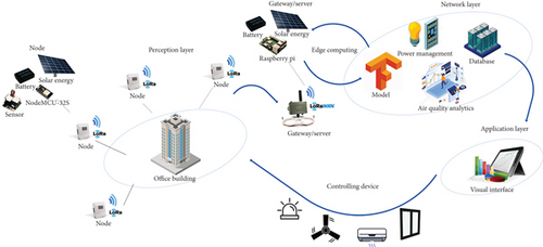
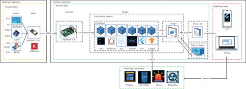
Referring to the conceptual network architecture in Figure 1, the proposed system framework for hardware and software implementations is illustrated in Figure 2. Observe that a microcontroller unit (i.e., the NodeMCU-32S development board [48]) along with sensors, a mobile application, and a web platform are used to design an indoor air quality monitoring system. In the perception layer, the sensor nodes collect and transmit seven types of environmental information (CO2, CO, PM2.5, PM10, VOC, HCHO, CH4) to the NodeMCU-32S. Note that although a certain concentration of SOx and NOx are harmful to the human body, they are not enrolled in the related Act in our country [49]. Therefore, SOx and NOx have not been included in the IoT module. Then, through the network layer, the NodeMCU-32S utilizes LoRa communication technology to send the information to a gateway (e.g., Raspberry Pi) for cloud storage. Subsequently, various services within Docker containers are enabled to analyze the collected environmental information for prediction and regulation. The analytical results are then presented on the mobile application and web platform in the application layer. Finally, the relay activates the pollution control devices and expels the indoor polluted air.
2.2. Hardware Implementation
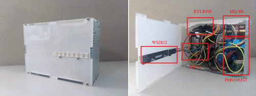
This system utilizes the NodeMCU-32S development board to connect three sensors (MQ-9B [50], PMS5003ST [51], and SGP30 [52]) for measuring nine types of environmental data. Table 3 provides the pinout table for the connections between NodeMCU-32S, sensors, and the LoRa communication module [53], detailing and describing their interconnections.
| Components | NodeMCU-32S | Index |
|---|---|---|
| PMS5003ST | Universal asynchronous receiver/transmitter (UART) | PM2.5, PM10, HCHO |
| MQ-9B | Analog output (AO) | CO, CH4 |
| SGP30 | Interintegrated circuit (I2C) | CO2, VOC |
| RYLR998 LoRa | UART | |
| WS2812 RGB LED | AO |
The enclosure of the air node in this system was designed using computer-aided design (CAD) [54]. To facilitate the assembly of the air node enclosure, each component of the box was designed separately, and the surface was divided into multiple sections based on the connection requirements of different sensors. Finally, these components were integrated together to form a complete enclosure structure, as shown in Figure 3.
2.3. Software Implementation
This subsection presents the implementation of the system software, focusing on sensing calibration with linear regression, classification with the RF model, prediction with the Bi-LSTM model, an application platform with a container, and control mechanisms.
2.3.1. Calibration With Linear Regression
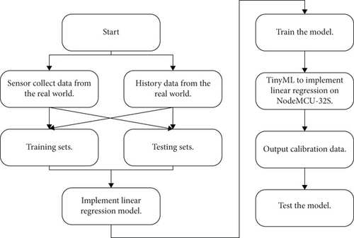
In this context, represents the precise value of PM2.5, b0 represents the estimated intercept of the linear equation, b1 represents the estimated slope of the linear equation, and x represents the sensed value of PM2.5. The system first trains the linear regression model on the PC using accurate PM2.5 data and sensor values. Then, TinyML [55] is used to convert the trained model into a TensorFlow Lite model in resource-limited environments. Finally, the model is deployed onto the development board to enable real-time calibration of sensor data at the edge. Figure 4 illustrates the entire calibration process.
2.3.2. Classification and Control Mechanisms
The indoor air quality control mechanism involves the interactions of five types of gas sensors and hardware devices, including the gases (i.e., CO, CH4, PM2.5, CO2, and VOC) and the management facilities (i.e., windows, air purifiers, exhaust fans, and alarms), as described in Table 4. Accordingly, a set of predefined regulatory guidelines is developed for possible scenarios considering both indoor and outdoor environments. Referring to the categories of gas concentration in Table 1 and given the definition of abnormality as the gas concentrations at moderate and high levels, Table 5 summarizes 10 typical examples of regulatory guidelines, depicting the hardware interactions with respect to gas concentrations and providing the real-time functionality for expelling indoor polluted air. Referring to Regulation 3 in Table 5, when CO, CO2, and PM2.5 are, respectively, at a moderate concentration and CH4 and VOC are, respectively, at a low concentration, the window, air filter, and ventilation fan will be activated. Afterwards, the pollutant control devices will be adaptively activated and deactivated based on the variations in gas concentrations. Given that the window, air filter, and ventilation fan have been activated to improve the air quality and the CO2 is at a moderate concentration, the window and ventilation fan will still be activated. However, the air filter will be deactivated based on the Regulation 6.
| Item | Coping with the situation |
|---|---|
| Alarm | A warning of danger |
| Window | For convection and ventilation |
| Exhaust fan | Work with windows to speed up air circulation |
| Air purifier | Air purification for PM2.5 and VOC |
| No. | Regulation | Logistic with gas concentrations |
|---|---|---|
| 0 | STOP | All gases are normal or CH4 and VOC are at high concentrations (all electrical appliances will be cut off to avoid explosion.) |
| 1 | STAY | 4 gases occur indoors and outdoors with moderate or higher concentrations |
| 2 | A + Wo + N + F | The concentration of 3 gases was abnormal, but the concentration of VOC and CH4 did not reach a high level |
| 3 | A + Wo + N | The concentrations of CO, CO2, and CH4 are abnormal, but CH4 is not at a high concentration |
| 4 | A + Wo + N + F | CO and PM2.5 are abnormal, one of which has a high concentration. |
| 5 | Wo + N + F | CO, CO2, and PM2.5 are at a moderate concentration and CH4 and VOC are at a low concentration |
| 6 | Wo + N | CO2 appears at a moderate concentration |
| 7 | Wo + N + F | PM2.5 is at a moderate concentration |
| 8 | A + Wc + F | Indoor and outdoor PM2.5 is abnormal; outdoor gas is also abnormal and the gas concentrations are high |
| 9 | Wc + F | Indoor and outdoor PM2.5 are abnormal and the gas concentrations are moderate |
- Note: Window: Wo = window open; Wc = window close; air filter: F = air filter open; ventilation fan: N = ventilation fan open; alarm: A = alarm open.
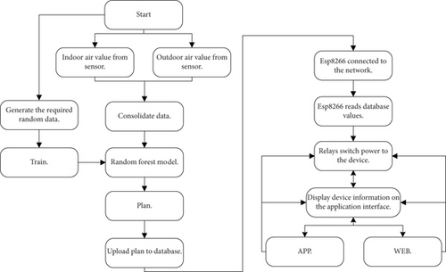
Combining the strengths of the decision tree and bagging algorithms, the RF algorithm is applied for the control model in the proposed system. To fine-tune the algorithm parameters, we employ GridSearchCV to optimize the hyperparameters as detailed in Table 6. Referring to the hardware operations, the regulatory guidelines, and the learning model, Figure 5 illustrates the flow chart of system control procedures.
| Parameter | Range of parameter iteration | Best parameter |
|---|---|---|
| n_estimators | 10~100 (tolerance is 1) | 25 |
| Max_features | 5~50 (tolerance is 1) | 7 |
| Max_depth | 10~80 (tolerance is 1) | 20 |
| Min_samples_split | 10~60 (tolerance is 1) | 30 |
| Min_samples_leaf | 3~20 (tolerance is 1) | 10 |
2.3.3. Prediction of Outdoor Air Quality
Knowing the exact levels of various pollutants in the air is the foundational step in addressing air quality issues. This information is essential for identifying pollution hotspots, understanding temporal trends, and assessing compliance with air quality standards. The source of pollutants is often more localized indoors, with control and management more straightforward. However, since daily activities and the environment both influence the interaction between indoor and outdoor pollutants, the complexity of sources in the outdoor environment may make control and regulation more challenging. Accordingly, we establish a prediction model of outdoor air quality, focusing on PM2.5 local distribution.
To consider the characteristics of PM2.5 data and improve the understanding of temporal relationships and data dependencies in time series data, LSTM-based (i.e., Bi-LSTM, LSTM, LSTM-Attention) and MLP dynamic prediction models are applied. In the time series analysis, dynamic prediction models typically utilize the known past data to forecast the future data points, capturing dynamic features and trends beyond a fixed trend line or mean value. The model is trained using monthly average PM2.5 concentration data from large monitoring stations between 2019 and 2021.
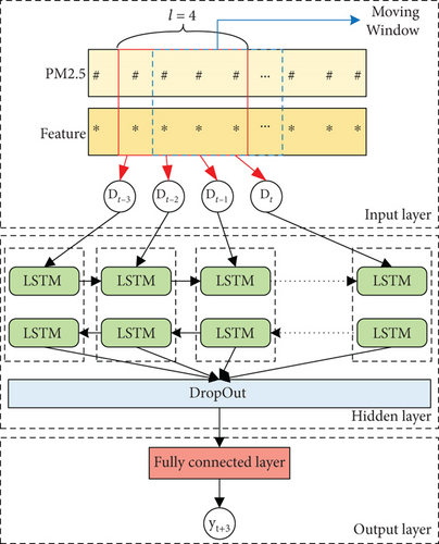
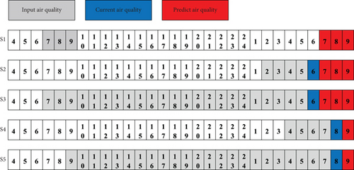
Figure 6 illustrates the range of the moving window in the prediction model, which serves as the input values for the model. Note that Figures 6 and 7, respectively, represent the Bi-LSTM input model and its input formats. In Figure 6, the moving window method allows us to input the latest gas information to achieve dynamic prediction. Furthermore, by using different time periods as the input format for the moving window, as shown in Figure 7, we have validated the impact of varying time period lengths on prediction performance. To evaluate the prediction performance, we process the data with different formats (i.e., S1, S2, S3, S4, and S5) as depicted in Figure 7. Observe that the grey area represents the historical input data, the blue area represents the current input data, and the red area represents the predicted data. In the S1 format, we include the data from the same time period of the previous day as part of the input. The S2 to S5 formats are applied to investigate the impact of data with different time intervals on the prediction performance, such as inputting data from the past 5 h or 24 h and predicting the 1-h or 3-h air quality. Please refer to Figure 7 for more details.
2.3.4. Land Use Regression (LUR) Model
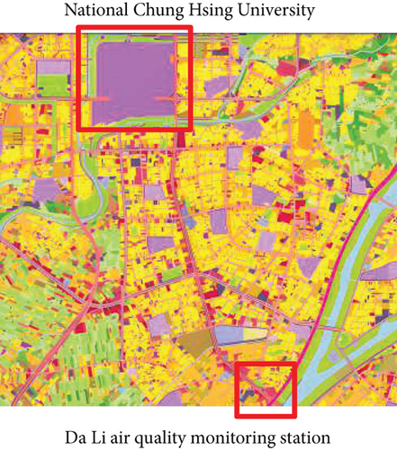
Since outdoor pollution can be influenced by land-use decisions [56], the density of traffic, and industrial activities, this study combines geographic information systems (GISs) and air quality monitoring data from stations to establish a LUR model for describing the emission characteristics. The LUR model utilizes geographic information, land use data, and other relevant features to predict the distribution of pollutants. In previous practices, it is common to include all parameters in the model for training, without undergoing feature selection (e.g., the Bi-LSTM model as shown in Figure 6). To further depict the long-term spatiotemporal distribution of PM2.5, here, the LUR model is used for feature selection with the aim of gaining a deeper understanding of the distribution and trends of pollutants. The Environmental Protection Administration has established a total of 76 air quality monitoring stations across the island, including three stations on outlying islands. The selection of these stations is based on factors such as geographical location, meteorological conditions, population distribution, pollution source distribution, and monitoring needs in each region. For this study, the monitoring station of the Da-Li district, which is near the monitoring site of the outdoor air at National Chung Hsing University (NCHU), is chosen to establish the LUR model. Monthly average concentrations of air pollutants (e.g., PM2.5, NO2, O3, and SO2) from 2016 to 2021 are analyzed, along with meteorological information such as temperature and relative humidity.
The land use survey records the land use status using colors and annotations, as shown in Table 7 and Figure 8. The survey focuses on utilizing high-resolution remote sensing imagery to understand the current state of land use. It combines geospatial data such as cadastral maps and topographic maps to enhance the national land information system and the basic land database, meeting the needs of various authorities for land management.
| Database | Data | Data relevance | Data description | |
|---|---|---|---|---|
| Air Quality Information from Environmental Protection Administration (EPA) | PM10 | + | ug/m3 | |
| PM2.5 | + | ug/m3 | ||
| NO/NO2 | + | ppb | ||
| SO2 | + | ppb | ||
| O3 | + | ppb | ||
| CH4 | + | ppb | ||
| CO | + | ppb | ||
| Temperature | + | C | ||
| Relative humidity | − | % | ||
| Precipitation | − | % | ||
| Wind speed | + | m/s | ||
| Wind direction | + | 360° | ||
| Land Use Survey | Land use for building | Yellow | + | The area of the measuring station within a radius of 500–6000 m (m2) |
| Land use for agricultural | Green | + | ||
| Land use for water | Blue | − | ||
| Land use for recreation | Orange | − | ||
| Land use for forest | Dark green | + | ||
| Land use for transportation | Red | + | ||
| Empty land | Black | − | ||
| Land use for mining | Brown | + | ||
| Land use for public | Dark yellow | − | ||
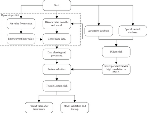
Integrating the prediction and LSU models, Figure 9 depicts the prediction flowchart, in which the system utilizes a BiLSTM model for the dynamic prediction of given data. Prior to making predictions, the system also undergoes a feature selection step to eliminate features that lack predictive power or are redundant, thereby enhancing the effectiveness and efficiency of the prediction model. This approach enables the establishment of an accurate and efficient prediction model to meet various data prediction requirements.
2.4. Application Platform
The application web page of this system is developed using the LAMP [57] architecture, integrating Linux, Apache, MySQL, and PHP. To manage and run applications more flexible, the Docker platform with Raspberry Pi is deployed in this work. The design concept of this system is to launch individual containers for each function, such as LoRa transmission, prediction, control, database, and web backend, as illustrated in Figure 10. By enabling communication between different containers, the desired services can be achieved. Building with separate containers allows for easier isolation, deployment, and scalability of distributed applications and microservices. Additionally, it facilitates deployment across multiple operating systems and hardware platforms. Figure 10 presents the basic configuration for Docker compose and system architecture of containerized application for air quality control.

3. Results and Discussion
This section investigates the performance of the proposed system architecture as follows: (1) evaluate the effectiveness of the prediction model; (2) explore the classification accuracy of the regulation algorithm; (3) conduct tests on the calibration algorithm running on an embedded development board; (4) present and analyze the simulation results of indoor airflow; (5) detail the system configuration of the Docker environment; and (6) showcase the presentation of the application’s mobile app and web interface.
3.1. Prediction Effectiveness
3.1.1. Performance Without Feature Selection
Table 8 summarizes three performance metrics used for data analysis and performance evaluation (i.e., MAE, RMSE, and mean absolute percentage error (MAPE), where MAPE is a measure of prediction accuracy of a forecasting method in statistics, considering estimated measurement values and reference measurement data). Note that reference measurement data (actual values), the mean of reference measurement data, and estimated data are represented by yi, , and , respectively. The symbol i denotes the index of the data, while n represents the total number of data points. Tables 9 and 10 present analyses of the performance of a prediction model in terms of RMSE and MAE, respectively. Based on the tables above, it can be observed that the Bi-LSTM model outperforms other models in terms of both RMSE and MAE performance metrics. Referring to the input format in Figure 7, predicting the specific time interval using historical data with the same time period (i.e., data with the S1 format) yields better results compared to those using shorter (5 h) or longer (24 h) time periods for prediction.
| Performance metrics | Function |
|---|---|
| Root mean squared error (RMSE) | |
| Mean absolute error (MAE) | |
| Mean absolute percentage error (MAPE) |
| RMSE metric | |||||
|---|---|---|---|---|---|
| Model | S1 | S2 | S3 | S4 | S5 |
| Bi-LSTM | 8.43 | 9.001 | 9.228 | 9.34 | 10.05 |
| LSTM | 9.587 | 10.43 | 9.377 | 9.94 | 10.22 |
| LSTM-Attention | 12.286 | 12.369 | 12.827 | 13.1 | 13.493 |
| MLP | 12.62 | 12.45 | 13.02 | 13.449 | 14.692 |
- Note: The entries in bold represent the best prediction performance among the prediction models, with respect to five different data formats.
| MAE metric | |||||
|---|---|---|---|---|---|
| Model | S1 | S2 | S3 | S4 | S5 |
| Bi-LSTM | 6.63 | 7.003 | 6.531 | 6.678 | 7.565 |
| LSTM | 6.956 | 7.428 | 7.43 | 7.538 | 7.95 |
| LSTM-Attention | 7.256 | 8.059 | 9.47 | 8.578 | 10.625 |
| MLP | 8.64 | 10.614 | 10.4 | 12.76 | 12.52 |
- Note: The entries in bold represent the best prediction performance among the prediction models, with respect to five different data formats.
3.1.2. Performance With Feature Selection
This study utilized historical data from the air quality monitoring station of Da-Li District in the central air quality region in Taichung from 2016 to 2021, as well as the land use status survey map for the year 2020, as shown in Figure 8. Eighteen variables were considered, including air pollutants (NO2, SO2, and O3), meteorological factors (temperature and relative humidity), and variables related to land use, such as agricultural land area and traffic area. Figures 11 and 12, respectively, show the correlation between environmental factors and PM2.5 and the correlation between geographic factors and PM2.5.
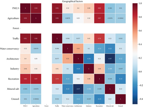
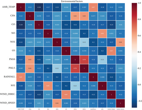
The overall results of the LUR model developed in this study have been summarized in Table 11 with the 10 selected environmental factors (i.e., ambient temperature, CH4, CO, NO2, O3, PM10, and wind speed) and the geographic factors (i.e., agriculture, recreation, and traffic zones). Referring to Tables 12 and 13 with feature selection, it can be observed that compared with the performance of Tables 9 and 10 without feature selection, the performance improves with an increase in accuracy and a smaller increase in loss. Without loss of generality, the data analysis shows that using the S1 input format (i.e., similar input data during the same time interval on different days) leads to optimal prediction results. This phenomenon is likely attributed to people’s daily routines, especially during commuting hours or dinner times, where factors such as increased traffic flow and cooking fumes from main dishes may indirectly impact the readings at the monitoring station. It is noteworthy that we further refined our analysis by filtering out variables that do not correlate with PM2.5 through feature selection, thereby enhancing the accuracy of S1 predictions.
| LUR model | ||||
|---|---|---|---|---|
| Parameter | Coefficient | Standard error | Test statistic | p value |
| AMB_TEMP | 0.097 | 1.6377 | 9.0435 | < 0.01 |
| CH4 | 0.64 | 0.0531 | 21.9134 | < 0.01 |
| NO2 | 0.13 | 0.0112 | 9.6672 | < 0.01 |
| PM10 | 0.79 | 0.0084 | 79.333 | < 0.01 |
| WIND_SPEED | 0.023 | 0.0548 | 2.0626 | < 0.01 |
| Agricultural | 0.928 | 0.0234 | 4.7463 | < 0.01 |
| Transportation | 0.9138 | 0.0098 | 5.6753 | < 0.01 |
| Recreation | 0.832 | 0.1009 | 4.4567 | < 0.01 |
| RMSE metric | |||||
|---|---|---|---|---|---|
| Model | S1 | S2 | S3 | S4 | S5 |
| Bi-LSTM | 8.185 | 8.564 | 9.1 | 9.309 | 9.332 |
| LSTM | 8.249 | 9.135 | 9.268 | 9.887 | 10.192 |
| LSTM-Attention | 8.229 | 8.827 | 9.853 | 10.052 | 11.424 |
| MLP | 9.806 | 11.174 | 12.252 | 13.43 | 12.456 |
- Note: The entries in bold represent the best prediction performance among the prediction models, with respect to five different data formats.
| MAE metric | |||||
|---|---|---|---|---|---|
| Model | S1 | S2 | S3 | S4 | S5 |
| Bi-LSTM | 5.74 | 6.295 | 6.371 | 6.547 | 6.742 |
| LSTM | 6.819 | 7.416 | 7.468 | 7.415 | 7.492 |
| LSTM-Attention | 7.121 | 7.336 | 7.528 | 7.599 | 7.698 |
| MLP | 7.385 | 8.465 | 8.523 | 8.734 | 8.525 |
- Note: The entries in bold represent the best prediction performance among the prediction models, with respect to five different data formats.
3.1.3. Comparative Analysis
This work tests the prediction accuracy of MLP and RNN models. MLP is commonly used for simple arithmetic and linear regression problems, but it performs poorly when handling sequential data and requires a large number of parameters. In contrast, RNN excels at processing sequential data, as it can effectively capture dependencies in historical data, making it beneficial for prediction tasks. Among the three RNN models (i.e., LSTM, Bi-LSTM, and LSTM-Attention) tested in this study, LSTM addresses the vanishing gradient problem in traditional RNNs when dealing with long sequences and can better capture temporal correlations. Bi-LSTM further enhances the model by incorporating contextual information from both directions, overcoming the limitation of unidirectional LSTM. LSTM-Attention allows the model to focus on key information in long sequences, thereby improving prediction accuracy. The experimental results show that the Bi-LSTM achieves the best predictive performance among the above three RNN models with a MAE of 5.74 and a MAPE of 15.4%.
In [35], Bi-LSTM and wavelet conversion techniques were used to predict air quality. The model first uses wavelet transformation to decompose the air quality data into components of different frequencies, and then extracts valuable feature information for prediction, and achieves a MAE of 6.72 and a MAPE of 16.39%. In [36], CNN was applied to time series data forecasting and combined with the LSTM model to predict the value of the next 24 h. Eventually, the model achieved an average absolute error of 6.52. In [38], the air quality index using time series and deep learning methods is examined. A CNN-LSTM model is proposed to improve the air quality prediction accuracy, where CNN’s efficient feature extraction function is used to extract data features, achieving a MAE of 21.14 and a MAPE of 32%.
Compared with the methods in [35, 36, 38], using wavelet-based Bi-LSTM, CONV-LSTM, and CNN-LSTM as prediction models, the main difference between these three methods and the proposed model lies in the feature extraction method, which decomposes the features into spatial and temporal components. In terms of spatial feature extraction, we apply a land regression model to screen out gases that have been associated with PM2.5 through geographical environment factors and remove irrelevant factors. On the other hand, temporal feature extraction focuses on the feature relationships at different time scales and uses data from the same interval as input to improve the accuracy of prediction in the same time interval. Accordingly, the current prediction results are corrected based on the real-time dynamic air quality data. Table 14 summarizes the MAE and MAPE error performances of the models in [35, 36] and [38], the proposed model without feature extraction, and the proposed model with feature extraction, which implies that comparing to the above static models in [35, 36] and [38], the proposed Bi-LSTM model with feature selection delivers higher PM2.5 prediction accuracy by about 14.58%, 11.96%, and 72.85% in terms of the MAE error performance.
3.2. Classification
In this experiment, we applied three different models, namely, RF, decision tree, and bagging, fed with the 12,525 pieces of randomly generated data according to the regulation guidelines mentioned in Table 6 for model learning. Table 15 displays the performance comparison of the three models with 1,001,000 data points, providing the information of the confusion matrix and classification report. It is observed that RF achieves the highest accuracy and F1 score. Referring to the regulation guidelines in Table 6 and the classification results in Table 15, the condition for Regulation 8 is that only PM2.5 exceeds the standard value, while the other gases remain within acceptable levels. Regulations 0, 1, and 2, on the other hand, encompass three or more gases with general regulation guidelines, while the remaining labels have specific standards set for individual gases. Thus, there might be a high degree of overlap between Regulation 8 and Regulations 0, 1, and 2, which may impact the classification results.
| Random Forest | |
| Confusion matrix | Classification report |
 |
 |
| Decision tree | |
 |
 |
| Bagging | |
 |
 |
3.3. Indoor Flow Field Analysis
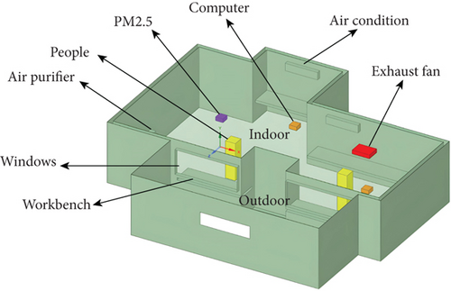
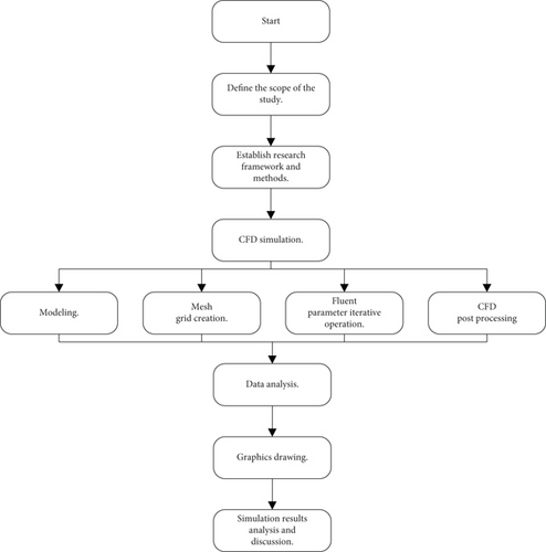
This work employs numerical simulation analysis to model a system with automatic control of indoor pollution control devices. The research utilizes a CFD-based numerical simulation software, CFD-FLUENT [58], to simulate, analyze, and compare the airflow within indoor spaces. The objective of the study is to comprehensively investigate whether the indoor concentration of harmful gases could be effectively and rapidly reduced after activating specific pollution control devices. In the simulation, Room 731 in the Applied Science and Technology Building at NCHU is used as the basis for a 3D model created to scale. The indoor and outdoor spaces, air purifiers, windows, exhaust fan, air conditioning, and other relevant parameters are imported into the FLUENT software, as shown in Figure 13 and Table 16. Note that the floor area is about 85 m² and the ceiling height is about 2.3 m. The simulation method used in this study is based on the research tool Ansys Fluent 2021. The main operational workflow can be divided into three parts: preprocessing, parameter configuration, and postprocessing. Users can visualize the calculation results through a graphical interface. Please refer to Figure 14 for the CFD solution process.
| Setting | Condition | ||
|---|---|---|---|
| Initial conditions | The initial indoor temperature is 24°C, and the grid is 310,000. | ||
| Boundary conditions | Equipment | Speed | Flow direction |
| Exhaust fan | 2 m/s. | In | |
| Windows | 0.2 m/s. | Out | |
| Air conditioner | 0.39 m/s. | Out | |
| Air purifier | 0.39 m/s. | Out | |
| Equipment | Diffuse gas | Flow rate | |
| Door | PM2.5 | 0.1 m/s | |
| People | CO2, CO | Heat 43w/m2, 0.1 m/s | |
| Workbench | VOC, CH4, CO2, CO | 0.1 m/s | |
| Computer | CO2, CO | Heat 43w/m2, 0.1 m/s | |
| Outdoor | ALL | ||
- •
Scenario 1:
- 1.
Air quality: Indoor CO, CO2, and PM2.5 have a moderate concentration, while CH4 and VOC have a low concentration.
- 2.
Sewage equipment: sprinkler/open window/air purifier/exhaust fan.
- •
Scenario 2:
- 1.
Air quality: Indoor PM2.5 has a moderate concentration, while outdoor gases (CO2 and CO) are abnormal and reach dangerous concentration levels.
- 2.
Sewage equipment: alarm/close window/air purifier.
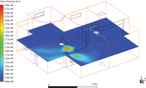
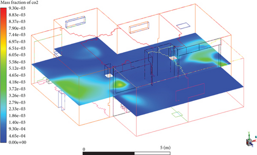
After analyzing the indoor and outdoor gas concentrations in the two different scenarios mentioned above, Figures 15, 16, 17, and 18 show that the proposed system effectively eliminates the sources of pollution. In Figures 15 and 16 of Scenario 1, we observe that higher concentrations of CO, CO2, and PM2.5 in the area, where the distribution of the above individual gas is in the laboratory, are depicted in Figures 15a, 15b, and 15c, respectively. Figure 15c also illustrates the infiltration of outdoor PM2.5 into the indoor environment. Moreover, Figure 15d,e reveals elevated concentrations of CH4 and VOC in the area around desks, chairs, and computers. These five gases may disperse towards pollution control devices, air purifiers, exhaust fans, and windows to be eliminated to safe concentrations. With Regulation 5 presented in Table 6, it is noteworthy that when harmful indoor gases accumulate to a certain level, the activation of pollution control devices takes only 1 min to restore indoor air quality to normal levels, as depicted in Figure 16, which shows a descending trend in air concentrations of CO, CO2, PM2.5, and CH4. This underscores the efficiency and real-time response of the equipment in Regulation 5, contributing to the maintenance of indoor air quality.
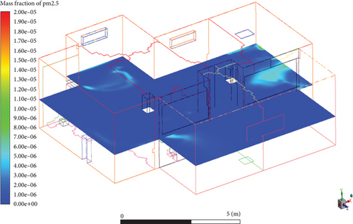
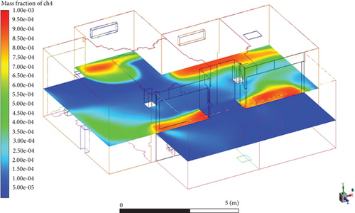
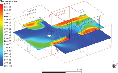
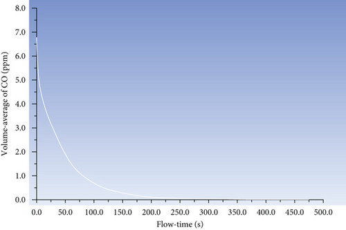
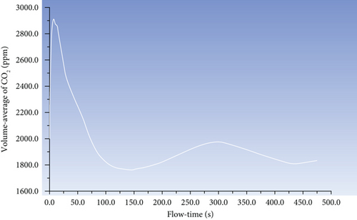
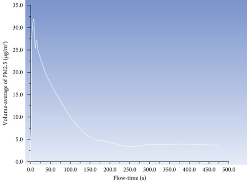
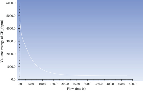

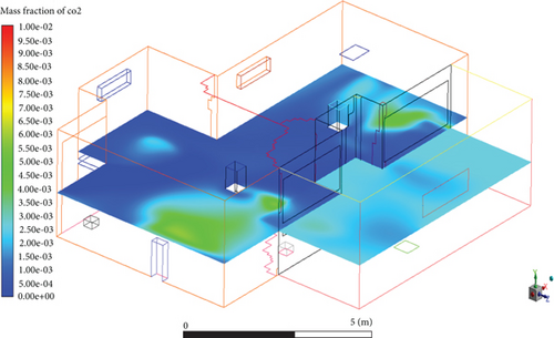
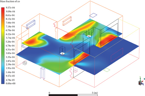
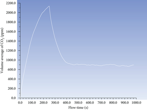
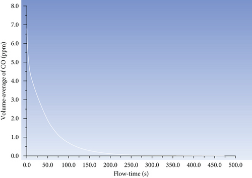
In Figures 17 and 18 of Scenario 2, we simulated a scenario with closed windows and the corresponding airflow patterns and distributions. Similar to the results in Figures 15 and 16. Figures 17 and 18 show that Regulation 2 not only eliminates indoor pollutants but also effectively prevents outdoor polluted air from entering the building. By utilizing exhaust ventilation and air purifiers, we are able to expel the indoor polluted air to the outside. Simultaneously, the action of closing doors and windows effectively prevents outdoor polluted air from entering indoors. Most importantly, once the indoor gas concentration reaches a normal level, the system immediately shuts off the pollution control devices, thereby reducing the power consumption.
3.4. Application Platform
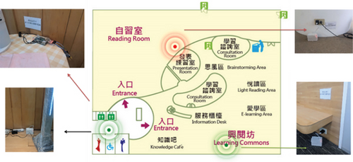
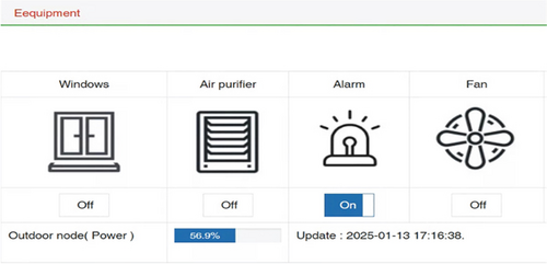
This section showcases the features of the web interface, where these functionalities are directly applied to the experimental results. To assess the feasibility of the proposed system, we consider the reading area located on the first basement (B1) floor of the NCHU library as the validation site. The web interface of the proposed system consists of the live air quality map (Figure 19), the device control information page (Figure 20), and the prediction page (Figure 21). The live air quality map and field verification page displays the concentration of PM2.5 based on the positions of nodes in different areas with red dots indicating abnormal levels and green dots indicating normal levels. The device control information page provides users with insights into the operational status of the devices and allows control of the environment’s equipment through the web interface, enabling bidirectional control. The prediction information page enables users to view air quality information for the next 3 h, presented in a line chart with the green line. Note that the above functionalities and page designs will be directly applied to the experimental results.

4. Conclusions
This work proposes an IoT-based air quality system that improves upon monitoring and pollution control performance. Compared with existing traditional air pollution monitoring systems in the market, our system exhibits high scalability and compatibility by introducing automated node devices and systems, reducing the need for human resources. Using the Ansys CFD airflow simulation software, we confirm that the proposed method effectively and rapidly removes pollutants, accomplishing our intended goals. Moreover, with Docker containers, users can easily manage the development environment. In addition to saving implementation costs, the system enables seamless adjustments in the future for site relocation or expansion. Besides using Docker for rapid deployment of monitoring and control systems, we have also designed two application platforms that enable continuous 24 h monitoring, which provide graphical interfaces that allow users to visualize environmental changes and adjust the operation or maintenance schedules of equipment in the field. This helps reduce the cost of electricity consumption for equipment within the field.
In the future, we aim to expand the application scope of the air management system, not limited to libraries and office buildings, but also extensively applied in factories and households, among other diverse settings, which will enable us to comprehensively understand and manage indoor air pollution in various environments. Moreover, higher concentrations of NOx, SOx, etc. are also harmful to the human body. However, they are not enrolled in the related act in our country [59]. As a result, they were not included in the IoT module and become the limitation of this work. This will be addressed in the future work.
Nomenclature
-
- AE
-
- autoencoder
-
- ANN
-
- artificial neural networks
-
- ARIMA
-
- autoregressive integrated moving average
-
- Bi-LSTM
-
- bidirectional long short-term memory
-
- CFD
-
- computational fluid dynamics
-
- CH4
-
- methane
-
- CO
-
- carbon monoxide
-
- CO2
-
- carbon dioxide
-
- CONV-LSTM
-
- convolutional long short-term memory
-
- CNN
-
- convolutional neural networks
-
- EMD
-
- empirical mode decomposition
-
- EPA
-
- environmental protection administration
-
- GA
-
- genetic algorithm
-
- GIS
-
- geographic information systems
-
- GRU
-
- gated recurrent unit
-
- HCHO
-
- formaldehyde
-
- IoT
-
- Internet of Things
-
- LSTM
-
- long short-term memory
-
- LUR
-
- land use regression
-
- LUR-Dynamic Bi-LSTM
-
- land use regression–based bidirectional long short-term memory
-
- MAE
-
- mean absolute error
-
- MAPE
-
- mean absolute percentage error
-
- MLP
-
- multilayer perceptron
-
- NCHU
-
- National Chung Hsing University
-
- NH3
-
- ammonia
-
- NO2
-
- nitrogen dioxide
-
- O3
-
- ozone
-
- PM
-
- particulate matter
-
- RBF
-
- radial basis function
-
- ResNET
-
- residual neural networks
-
- RF
-
- random forest
-
- RMSE
-
- root mean square error
-
- RNN
-
- recurrent neural network
-
- SVD
-
- singular value decomposition
-
- SVR
-
- support vector regressor
-
- VOC
-
- volatile organic compounds
-
- WRF
-
- weather research and forecasting
-
- XGBoost
-
- extreme gradient boosting
Disclosure
The funders had no role in the design of the study; in the collection, analyses, or interpretation of data; in the writing of the manuscript; or in the decision to publish the results.
Conflicts of Interest
The authors declare no conflicts of interest.
Funding
This work was supported by the National Science and Technology Council, Taiwan, under Grant 113-2221-E-005-014, and the Smart Sustainable New Agriculture Research Center (SMARTer), National Science and Technology Council, Taiwan, under Grant 113-2634-F-005-002.
Open Research
Data Availability Statement
For this study, the monitoring station of the Da-Li district, which is near the monitoring site of the outdoor air at National Chung Hsing University (NCHU), is chosen to establish the LUR model. Monthly average concentrations of air pollutants (e.g., PM2.5, NO2, O3, and SO2) from 2016 to 2021 are analyzed, along with meteorological information such as temperature and relative humidity (https://data.moenv.gov.tw/dataset/detail/AQX_P_218).


