The vibration signal of rolling beating is nonlinear and nonstationary, which makes feature extraction difficult for fault diagnosis. To improve the efficiency of feature extraction and fault diagnosis, a hybrid model based on optimized variational mode decomposition (VMD), fuzzy dispersion entropy (FDE), and a support vector machine (SVM) is proposed. Firstly, a parameter optimization method using the sparrow search algorithm (SSA) was applied to VMD to improve the decomposition ability. Subsequently, a feature vector based on the FDE was proposed as a fault-diagnosis feature. Finally, SVM was applied with the proposed feature vector for the fault diagnosis of rolling bearings. The simulation and experimental study results indicate that the proposed method can obtain useful features for fault diagnosis, particularly in short-length samples and noise conditions. The proposed method performed well in the fault diagnosis for different fault types and degrees of rolling bearings.

1. Introduction

Rolling bearings play an important role in a wide range of applications, such as vehicles, pumps, and motors. They often operate under variable working conditions with long-term working hours, which may cause rolling bearing failures to occur [1]. In general, rolling bearing failures can cause a larger range of failures, which can lead to serious accidents. Therefore, it is necessary to conduct fault detection and diagnosis for rolling bearings to ensure their safety and stability.

The fault diagnosis of rolling bearings primarily involves vibration signals [2], sound signals [3], and infrared thermal imaging [4]. Because the vibration signal includes rich information and is convenient to collect, it is most widely used for fault diagnosis. The features of a vibration signal usually change when the state is unstable or a fault occurs [5]. Thus, the feature extraction of vibration signals is the core issue of fault diagnosis in rolling bearings. The fault diagnosis features of vibration signals in existing research can be divided into two main categories: time and frequency features and entropy features [6, 7].

As time and frequency features can reflect the vibration signal directly and have a significant physical description, they have received considerable attention. Many time and frequency signal processing methods have been proposed, such as the fast Fourier transform (FFT), short-time Fourier transform (STFT), wavelet transform (WT), and Wigner–Ville distribution (WVD) [8–11]. However, these methods have some limitations in terms of processing nonlinear and nonstationary signals; for example, FFT cannot directly reflect the characteristics of data frequency variation over time, and the selection of the wavelet basis and filtering function has a significant influence on the WT [12]. Empirical mode decomposition (EMD) can decompose nonlinear and nonstationary signals into several intrinsic mode functions (IMFs), which are suitable for the signal processing of rolling bearings [13]. Ensemble empirical mode decomposition (EEMD) increases the randomness of the signal by adding noise to the original signal, resulting in a stronger decomposition ability [14]. EEMD solves the problem of mode mixing in EMD. However, both EMD and EEMD are sensitive to noise, which can result in inaccurate IMF components. Variational mode decomposition (VMD) is a signal processing method evolving from EMD that can avoid endpoint effects and fake component problems, and it has strong antinoise capability [15].

Entropy reflects the complexity of vibration signals [16]. The entropy value of the vibration signal changes when the running state of the rolling bearing changes [17]. Many researchers have applied entropy as a feature in the fault diagnosis of rolling bearings. The approximate entropy (AE) can reflect the similarity degree of patterns in a time series and can be applied to the classification of fault characteristics; its effectiveness is limited to extremely short sequences or extremely noisy data [18]. However, the computational complexity of AE is high, and the calculation results are influenced by the parameter selection. Sample entropy (SE) is similar to AE in that it reflects the probability of new patterns appearing in a time series and measures their complexity [19]. The advantage of the SE is that the calculation result is independent of the data length. Similar to AE, the selection of calculation parameters also influences the entropy value. Permutation entropy (PE) can determine the complexity and orderliness of a system by calculating the probability of different arrangement patterns appearing [20]. However, PE is sensitive to noise and has a high computational cost. Dispersion entropy (DE) overcomes some disadvantages of other entropies [21]. It has a fast calculation speed and is less affected by mutation signals, which has made it widely used in the fault diagnosis of rolling bearings in recent years [22–24]. Fuzzy dispersion entropy (FDE) is a new entropy concept proposed in 2022 by Mostafa et al. It is less sensitive to signal data length and has better noise resistance [25, 26].

In this study, a novel hybrid fault diagnosis model is proposed. Parameter optimization of VMD and feature extraction based on FDE are proposed to obtain fault diagnosis features. A support vector machine (SVM) is applied for fault classification.

The remainder of this paper is organized as follows. The theoretical background and the proposed methods are introduced in Section 2. In Section 3, a simulation is presented to analyze the ability of different signal processing methods in a rotating system. In Section 4, the experiments conducted to verify the advantages of the proposed method are presented. Finally, conclusions are presented in Section 5.

2. Theoretical Background and Methods

2.1. FDE

DE is an index that reflects the degree of signal irregularity. As DE can effectively reflect the changes in signal amplitude and frequency at the same time and has less calculation time, it has been widely used in fault diagnosis by many researchers. However, in the DE calculation process, the round function makes the DE value sensitive to the data length, noise, and parameter selection [25]. To solve these problems, FDE is proposed. The FDE value of a time series x = [x₁, x₂, ⋯, x_N] with a data length N is calculated as follows:

Step 1: The element value of the original time series was normalized between 0 and 1 using the normal cumulative distribution function.

()

where y_i(i = 1, 2, ⋯, N) is the element value of the time series after normalization and σ² and μ are the variance and mean values of time series x, respectively.

Step 2: The elements of y are mapped to time series z^c according to Equation (2).

()

where c is the number of the classes.

Step 3: In DE, z^c is classified according to the proximity of integer classes, which may lead to ambiguity. The fuzzy membership function

is applied to represent the degree of membership between each

to the kth class (k = 1, ⋯, c). The fuzzy function refers to the result in Reference [25]. The fuzzy functions can be expressed as follows:

()

Then, every is assigned to one or two classes by the fuzzy membership function.

Step 4: The embedding vector is formed as follows:

()

where m is the embedding dimension and d represents the time delay.

Step 5: The dispersion pattern can be expressed as follows:

()

The number of dispersion pattern is c^m.

Each embedding vector

is mapped to the dispersion pattern according to its degree of membership. The degrees of membership can be calculated based on the t-norm, and the algebraic product operator is used to represent the t-norm as follows:

()

where

is the degree of membership of

mapping to dispersion pattern

Step 7: The probability of each dispersion pattern is calculated as follows:

()

Step 8: The FDE value of time series x with embedding dimension m, number of classes c, and time delay d can be expressed as follows:

()

2.2. VMD

VMD is an effective signal-processing method for nonlinear and nonstationary signals. The original signal can be decomposed into a series of IMFs with limited frequency bandwidth as described in Equation (9) [15].

()

where f(t) represents the time-domain original signal, K is the number of IMFs, u_k(t) is the kth IMF of the original signal, and ω_k is the center frequency of u_k.

Because the minimization problem in Equation (9) cannot be solved directly, an extended Lagrangian function was applied:

()

where α is the penalty factor and η represents the Lagrange multiplier.

The minimization problem is then transformed into a saddle point problem, which can be solved by an iterative search as follows:

()

where u_k(ω), f_k(ω), and η_k(ω) represent frequency domain of u_k(t), f_k(t), and η_k(t), respectively. τ is the updating step.

2.3. The Proposed Method

In this paper, a VMD with parameter optimization is proposed to obtain multiple modals of different frequency centers and decrease the influence of noise simultaneously. A feature vector, which is formed by FDE, was also proposed for the SVM for fault diagnosis. The flowchart of the proposed method is shown in Figure 1. The detailed process and the highlights of the proposed method are introduced in Sections 2.3.1 and 2.3.2.

Details are in the caption following the image — **Figure 1**
Open in figure viewer PowerPoint

The flowchart of the proposed fault diagnosis method.

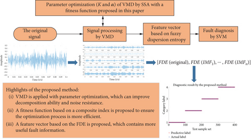
2.3.1. Parameter Optimization of VMD

VMD exhibits outstanding performance in nonstationary signal processing. However, the number of extracted modal K and modal frequency bandwidth control parameters α must be assigned primarily. If K is set too large or too small, it will cause overdecomposition or a lack of decomposition. Parameter α will cause missing frequency band information if α is set too large. This results in increased frequency band information redundancy and computational complexity if α is set too small.

To obtain suitable parameters for VMD, reasonable evaluation indicators must be proposed. In this study, two factors were considered as the optimal parameters for VMD.

Firstly, the FDE represents the complexity and fluctuation of the time-domain signal. The IMFs acquired by suitable VMD parameters are more regular and have less noise, and the FDE of the IMFs is smaller. Therefore, the FDE can be utilized as an indicator to evaluate the performance of VMD processing.

Secondly, mutual information (MI) is used to evaluate the richness of the IMF features. If the IMF contains more feature information, the MI value increases. MI can be described as follows:

()

where mi represents the value of MI in a normalized format, MI is the mutual information, and X and Y represent different events. H(Y) is the entropy of Y and H(Y|X) is the conditional entropy of Y.

IMFs with higher MI values contain more feature information. Therefore, a fitness function based on a composite index for parameter optimization of the VMD is proposed as follows:

()

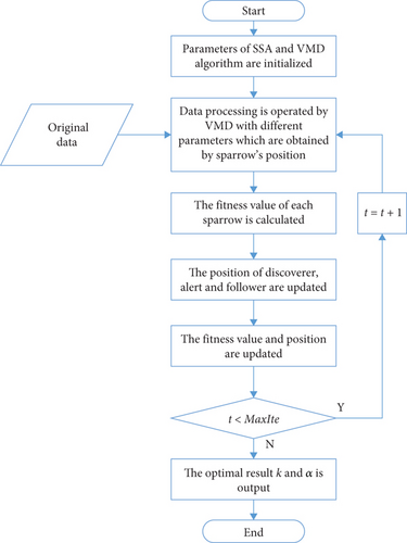
In this study, the sparrow search algorithm (SSA) was utilized to obtain the optimized parameters of the VMD using the fitness function proposed above. The SSA is a swarm intelligence optimization algorithm known for its fast calculation speed and good robustness [27]. The steps of the parameter optimization of VMD by SSA are as follows:

Step 1: initialize the algorithm parameters. The parameters include the number of sparrows nPop, the maximum number of iterations MaxIte, safety value ST, and dimensions and boundaries of the optimization problems. The positions of the sparrows were initialized.

Step 2: obtain the values of K and α for each sparrow according to the position. The original data were processed using VMD with different K and α values. And the fitness is calculated with the IMFs according to Equation (15). The fitness is then sorted to find the individual with the current best fitness and its current best position.

Step 3: The sparrow position is updated using different rules. The positions of the discoverers with better fitness were updated using Equation (16) as follows:

()

where

represents the position of the ith sparrow in the jth dimension of the tth iteration, η ∈ (0, 1] is a random number, R2 ∈ (0, 1] is an alert value, ST ∈ [0.5, 1], Q is a random number with a normal distribution, and L represents a matrix with 1 × d with all one elements.

The position of followers is updated as follows:

()

where X_worst is the worst position of the current global, X_p is the best position of the current global, and A is a matrix satisfying

The position of the alert that is aware of danger is updated as follows:

()

where

represents the best position of the tth iteration, β is a step size control parameter with normal distribution, K is a random number, f_i represents the fitness of the ith sparrow, f_g is the global best fitness, f_w is the global worst fitness, and ε is a small constant.

Step 4: The fitness of each sparrow was compared before and after the position update, and a better position was selected. Then, the position of the sparrow with the best fitness is updated.

Step 5: The position of the sparrow with the best fitness is output until the maximum number of iterations is reached. Otherwise, Steps 3 and 4 were repeated.

The flowchart of the parameter optimization of the VMD by SSA is shown in Figure 2.

2.3.2. Feature Extraction Based on FDE

The vibration signal of a rolling bearing is highly complex in different running states, which makes it difficult to reflect all the characteristics of a fault using a single FDE. As the vibration signal can be decomposed into different frequency bands, FDE can also be acquired in different frequency bands, which will benefit the acquisition of more useful fault diagnosis features. In this study, a vibration signal feature extraction method based on VMD and FDE is proposed for the fault diagnosis of rolling bearings. The steps of the method are as follows:

I.
The FDE of the original vibration signal FDE(original) was calculated to reflect the characteristics of the original signal.
II.
The vibration datasets u₁(t), u₂(t), ⋯, u_m(t) in different running states are decomposed by VMD. Because different datasets have different optimal parameters K_u1, K_u2, ⋯, K_um, the number of IMFs of different datasets is not consistent. To ensure consistent dimensionality of the feature vectors, the former K = min{K_u1, K_u2, ⋯, K_um} modal is selected to form the fault feature.
III.
The FDE of each IMF of the vibration signal was calculated. The feature vector based on the FDE can be described as follows:

()

3. Simulation Analysis

Because of the nonlinear and nonstationary characteristics of the rolling bearing signals, it is difficult to extract the fault features using a normal signal processing method.

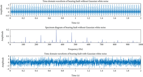
In this section, a rolling bearing fault model is used to simulate the fault signal of the inner race fault. The WT, STFT, EMD, and VMD are applied to test the ability of the time-frequency analysis, which will also verify the signal processing method proposed in this paper.

The inner race early failure model of the rolling bearing is described as follows:

()

where y(t) is the fault vibration signal with Gaussian white noise, s(t) is the periodic impact component, and n(t) is Gaussian white noise. Signal-to-noise ratio (SNR) is set as −13 dB. A₀ is the amplitude, which is set as 0.5; f_r is the rotation frequency of the bearing, which is set as 30 Hz; C is the attenuation coefficient, which is set as 500; and f_n is the resonance frequency, which is set as 400 Hz. The characteristic frequency of the inner race fault was set to f_i = 1/T = 120 Hz, the sampling frequency was 2000 Hz, and the sampling time was 2 s.

The simulated vibration signals in the time domain and frequency domain are shown in Figure 3.

The WT, STFT, EMD, and VMD are applied to obtain the time-frequency spectrogram, where EMD and VMD are combined with Hilbert-Huang transform (HHT) to obtain the time-frequency spectrogram. The results are shown in Figures 4 and 5.

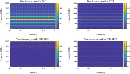
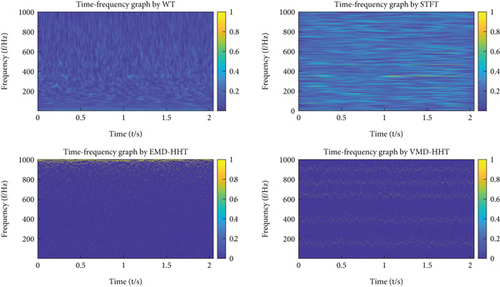
As shown in Figures 4 and 5, the WT and STFT can obtain the resonance frequency and other multiplier frequencies well when there is no noise interference. However, the characteristic frequencies can hardly be obtained by the WT and STFT when the original signals contain strong noise. EMD-HHT can obtain some characteristic frequencies when there is no noise interference, but modal mixing appears when the original signal is doped with noise. The VMD-HHT method can still obtain the frequency characteristics when the signal is dropped with noise. These results indicate that VMD has a strong ability to suppress noise.

The performance of the VMD method was influenced by the preset parameters. The proposed parameter optimization method was applied to the vibration signal with noise to obtain suitable parameters for the VMD. The optimization results were K = 9 and α = 613. The center frequencies by VMD with optimization parameters are compared to the center frequencies by VMD with default parameters (where K = 5 and α = 2000), as shown in Table 1.

Table 1. Decomposition effect comparison of VMD with different parameter settings.

Parameters	Center frequencies of IMFs (Hz)
K = 5, α = 2000	92.70	226.38	359.31	610.80	811.08
K = 9, α = 613	51.81	152.96	260.78	362.56	480.30	584.85	712.40	834.12	953.04

It can be observed that the center frequencies of the IMFs decomposed by the optimization parameters are close to the characteristic frequencies of the vibration signal without noise, as shown in Figure 3. The results indicate that the proposed parameter optimization methods can obtain suitable parameters for VMD, which can help VMD get better performance.

4. Experiment Study

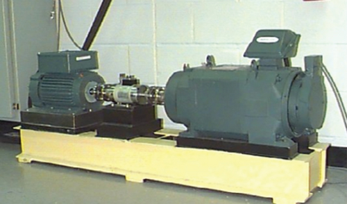
To verify the performance of the proposed method for fault diagnosis, a public bearing dataset from the Bearing Data Centre of the Case Western Reserve University was used [28]. The original datasets can be accessed from https://engineering.case.edu/bearingdatacenter/download-data-file. The experimental platform includes a 2 hp reliance electric motor and data collection device, as shown in Figure 6. The acceleration data of the motor bearing were measured, and the collected dataset contained vibration data under different operating conditions. The signal sampling frequency was 12 kHz, and the rotating speed of the motor was 1772 rpm. The algorithms in this study were run on an Intel i7-6700HQ 2.6 GHz in MATLAB 2022a.

4.1. Fault Diagnosis for Different Fault Types

4.1.1. Analysis of the Influence of Sample Data Length

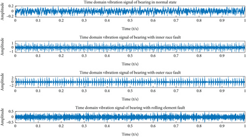
The vibration datasets used in this section contained four different operating conditions: normal, inner race fault, outer race fault, and rolling element fault. The time-domain vibration data are shown in Figure 7. Vibration datasets with different sample lengths were studied to verify the performance of the proposed method, and the sample length was set to 256 points and 1024 points. Because the SVM was applied for classification, the dataset was divided into training and testing sets. The detailed parameters of the vibration datasets are listed in Table 2.

Table 2. The parameters of the vibration datasets for different fault types.

Operating conditions	Sample length	Sample number	Training sample number	Test sample number	Label
Normal	256 data points or 1024 data points	100	50	50	1
Inner race fault			50	50	2
Outer race fault			50	50	3
Rolling fault			50	50	4

The VMD parameters were optimized using the proposed method, and the results were [K = 4, α = 367]. VMD with default parameters [K = 5, α = 2000] was used for future feature calculations of AE, SE, DE, and FDE. These methods were then compared with the proposed method. The detailed parameter settings of the proposed method and comparison methods were referenced to some similar research [21, 25, 29, 30] and are listed in Table 3.

Table 3. The parameter setting of the proposed method and comparison methods.

Method	VMD parameters	Special entropy parameters	Common entropy parameters
VMD+AE	K = 5, α = 2000	Threshold value is 0.15	Embedding value is 2
VMD+SE		Threshold value is 0.15
VMD+DE		Number of classes is 6
VMD+FDE		Number of classes is 6
Proposed method	K = 4, α = 367	Number of classes is 6

Fault diagnosis features were extracted using different methods with data lengths of 256 and 1024 points. The feature contains the entropy of the original vibration signal and the entropy IMFs decomposed by VMD. The mean values and SD of the entropy obtained using different methods are shown in Figure 8.

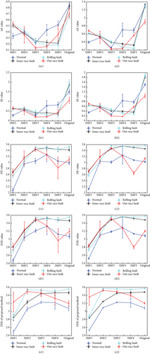
To achieve better diagnostic results, fault diagnosis using entropy values as a fault feature requires significant differences in the entropy values under different operating conditions. As shown in Figure 8, the DE and FDE of the original signal with 1024 data points exhibit significant differences under different operating conditions. However, distinguishability decreased when the data length was reduced to 256. This cannot lead to a better diagnostic result, depending only on the entropy value of the original signal. It can be observed that the entropy of the IMFs by VMD provides more feature information for fault diagnosis. The results indicated that the feature structure proposed in this study can improve the efficiency of fault diagnosis.

As shown in Figure 8, the entropy values of the method proposed in this study have the best differentiation under different operating states, and the standard deviation is small, which is favorable for fault diagnosis. These results indicate that the feature extraction method proposed in this study is effective.

SVM was applied for fault diagnosis based on the above extraction features. The diagnostic accuracy and average calculation time per sample of each method are listed in Table 4.

Table 4. Diagnostic accuracy and average calculation time per sample of each method.

Method	1024 point length		256 point length
Method	Accuracy	Time cost per sample	Accuracy	Time cost per sample
VMD+AE+SVM	99.00%	0.845 s	93.50%	0.169 s
VMD+SE+SVM	99.00%	0.830 s	90.00%	0.166 s
VMD+DE+SVM	100%	0.476 s	97.50%	0.129 s
VMD+FDE+SVM	100%	0.488 s	98.00%	0.131 s
Proposed method	100%	0.670 s	100%	0.165 s

The results presented in Table 4 demonstrate that when the sample data length is 1024 points, the diagnostic accuracy of the various methods is comparatively high, with the DE-based, FDE-based, and proposed methods achieving 100% accuracy. However, the diagnostic efficiency of certain methods decreased when the sample length was reduced to 256 data points. Notably, the efficiency of SE-based fault diagnosis decreased to 90%. However, the diagnostic accuracy of the proposed method remained 100%, which indicates that the proposed method is effective for a short sample length. The calculation times of the proposed method and the comparison methods were approximately equivalent, and the calculation time of the method proposed in this study was acceptable.

4.1.2. Analysis of the Influence of Noise

The influence of noise on the proposed method is analysed in this section. The noise was added to the original vibration signal, and the SNR was set to 5 dB. The sample data length was set to 256 points, and the remaining parameters of the dataset and fault diagnosis methods were set according to Tables 2 and 3.

Fault diagnosis features were extracted using different methods. The feature contains the entropy of the original vibration signal and the entropy IMFs decomposed by VMD. Then the features were applied to SVM for fault diagnosis. The mean values and SD of the entropy obtained by the different methods and the confusion diagrams of the fault diagnosis result are shown in Figure 9.

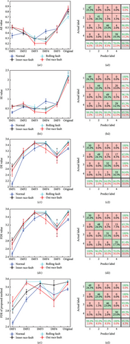
As shown in Figure 9, the features extracted by the proposed method under different operating conditions have more significant discriminability than the features extracted by the other methods. The diagnostic correctness rate of the method proposed in this study reached 95.5%, while the diagnostic correctness rates of the other methods were lower than 87%. The above results demonstrate that the proposed method can achieve good diagnosis results under noise interference.

4.2. Fault Diagnosis for a Single Fault With Different Degrees

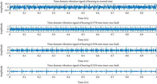
The fault diagnosis for a single fault with different degrees was also presented to verify the proposed fault diagnosis method. The vibration data of the drive end included the normal operation condition and three inner-race fault conditions of 0.1778, 0.3556, and 0.5334 mm. The time-domain vibration data under different conditions are shown in Figure 10. The dataset was built for the analysis in this section according to the parameters listed in Table 5.

Table 5. The parameters of the vibration datasets for inner race fault with diﬀerent degrees.

Operating conditions	Sample length	Sample number	Training sample number	Test sample number	Label
Normal	1024 data points	100	50	50	1
0.1778 mm inner race fault			50	50	2
0.3556 mm inner race fault			50	50	3
0.5334 mm inner race fault			50	50	4

The VMD parameters were optimized using the proposed method, and the results were [K = 6, α = 703]. VMD with default parameters [K = 5, α = 2000] was used for future feature calculations of AE, SE, DE, and FDE. These methods were then compared with the proposed method. The rest of the parameters of the proposed method and comparison methods were set according to Table 3.

The original vibration data were applied directly. Fault diagnosis features were extracted using different methods. The feature contains the entropy of the original vibration signal and the entropy IMFs decomposed by VMD. Then, the features were applied to SVM for fault diagnosis. The mean values and SD of the entropy obtained by the different methods and confusion diagrams of the fault diagnosis results are shown in Figure 11.

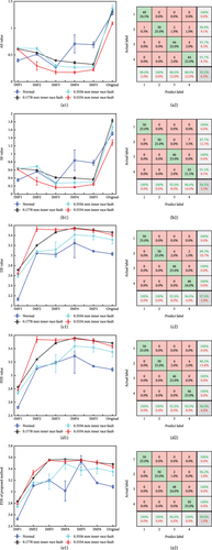
As shown in Figure 11, the features extracted by all methods exhibited good differentiation under different operating conditions. The proposed method and comparison methods performed well for both the normal state and the 0.1778 inner race fault state; only one misdiagnosis occurred in the AE-based method. Most misdiagnoses occurred in the 0.3556 mm inner race fault and 0.5334 mm inner race fault states. The proposed method achieved better diagnosis results in this part; only two misdiagnoses occurred, and the accuracy rate of the fault diagnosis reached 99%. The results demonstrate that the proposed method has good diagnostic ability.

A dataset with additional noise was used for fault diagnosis. The noise was added to the original vibration signal, and the SNR was set to 5 dB. The mean values and SD of the entropy obtained by the different methods and confusion diagrams of the fault diagnosis results are shown in Figure 12.

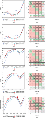
As shown in Figure 12, the differentiation of the four operating condition features decreased for all the methods under noise interference, and the features extracted based on DE and FDE performed better than AE and SE. Most misdiagnoses still occurred in the 0.3556 mm inner race fault and 0.5334 mm inner race fault states. The proposed method obtained the highest fault-diagnosis accuracy of 94%. The results indicate that the proposed method has a good fault diagnosis ability under noise interference.

All the above experimental study results indicate that the proposed fault diagnosis method has good performance for the fault diagnosis of rolling bearings. In addition, the proposed method exhibits a better fault diagnosis effect when the sample data length is short and mixed with noise.

5. Conclusions

Reasonable data processing can obtain effective features to improve fault diagnosis. VMD is a useful data processing method for nonstationary vibration signals, and the FDE of vibration data can express the state change of the rolling bearing. However, the preparameter setting of VMD influences the decomposition performance, and a single entropy cannot present complete features. Therefore, parameter optimization of VMD based on SSA and a new fitness function based on FDE is proposed to obtain more useful features for fault diagnosis in this study. Based on the results of the experimental studies, the following conclusions were drawn.

a.
The proposed feature extraction method based on VMD with parameter optimization and FDE is efficient for fault diagnosis of rolling bearings.
b.
The proposed feature extraction method can obtain useful features for fault diagnosis, particularly in short-length samples and noise conditions.
c.
The proposed method performed well in fault diagnosis for different fault types and degrees.

Conflicts of Interest

The authors declare no conflicts of interest.

Funding

This work is supported by the Suqian Sci&Tech Program (Grant No. H202410) and the National Natural Science Foundation of China (NSFC) (51709121).

Acknowledgments

This work is supported by the Suqian Sci&Tech Program (Grant No. H202410) and the National Natural Science Foundation of China (NSFC) (51709121).

Open Research

Data Availability Statement

The data that support the findings of this study are available upon request from the corresponding author.

References

1 Li Z., Jiang H., and Liu Y., A reinforcement double deep Q-network with prioritised experience replay for rolling bearing fault diagnosis, Measurement Science & Technology. (2023) 34, no. 12, 125133, https://doi.org/10.1088/1361-6501/acf23d.
10.1088/1361-6501/acf23d
CAS Web of Science® Google Scholar
2 Huang Y., Zhang W., Wang K., Zhang B., Zhang F., and Luo H., Fault diagnosis of low-speed rolling bearing based on weighted reconstruction of vibration envelopes, Wind Energy. (2023) 26, no. 7, 637–649, https://doi.org/10.1002/we.2820.
10.1002/we.2820
Web of Science® Google Scholar
3 Liu H., Li L., and Ma J., Rolling bearing fault diagnosis based on STFT-deep learning and sound signals, Shock and Vibration. (2016) 2016, no. 1, 6127479, https://doi.org/10.1155/2016/6127479, 2-s2.0-84988723839.
10.1155/2016/6127479
Web of Science® Google Scholar
4 Jakubek B., Grochalski K., Rukat W., and Sokol H., Thermovision measurements of rolling bearings, Measurement. (2022) 189, 110512, https://doi.org/10.1016/j.measurement.2021.110512.
10.1016/j.measurement.2021.110512
Web of Science® Google Scholar
5 Wang H. and Chen P., A feature extraction method based on information theory for fault diagnosis of reciprocating machinery, Sensors. (2009) 9, no. 4, 2415–2436, https://doi.org/10.3390/s90402415, 2-s2.0-63849187550, 22574021.
10.3390/s90402415
PubMed Web of Science® Google Scholar
6 Jiang Z., Zhang K., Xiang L., and Xu Y., Differential spectral amplitude modulation and its applications in rolling bearing fault diagnosis, Measurement. (2022) 201, 111755, https://doi.org/10.1016/j.measurement.2022.111755.
10.1016/j.measurement.2022.111755
Web of Science® Google Scholar
7 Kankar P. K., Sharma S. C., and Harsha S. P., Fault diagnosis of ball bearings using machine learning methods, Expert Systems with Applications. (2011) 38, no. 3, 1876–1886, https://doi.org/10.1016/j.eswa.2010.07.119, 2-s2.0-78049528234.
10.1016/j.eswa.2010.07.119
Web of Science® Google Scholar
8 Yi J., Tan H., Yan J., and Chen X., Adaptive rotating machinery fault diagnosis method using MKIST, Measurement Science & Technology. (2024) 35, no. 4, 045010, https://doi.org/10.1088/1361-6501/ad1c49.
10.1088/1361-6501/ad1c49
CAS Web of Science® Google Scholar
9 Alexakos C. T., Karnavas Y. L., Drakaki M., and Tziafettas I. A., A combined short time Fourier transform and image classification transformer model for rolling element bearings fault diagnosis in electric motors, Machine Learning and Knowledge Extraction. (2021) 3, no. 1, 228–242, https://doi.org/10.3390/make3010011.
10.3390/make3010011
Web of Science® Google Scholar
10 Kankar P. K., Sharma S. C., and Harsha S. P., Fault diagnosis of ball bearings using continuous wavelet transform, Applied Soft Computing. (2011) 11, no. 2, 2300–2312, https://doi.org/10.1016/j.asoc.2010.08.011, 2-s2.0-78751629036.
10.1016/j.asoc.2010.08.011
Web of Science® Google Scholar
11 Zhou Y., Wigner–Ville distribution based on cyclic spectral density and the application in rolling element bearings diagnosis, Proceedings of the Institution of Mechanical Engineers, Part C: Journal of Mechanical Engineering Science. (2011) 225, no. 12, 2831–2847, https://doi.org/10.1177/0954406211413215, 2-s2.0-84863059358.
10.1177/0954406211413215
Web of Science® Google Scholar
12 Zhuang X., Yang C., Yang J., Wu C., Shan Z., and Gong T., Rolling bearing fault diagnosis by aperiodic stochastic resonance under variable speed conditions, Fluctuation and Noise Letters. (2022) 21, no. 2, https://doi.org/10.1142/S0219477522500158.
10.1142/S0219477522500158
Web of Science® Google Scholar
13 Ben Ali J., Fnaiech N., Saidi L., Chebel-Morello B., and Fnaiech F., Application of empirical mode decomposition and artificial neural network for automatic bearing fault diagnosis based on vibration signals, Applied Acoustics. (2015) 89, 16–27, https://doi.org/10.1016/j.apacoust.2014.08.016, 2-s2.0-84907486966.
10.1016/j.apacoust.2014.08.016
Web of Science® Google Scholar
14 Sahu P. K. and Rai R. N., Fault diagnosis of rolling bearing based on an improved denoising technique using complete ensemble empirical mode decomposition and adaptive thresholding method, Journal of Vibration Engineering & Technologies. (2023) 11, no. 2, 513–535, https://doi.org/10.1007/s42417-022-00591-z.
10.1007/s42417-022-00591-z
Web of Science® Google Scholar
15 Dragomiretskiy K. and Zoss D., Variational mode decomposition, IEEE Transactions on Signal Processing. (2014) 62, no. 3, 531–544, https://doi.org/10.1109/TSP.2013.2288675, 2-s2.0-84893418756.
10.1109/TSP.2013.2288675
Web of Science® Google Scholar
16 Zhu K. and Song X., Cross-fuzzy entropy-based approach for performance degradation assessment of rolling element bearings, Proceedings of the Institution of Mechanical Engineers, Part E: Journal of Process Mechanical Engineering. (2018) 232, no. 2, 173–185, https://doi.org/10.1177/0954408917691072, 2-s2.0-85042350539.
10.1177/0954408917691072
Web of Science® Google Scholar
17 Barszcz T. and Sawalhi N., Fault detection enhancement in rolling element bearings using the minimum entropy deconvolution, Archives of Acoustics. (2012) 37, no. 2, 131–141, https://doi.org/10.2478/v10168-012-0019-2, 2-s2.0-84864116161.
10.2478/v10168-012-0019-2
Web of Science® Google Scholar
18 Chao Z. and Jianjun C., Diagnosing faults of bearings with LMD approximate entropy and SVM, Mechanical Science and Technology for Aerospace Engineering. (2012) 31, no. 9, 1539–1548.
Google Scholar
19 Li Y. and Zhou X., Rolling bearing fault diagnosis based on HVD algorithm and sample entropy, Journal of Computational Methods in Sciences and Engineering. (2019) 19, no. 6, 331–340, https://doi.org/10.3233/JCM-191048, 2-s2.0-85071673809.
10.3233/JCM-191048
Google Scholar
20 Li Y., Zhang W., Xiong Q., Luo D., Mei G., and Zhang T., A rolling bearing fault diagnosis strategy based on improved multiscale permutation entropy and least squares SVM, Journal of Mechanical Science and Technology. (2017) 31, no. 6, 2711–2722, https://doi.org/10.1007/s12206-017-0514-5, 2-s2.0-85021199793.
10.1007/s12206-017-0514-5
Web of Science® Google Scholar
21 Rostaghi M. and Azami H., Dispersion entropy: a measure for time-series analysis, IEEE Signal Processing Letters. (2016) 23, no. 5, 610–614, https://doi.org/10.1109/LSP.2016.2542881, 2-s2.0-84964343754.
10.1109/LSP.2016.2542881
Web of Science® Google Scholar
22 Tong Y. H., Ling G., Guan Z. H., Fan Q., and Wan L., Refined composite multiscale phase Rényi dispersion entropy for complexity measure, International Journal of Bifurcation and Chaos. (2023) 33, no. 5, 2350054, https://doi.org/10.1142/S0218127423500542.
10.1142/S0218127423500542
Web of Science® Google Scholar
23 Feng Z., Liang M., Zhang Y., and Hou S., Fault diagnosis for wind turbine planetary gearboxes via demodulation analysis based on ensemble empirical mode decomposition and energy separation, Renewable Energy. (2012) 47, 112–126, https://doi.org/10.1016/j.renene.2012.04.019, 2-s2.0-84860824316.
10.1016/j.renene.2012.04.019
Web of Science® Google Scholar
24 Xiaoan Y., Xing H., Dong J., and Ling X., A novel robust intelligent fault diagnosis method for rolling bearings based on SPAVMD and WOA-LSSVM under noisy conditions, Measurement Science & Technology. (2024) 35, no. 5, 056121, https://doi.org/10.1088/1361-6501/ad29e3.
10.1088/1361-6501/ad29e3
Google Scholar
25 Mostafa R., Mohammad M. K., Mohammad R. A., and Hamed A., Fuzzy dispersion entropy: a nonlinear measure for signal analysis, IEEE Transactions on Fuzzy Systems. (2022) 30, no. 9, 3785–3796.
10.1109/TFUZZ.2021.3128957
Google Scholar
26 Yun P., Zhou Y., Liu C., Wu Y., and Pan D., Forecasting China carbon price using an error-corrected secondary decomposition hybrid model integrated fuzzy dispersion entropy and deep learning paradigm, Environmental Science and Pollution Research. (2024) 31, no. 11, 16530–16553, https://doi.org/10.1007/s11356-024-32169-5, 38321281.
10.1007/s11356-024-32169-5
PubMed Web of Science® Google Scholar
27 Xue J. K. and Shen B., A novel swarm intelligence optimization approach: sparrow search algorithm, Systems Science & Control Engineering. (2020) 8, no. 1, 22–34, https://doi.org/10.1080/21642583.2019.1708830.
10.1080/21642583.2019.1708830
Web of Science® Google Scholar
28 Jin Z. and Sun Y., Bearing fault diagnosis based on VMD fuzzy entropy and improved deep belief networks, Journal of Vibration Engineering & Technologies. (2023) 11, no. 2, 577–587, https://doi.org/10.1007/s42417-022-00595-9.
10.1007/s42417-022-00595-9
Web of Science® Google Scholar
29 Bian X. and Zhang J., Bearing fault diagnosis based on LMD approximate entropy and improved PSO-ELM, Machine Tool & Hydraulics. (2023) 51, no. 14, 227–232.
Google Scholar
30 Liu J. C., Quan H., Yu X., He K., and Li Z. H., Rolling bearing fault diagnosis based on parameter optimization VMD and sample entropy, Acta Automatica Sinica. (2019) 48, no. 3, 808–819.
Google Scholar

All articles

A Hybrid Fault Diagnosis Model for Rolling Bearing With Optimized VMD and Fuzzy Dispersion Entropy

Abstract

1. Introduction