The Painlevé equations and their series and rational solutions are essential in applied, pure mathematics and theoretical physics. Recently, quantum algorithms have helped to implement numerical algorithms more easily by performing linear algebra in our working. This article uses a hybrid of quantum computing schemes and spectral methods for the second Painlevé equation. Two approaches are investigated: first, a series solution is obtained, and then the rational solutions. The successive linearization method is used for the linearization of the Painlevé-II equation. In the computer implementation, the solution value of the Painlevé-II equation is considered as a final quantum state. In each iterative scheme, by adding the current quantum state, we can compute the final quantum state. We need different quantum models for each approach, series, and rational solutions. Numerical examples illustrate the efficiency of this method, and reasonable solutions are obtained for a wide range of parameter values.

1. Introduction

In the years 1895–1910, Painlevé and Gambier investigated the famous nonlinear second-order differential equation:

(1)

where R is a holomorphic function in t and rational in w and w^′. It can be proved that this equation has the Painlevé property, and it means that the only moveable singularities are poles. Painlevé explained the solutions of (1) in terms of classical special functions or elliptic functions, except in six cases which are irreducible and required new special functions to obtain the solutions [1]. In this work, the second kind of the Painlevé equation is

(2)

where α is a known parameter considered. This equation can be obtained from the Korteweg–de Vries (KdV) equation and has many applications in physics, describing the electric field in a semiconductor, plasma physics, statistical mechanics, quantum gravity, general relativity, nonlinear waves, fiber optics, and nonlinear optics [2–4]. In recent years, many researchers have tried to solve this equation through many methods. For example, solving (2) with the initial conditions,

(3)

by the analytic continuation method [5], the Adomian’s decomposition method [6], the homotopy analysis method (HAM) [7], the Sinc-collocation method, the variational iteration method (VIM) [8], the optimal homotopy asymptotic method (OHAM) [9], and the variational auxiliary parameter (VAP) [10].

Spectral methods have an important role in solving engineering problems such as differential equations, with efficient and accurate numerical solutions (see [11, 12]) and many other books in this topic. By the combination of spectral methods and a mesh-free approach, many problems can be solved [13, 14]. Very recently, Taema and Youssri have developed a spectral collocation method by using third-kind Chebyshev polynomials to solve a system of two nonlinear integrodifferential equations that arise in biological modeling [15]. Youssri and Atta have proposed a novel spectral algorithm utilizing Fibonacci polynomials to numerically solve both linear and nonlinear integrodifferential equations with fractional-order derivatives [16].

In this article, a quantum pseudospectral method (QPSM) for the nonlinear second kind Painlevé equation (1) is considered; very recently, this method has been used for solving the general Lane–Emden type equations [17]. The author believes that it is the first attempt to find the series and rational solution for the Painlevé-II equation with the quantum pseudo-spectral method. Two approaches are studied. In the first attempt, the governing equation (2) for t ∈ [0, 1] with the initial conditions (2) is considered. In the second attempt, the rational solutions of the second kind Painlevé equation are considered. The QPSM by using the quantum linear system algorithm (QLSA) [18] is designed for linear initial value problems (IVP) [19]. The quantum algorithm in [19] is based on a pseudo-spectral method for time-dependent IVP with the polynomial complexity.

Suppose the unknown function w(.) for i ∈ [M] = {1, 2, …, M} has the following expression:

(4)

with the unknown W_i(.) and w_k(.) as the successive approximation solutions that are obtained recursively by applying the QPSM on the linearized form of equation (2) after substituting (4), where M is the number of iterations. By simple calculating, we have

(5)

Let w₀(.) be an initial approximation that satisfies the initial conditions in (3), for example

(6)

Also, we assumed that lim_i⟶∞ W_i = 0. Then, for i ∈ [M], w_i(.) is computed by solving the linearization form of (5) iteratively. It means the linear IVP

(7)

where

(8)

with

should be solved, where M is the order of the QPSM. Similar to [17], the IVP (6) converts to a system of ordinary differential equations (ODEs):

(9)

with the conditions z_i,0(0) = z_i,1(0) = 0, z_i,0 = w_i, and

. By (9), the coefficient matrix is defined as follows:

(10)

Now, we want to use the pseudospectral method by using the Chebyshev polynomials [11, 20]. By applying the truncated Chebyshev polynomial approximation for (7), we have for v ∈ {0, 1}

(11)

for any

and also for s ∈ [−1, 1],

(12)

In (11), s ∈ [−1, 1] and hence later we rescale the range of the independent variable in (2) to [−1, 1]. We use the Chebyshev–Gauss–Lobatto quadrature nodes, s_k = cos((kπ)/n) for k ∈ [n + 1]₀ = {0, 1, …, n}, to solve the linear system obtained from (9). For calculating c_i,v,l, let us consider

(13)

with

(14)

and the coefficients of the upper triangular matrix D_n are [12]

(15)

and

(16)

Hence, by (9) and (11) for k ∈ [n + 1]₀ and i ∈ [M], we have

(17)

In our approach, the linear system (17) is solved by the QLSA. Now, to improve the accuracy of the domain of (2), it is divided into m subintervals

(18)

with Ψ₀ = 0, Ψ_m = 1. Each subinterval [Ψ_q, Ψ_q+1] for q ∈ [m]₀ rescaled onto [−1, 1]. Let Δ_q = 1/m = Ψ_q+1 − Ψ_q. Hence, t ∈ [0, 1] converts to s ∈ [−1, 1] with

(19)

and hence,

(20)

After rescaling (7), then (9) converts to

(21)

where

(22)

and C = (ds/dt) and y_i,q,v(s) = z_i,v(t) = z_i,v(IK_q(s)) for t ∈ [Ψ_q, Ψ_q+1], v ∈ {0, 1}, q ∈ [m]₀, and i ∈ [M]. By (21), the coefficient matrix is defined as follows:

(23)

2. QPSM

For a better understanding of quantum computing symbols, see [21]. As discussed in the previous section, we should solve a linear system like

(24)

in each iteration by the QLSA presented in [19] from the linear equation (21). The vector

(25)

describes the solution by

(26)

where c_i,ρ,k(Ψ_q+1) is the coefficient of Chebyshev expansion of y_i,q,ρ(K_q(Ψ_q+1)), x_iρ is the last state y_i,m−1,ρ(K_q(Ψ_m)), and p is a padding trick [18, 22]. We require

as the output at t = 1 because w₀(1) = 1 + α/2.

The elements of L_i and B_i are computed according to the QPSM by the flowchart described in Figure 1, [17]. It can be proved that for the linear system (21), we have

(27)

Details are in the caption following the image — **Figure 1**
Open in figure viewer PowerPoint

Flowchart steps in the quantum pseudospectral method.

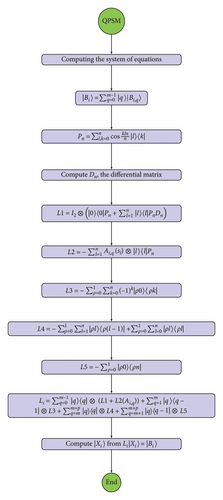
In continuation, the total error in this method is explained. A part of the error is due to the linearization of equation (5). Remarks 1 and 3 explain this. Another part of the error is related to the pseudo-spectral method (see Lemma 1).

Remark 1. The error generated in (7) is due to

(28)

and the linearization error is bounded by

. Hence, for a sufficiently large M, we should have W_i⟶0 in the convergence case.

Remark 2. With respect to (5) and (6), obviously error in (28) in the i^th iteration is

(29)

Lemma 1 (see [23].)For the linear system L_i|X_i〉 = |B_i〉 in (24), let y_i and be the approximate and exact ODE solutions, respectively, in each iteration. Then, for sufficiently large n, at the time T, the L² norm of the error satisfies

(30)

3. Results and Discussion

Some examples with different α in (2) for showing accuracy and comparing with other methods are considered. In all examples, we put p = 1, and Python 3.12.4 is used for programming. Algorithm 1 shows the description of this method.

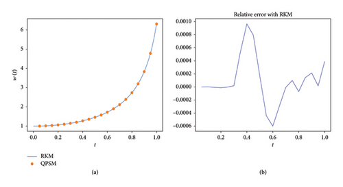
In the first attempt, we consider α = 1 in the second Painlevé equation (2). Figure 2(a) shows results of the QPSM for n = m = 20 with M = 5, and the right figure shows the relative absolute error of the QPSM concerning the Runge–Kutta method (RKM) [24] with atol = 0.00000001 (absolute tolerances). Table 1 shows a comparison between the QPSM, the RKM, the Sinc-collocation method [8], the VIM [25], the OHAM [9], the VAP [10], and the Legendre τ-decomposition method (LTM) [6].

Table 1. Comparison of the values of w(t) by different methods at α = 1.

t	QPSM	RKM	Sinc	VIM	OHAM	VAP	LTM
0.1	1.01524354	1.01524596	1.015243802	1.015243537	1.01697332	1.015	1.01525769
0.2	1.06261465	1.06260244	1.062615730	1.062614651	1.06804971	1.063	1.06259868
0.3	1.14637603	1.14639773	1.146377520	1.146376034	1.15463133	1.146	1.14638761
0.4	1.27415229	1.27538325	1.274150163	1.274152278	1.28209418	1.275	1.27413995
0.5	1.45921345	1.45945595	1.459216534	1.459213319	1.46396018	1.468	1.45923019
0.6	1.72537555	1.72434098	1.725383228	1.725374098	1.72697690	1.743	1.72535520
0.7	2.11844345	2.11843013	2.118441811	2.118431139	2.11915382	2.156	2.11846104
0.8	2.73693513	2.73674274	2.736942571	2.736846427	2.73683163	2.806	2.73693516
0.9	3.84437392	3.83519858	3.834408328	3.833780746	3.83251635	3.934	3.83437316
1.0	6.30892109	6.31139164	—	—	—	6.259	—

Algorithm 1: QPSM algorithm for finding the series solution of the Painlevé-II equation.

Input:M = 5, n = m = 20, p = 1 and initial approximation w₀(t) = (α/2)t² + 1.
Output:w(1)
1.
y = y_Initial = w₀(1)
2.
fori⟵1 to Mdo
3.
Compute L1, L2, L3, L4, L5 in Section 2 // for computing L_i in (24)
4.
Compute B_i, right-hand side of (24)
5.
Compute , the solution of (24)
6.
Extract x_i0 from X_i // (2m(n + 1) + 1)^th vector component
7.
y⟵y + x_i0
8.
returny

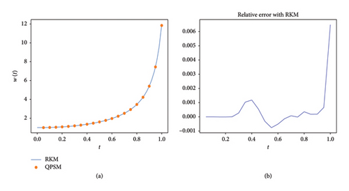
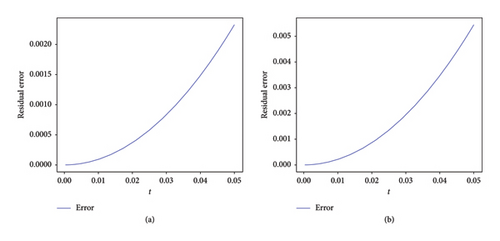
Figure 3(a) shows results of the QPSM for α = 2 and n = m = 20 with M = 5, and the right figure shows the relative absolute error of the QPSM concerning the RKM [24] with atol = 0.00000001 (absolute tolerances). Table 2 shows a comparison between the QPSM, the RKM, Adomian’s decomposition method (ADM) [7], theLTM [6], the Sinc-collocation method, and VIM coupled with Padé approximation (VIPA) [8]. Figure 4 show the residual error in first partition for M = 5 and n = m = 20. The results show the efficiency of the QPSM.

Table 2. Comparison of the values of w(t) by different methods at α = 2.

t	QPSM	RKM	ADM	LTM	Sinc	VIPA
0.1	1.02026919	1.02027074	1.020269194	1.021047331	1.020269516	1.020269194
0.2	1.08304976	1.08303857	1.083049760	1.082116225	1.083050684	1.083049760
0.3	1.19379025	1.19410929	1.193790245	1.194531584	1.193791418	1.193790245
0.4	1.36282365	1.36443616	1.362823651	1.361992274	1.362825244	1.362823638
0.5	1.60929104	1.60878420	1.609291039	1.610416473	1.609294013	1.609290816
0.6	1.97019075	1.96918366	1.970190748	1.968817717	1.970195495	1.970188429
0.7	2.52374240	2.52393387	2.523742462	2.525021861	2.523748780	2.523724908
0.8	3.46221940	3.46346053	3.462223434	3.461891692	3.462235205	3.462114640
0.9	5.40216795	5.40317736	5.402303840	5.400956596	5.402575104	5.401914998
1.0	11.84754955	11.92435805	—	—	—	—

4. Approximating the Rational Solutions

As we said before, the second Painlevé equation (2) has many interesting properties such as the Painlevé property, which means that the only moveable singularities are poles [1], and by the Lax pair, we can solve the Cauchy problem for this equation [26]. It can be proved that this equation has exactly one rational solution if and only if . Some rational solutions are listed in Table 3, [1].

Table 3. List of rational solutions of the second Painlevé equation (2).

α	w(t)
0	0
±1	∓1/t
±2	±(4 − 2t³)/(4t + t⁴)
±3	∓(3t²(160 + 8t³ + t⁶))/(−320 + 24t⁶ + t⁹)
±4	∓(4(−22400 − 112000t³ − 22400t⁶ + 1000t⁹ + 50t¹² + t¹⁵))/(t(−80 + 20t³ + t⁶)(11200 + 60t⁶ + t⁹))

Remark 3 (see [1].)Let w(.) be the rational solution of the second Painlevé equation (2) with α ≠ 0 and n₊, n₋ be the number of poles with residue +1 and −1, respectively. Then, n₊ = α(α − 1)/2 and n₋ = α(α + 1)/2, and hence, n₊ + n₋ = α². Moreover, there exists a rational function such as F(.) such that tw(t) = F(t³).

Remark 4 (see [3].)By Bäcklund transformation and for α ≠ ±1/2, we have

(31)

where w(t, α) is the solution of (2).

In continuation, we try to show the power of the QPSM to find the rational solutions of the second Painlevé equation (2) with α ≠ 0. Because of Remarks 3 and 4, we consider the Painlevé equation (2) for a region that does not contain origin, like t ∈ [1, 2]. Any rational solution w(t) of (2) can be written as the quotient of two entire functions, like w(t) = (v(t)/u(t)), and this representation is not unique. In this case, the entire functions v(.) and u(.) should satisfy [1],

(32)

Now, we have a system of nonlinear ODEs with two equations and two unknown functions v(.) and u(.), and in continuation, these functions are obtained by the QPSM.

Suppose the unknown functions v(.) and u(.) can be expanded as

(33)

with the unknowns V_i(.) and U_i(.) and v_k(.) and u_k(.) as the successive approximation solutions that are obtained recursively by applying the QPSM on the linearized form of equation (32) after substituting (33). Hence, we have

(34)

It can be shown that the system (34) linearized as

(35)

After constructing subintervals and rescaling (like (21)), the system (35) converts to

(36)

where

(37)

and like before C = (ds/dt), y_i,q,ρ(s) = u_i,ρ(t) = u_i,ρ(IK_q(s)) for ρ ∈ {0, 1}, y_i,q,ρ(s) = v_i,ρ(t) = v_i,ρ(IK_q(s)) for ρ ∈ {2, 3}, t ∈ [Ψ_q, Ψ_q+1], q ∈ [m]₀, and i ∈ [M].

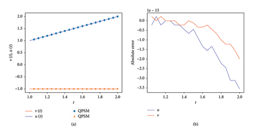
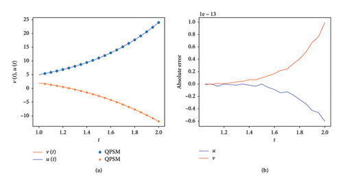
In continuation, we test the QPSM for (36) with α = 1, and with the help of Remarks 3 and 4, we take v₀(t) = −1 and u₀(t) = (1 + t²)/2. Figure 5(a) shows QPSM’s results for α = 1 and n = m = 20, with M = 5, and the right figure shows the absolute error of the QPSM concerning Table 3. Figure 6 show the results of the QPSM for α = 2 and m = n = 20, with 5 iterations (M = 5). In two examples, we see the efficiency of the QPSM.

5. Conclusions

One of the main advantages of the QSPM is its applicability to linear and nonlinear ODEs. The QPSM can be implemented on linear ODEs very easily, but nonlinear ODEs are not straightforward. Finding a suitable linearized form of nonlinear ODEs and finding the initial guess are not easy. This article proposes a novel approach based on quantum computing to solve the second Painlevé equation. These models have high nonlinearity. Two approaches are investigated: first, a series solution is obtained, and then the rational solutions. The nonlinear equations are linearized using the successive linearization method. In all examples, the comparisons with numerical and semianalytical methods show the efficiency of the results. The accurate results are obtained by choosing suitable parameter values. Given the capabilities of quantum algorithms, their implementation on fractional differential equations is not out of the question and could yield interesting results in this field in the future.

Conflicts of Interest

The author declares no conflicts of interest.

Funding

No funding was received for this research.

Open Research

Data Availability Statement

The data that support the findings of this study are available from the corresponding author upon reasonable request.

References

1 Gromak V. I., Laine I., and Shimomura S., Painlevé Differential Equations in the Complex Plane, De Gruyter Studies in Mathematics. (2002) Walter de Gruyter, Berlin, New York.
Google Scholar
2 Abdullayev A. S., Pure Imaginary Solutions of the Second Painlevé Equation, International Journal of Mathematics and Mathematical Sciences. (2004) 2004, no. 56.
10.1155/S0161171204310070
Google Scholar
3 Clarkson P. A., Painlevé Equations—Nonlinear Special Functions, Journal of Computational and Applied Mathematics. (2003) 153, no. 1-2, 127–140, https://doi.org/10.1016/s0377-0427(02)00589-7, 2-s2.0-0037380208.
10.1016/S0377-0427(02)00589-7
Web of Science® Google Scholar
4 Kudryashov N. A., The Second Painlevé Equation as a Model for the Electric Field in a Semiconductor, Physics Letters A. (1997) 233, no. 4-6, 397–400, https://doi.org/10.1016/s0375-9601(97)00545-8, 2-s2.0-0008117890.
10.1016/S0375-9601(97)00545-8
CAS Web of Science® Google Scholar
5 Davis H. T., Introduction to Non-Linear Differential and Integral Equations, 1962, Journal of the London Mathematical Society.
Google Scholar
6 Dehghan M. and Shakeri F., The Numerical Solution of the Second Painlevé Equation, Numerical Methods for Partial Differential Equations. (2009) 25, no. 5, 1238–1259, https://doi.org/10.1002/num.20416, 2-s2.0-67651223722.
10.1002/num.20416
Web of Science® Google Scholar
7 Ellahi R., Abbasbandy S., Hayat T., and Zeeshan A., On Comparison of Series and Numerical Solutions for Second Painlevé Equation, Numerical Methods for Partial Differential Equations. (2010) 26, no. 5, 1070–1078, https://doi.org/10.1002/num.20475, 2-s2.0-77956207513.
10.1002/num.20475
Web of Science® Google Scholar
8 Saadatmandi A., Numerical Study of Second Painlevé Equation, Communications in Numerical Analysis. (2012) 2012.
10.5899/2012/cna-00157
Google Scholar
9 Sierra-Porta D., Some Algebraic Approach for the Second Painlevé Equation Using the Optimal Homotopy Asymptotic Method (OHAM), Numerical Analysis and Applications. (2018) 11, no. 2, 170–177, https://doi.org/10.1134/s1995423918020076, 2-s2.0-85048196045.
10.1134/S1995423918020076
Google Scholar
10 Ahmad H., Khan T. A., and Yao S. W., Numerical Solution of Second Order Painlevé Differential Equation, The Journal of Mathematics and Computer Science. (2020) 21, 150–157.
10.22436/jmcs.021.02.06
Google Scholar
11 Shen J., Tang T., and Wang L. L., Spectral Methods: Algorithms, Analysis and Applications, 2011, Springer.
10.1007/978-3-540-71041-7
Web of Science® Google Scholar
12 Trefethen L. N., Spectral Methods in Matlab, 2000, Society for Industrial and Applied Mathematics (SIAM).
10.1137/1.9780898719598
Google Scholar
13 Abbasbandy S., Shivanian E., and Al-Jizani K. H., On the Analysis of a Kind of Nonlinear Sobolev Equation Through Locally Applied Pseudo-spectral Meshfree Radial Point Interpolation, Numerical Methods for Partial Differential Equations. (2012) 37, no. 1, 462–478.
10.1002/num.22536
Google Scholar
14 Shivanian E. and Abbasbandy S., Pseudospectral Meshless Radial Point Interpolation for Generalized Biharmonic Equation in the Presence of Cahn–Hilliard Conditions, Computational and Applied Mathematics. (2020) 39, no. 3, https://doi.org/10.1007/s40314-020-01175-x.
10.1007/s40314-020-01175-x
Google Scholar
15 Taema M. A. and H Youssri Y., Third-Kind Chebyshev Spectral Collocation Method for Solving Models of Two Interacting Biological Species, Contemporary Mathematics. (2024) 5, no. 4, 6189–6207, https://doi.org/10.37256/cm.5420245950.
10.37256/cm.5420245950
Google Scholar
16 Youssri Y. H. and Atta A. G., Fejér-Quadrature Collocation Algorithm for Solving Fractional Integro-Differential Equations via Fibonacci Polynomials, Contemporary Mathematics. (2024) 5, no. 1, 296–308, https://doi.org/10.37256/cm.5120244054.
10.37256/cm.5120244054
Google Scholar
17 Abbasbandy S., A Hybrid Quantum-Spectral-Successive Linearization Method for General Lane-Emden Type Equations, Journal of Applied Mathematics and Computing. (2024) 71, no. 2, 1581–1607, https://doi.org/10.1007/s12190-024-02290-2.
10.1007/s12190-024-02290-2
Google Scholar
18 Harrow A. W., Hassidim A., and Lloyd S., Quantum Algorithm for Linear Systems of Equations, Physical Review Letters. (2009) 103, no. 15, https://doi.org/10.1103/physrevlett.103.150502, 2-s2.0-70349862042.
10.1103/PhysRevLett.103.150502
PubMed Google Scholar
19 Childs A. M. and Liu J. P., Quantum Spectral Methods for Differential Equations, Communications in Mathematical Physics. (2020) 375, no. 2, 1427–1457, https://doi.org/10.1007/s00220-020-03699-z.
10.1007/s00220-020-03699-z
Web of Science® Google Scholar
20 Hosseini M. M., A Modified Pseudospectral Method for Numerical Solution of Ordinary Differential Equations Systems, Applied Mathematics and Computation. (2006) 176, no. 2, 470–475, https://doi.org/10.1016/j.amc.2005.09.036, 2-s2.0-33646371956.
10.1016/j.amc.2005.09.036
Google Scholar
21 Zygelman B., A First Introduction to Quantum Computing and Information, 2018, Springer.
10.1007/978-3-319-91629-3
Google Scholar
22 Berry D. W., Childs A. M., Ostrander A., and Wang G., Quantum Algorithm for Linear Differential Equations With Exponentially Improved Dependence on Precision, Communications in Mathematical Physics. (2017) 356, no. 3, 1057–1081, https://doi.org/10.1007/s00220-017-3002-y, 2-s2.0-85030661144.
10.1007/s00220-017-3002-y
Web of Science® Google Scholar
23 Gheorghiu C. I., Spectral Methods for Differential Problems. Casa Cartii de Stiinta, 2007, Publishing House.
Google Scholar
24 Dormand J. R. and Prince P. J., A Family of Embedded Runge-Kutta Formulae, Journal of Computational and Applied Mathematics. (1980) 6, no. 1, 19–26, https://doi.org/10.1016/0771-050x(80)90013-3, 2-s2.0-0018991720.
10.1016/0771-050X(80)90013-3
Google Scholar
25 Abbasbandy S., An Approximation Solution of a Nonlinear Equation With Riemann-Liouville’s Fractional Derivatives by He’s Variational Iteration Method, Journal of Computational and Applied Mathematics. (2007) 207, no. 1, 53–58, https://doi.org/10.1016/j.cam.2006.07.011, 2-s2.0-34250647432.
10.1016/j.cam.2006.07.011
Web of Science® Google Scholar
26 Kudryashov N. A., Rational Solutions of Equations Associated with the Second Painlevé Equation, Regular & Chaotic Dynamics. (2020) 25, no. 3, 273–280, https://doi.org/10.1134/s156035472003003x.
10.1134/S156035472003003X
Google Scholar

All articles

Series and Rational Solutions of the Second Kind Painlevé Equations by Using the Quantum Pseudospectral Method

Abstract

1. Introduction

2. QPSM

3. Results and Discussion

4. Approximating the Rational Solutions

5. Conclusions

Conflicts of Interest

Funding

Open Research

Data Availability Statement

References

Figures

References

Information

About Wiley Online Library

Help & Support

Opportunities

Connect with Wiley

Series and Rational Solutions of the Second Kind Painlevé Equations by Using the Quantum Pseudospectral Method

Abstract

1. Introduction

2. QPSM

3. Results and Discussion

4. Approximating the Rational Solutions

5. Conclusions

Conflicts of Interest

Funding

Open Research

Data Availability Statement

References

Figures

References

Related

Information