The combination of evolutionary algorithms with full-wave electromagnetic (EM) simulation software is an effective method for antenna optimal design. However, the high computational cost of calling the full-wave EM simulation hundreds or thousands of times makes it unacceptable in terms of design time. In recent research, machine learning (ML) methods have achieved considerable success as surrogate models replacing full-wave EM simulation software. Among them, the selection and construction of surrogate models are key factors. This paper proposes a skip-connected surrogate model based on convolutional neural network (CNN) and Bayesian neural network (BNN). Firstly, transfer learning is employed to combine the spatial feature extraction capability of CNN with the model uncertainty of BNN. Then, skip connections are used to compensate for the loss of original information caused by feature extraction layers. Experimental results of antennas modeling demonstrate that the proposed algorithm improves the prediction accuracy and fitting performance relative to BNN. Moreover, while enhancing prediction accuracy, it also reduces the prediction uncertainty of BNN.

1. Introduction

In the field of antenna design, the design objective typically encompasses various electrical performance requirements of the antennas. Therefore, optimization of the parameters of the antenna is a crucial step in achieving these design objectives. Evolutionary algorithms (EAs) do not require the objective function to be continuous or differentiable. They possess excellent global search capabilities and are not easily trapped in local optima, exhibiting strong robustness. Hence, they are widely applied in antenna design cases [1]. Antenna optimization using EAs requires calling full-wave electromagnetic (EM) simulation software to compute the fitness function [2]. However, full-wave EM simulation solvers based on some methods including method of moments (MoM), finite element method (FEM), or finite difference time domain (FDTD), although highly accurate, require extremely high computational resources and time costs. Therefore, finding a surrogate model to replace costly full-wave EM simulation software is extremely important.

Machine learning (ML) methods have been introduced into the field of antenna optimal design. Surrogate models constructed using well-trained ML techniques can approximate the antenna performance obtained from full-wave EM simulation software [3]. Because the prediction time of ML surrogate model is almost negligible compared to that of full-wave EM simulation, the computational cost mainly focuses on obtaining the sample set and training the model, greatly reducing the time required for antenna optimization. Hassan et al. [4] used the Kriging model to obtain the response of nano-antennas and combined it with the multiobjective particle swarm optimization (PSO) algorithm for the design of novel nano-antennas. Sun et al. [5] used radial basis function (RBF) networks as surrogate models combined with PSO methods based on social learning for exploring and developing antenna optimization problems. Liu et al. [6] predicted the performance of candidate designs by constructing surrogate models online, and the Gaussian process (GP) regression they used provides not only the predicted values of performance but also the uncertainty for the predicted values. Therefore, by utilizing prediction uncertainty, they can more efficiently select the required candidate samples, improving antenna optimization efficiency. Similarly, artificial neural networks (ANN) [7–9], Student’s-T process [10], polynomial regression (PR) [11], support vector machines (SVM) [12], and other models are also used as surrogate models to assist in antenna optimization. It should be noted that in ML methods, most of them can provide only predicted values and cannot provide prediction uncertainty, and some of them can provide prediction uncertainty but lack statistical basis.

It is well known that prediction uncertainty can better balance the exploration and exploitation capabilities of optimization algorithms in the search space, thereby finding the global optimum or approximate optimum faster [13]. However, ANN performs well when dealing with large-scale data but tends to overfit when the sample size is insufficient, and they can only provide predicted values. GP regression can return the variance of predictions for evaluating prediction uncertainty, but because of the need of computing the correlation between samples for its kernel function, the training time required for the surrogate model significantly increases when the sample size is large [14]. Bayesian neural network (BNN) is a variant of multilayer perceptron neural networks (MLPNN), which, like GP regression, can provide statistically based prediction uncertainty [15], and its prediction accuracy is comparable to that of GP regression. Moreover, when there are more training variables and samples, its training cost is much lower than that of GP regression [16]. However, BNN is not widely used in the field of antenna design, and they typically require more data to achieve good fitting ability.

Deep learning (DL), as an important branch of ML, has made significant progress and found wide applications in various fields in recent years. Simon et al. [17] applied artificial intelligence (AI) techniques for the measurement of long-leg radiographs (LLR), and the results indicated that compared to traditional manual measurement methods, AI algorithms not only provided more accurate measurement results but also significantly reduced the time required for measurement. Calik et al. [18] proposed a fully adaptive regression model (FARM) that utilizes a tree parzen estimator (TPE) to automatically optimize ANN components, accurately modeling the scattering and noise parameters of microwave transistors and successfully addressing key challenges in data-driven transistor modeling. Sun et al. [19] developed a dual-branch fusion network named DBFNet, which effectively enhances color correction and detail recovery performance of underwater images through triple-color channel separation learning branch and wavelet domain learning branch. The core advantage of DL lies in its ability to automatically extract and learn latent features from data, making regression prediction tasks accurate and efficient. In the field of antenna optimization, convolutional neural networks (CNNs) have also been widely applied. For example, Fu et al. [20] demonstrated the superiority of CNNs in terms of convergence and fitting accuracy by converting one-dimensional data into image models and using CNNs for the regression prediction of antenna resonant frequencies. Zhu et al. [21] combined CNNs with long short-term memory (LSTM) networks and achieved good modeling results. In addition, Wei et al. [22] proposed a DL-based, image-assisted automatic antenna model construction method that utilizes CNNs and LSTM to capture image features and generate modeling code accordingly, enabling the automatic construction of antenna models and significantly reducing modeling time.

However, deep CNNs often face the problems of gradient vanishing and information loss when extracting input features. Skip connections, as an important network structure design, can effectively alleviate this issue. This technique allows information to be directly transmitted between network layers, enabling the network to effectively combine low-level and high-level features, thereby significantly improving the training efficiency and predictive performance of the model. Ding et al. [23] developed a broad learning system (BLS) regression model based on the automatic context concept, which significantly improves the prediction accuracy and efficiency of microwave device design by combining the current training results as contextual information with the original input.

In summary, this study aims to seek a new approach to enhance the nonlinear fitting capabilities of BNN for modeling antenna performance. It combines the feature extraction capability of LeNet-based CNN with BNN, and utilizes skip connections to retain the reusability of features lost after CNN, thereby improving the performance of BNN in antenna modeling. This approach, named Ski-Le-BNN in the paper, fully leverages the advantages of BNN in antenna modeling and data-driven optimization problems.

The remaining sections of this paper are organized as follows. The second section briefly introduces the related work. In the third section, the Ski-Le-BNN method proposed in this paper is introduced in detail. In the fourth section, the experimental results and analysis of antenna modeling based on the proposed model are provided. Finally, the fifth section summarizes the full text and puts forward some ideas for future work.

2. Related Works

2.1. BNN

Bayesian inference, as a mathematical method, has been introduced into ANN models, collectively forming BNN. Hao Wang et al. [24] proposed a general framework for Bayesian deep learning (BDL) that tightly integrates DL with Bayesian inference by comparing the connections and differences between Bayesian treatment in ANN and BDL. Currently, as one of the advanced techniques for evaluating predictive uncertainty, BNNs have achieved excellent performance in practical applications because of their strong adaptability and scalability, gradually garnering wider attention [25, 26].

Traditional ANN considers the weights of each layer to be “fixed” values that are not immutable during each forward propagation, and the weights are merely values not a distribution. However, BNN considers each parameter to follow some distribution, and the entire process is based on distributions for both forward and backward propagation. The actual parameters of the network are sampled according to the parameter distribution, and the values to be updated are actually the distributions corresponding to the parameters. For BNN, the network structure remains unchanged compared to MLPNN, but the weights w are random variables rather than fixed values. From Bayesian theory, it is known that

()

where D represents the training set, P(w|D) is the likelihood, P(w) is the prior, P(D) is called evidence, and P(w|D) is the posterior. The posterior is what we obtain and used to obtain as predicted values and predictive uncertainty. Obtaining P(w|D) with standard sampling methods is difficult. In order to obtain the posterior distribution, variational inference (VI) is applied to BNN.

The main idea of VI is to use a distribution q(w|θ) controlled by variational parameters θ to approximate the true posterior distribution P(w|D), thereby cleverly transforming the problem of finding the posterior distribution of model parameters into an optimization problem of finding the variational parameters. By minimizing the KL divergence D_KL between q(w|θ) and P(w|D), the closest distribution to replace the posterior distribution can be found, thus transforming the optimization problem into

()

Then, the KL divergence is transformed into

()

where evidence lower bound (ELBO) is mathematically expressed as

()

Because log P(D) is a constant, the variation of KL divergence between the two distributions is equivalent to the variation of ELBO. Therefore, minimizing the KL divergence problem is transformed into the optimizing the ELBO.

After training, BNN obtains the approximation of the posterior distribution, which can then be utilized. When making predictions through BNN, given the posterior P(w|D), the model’s predictive uncertainty can be derived from P(y|x ; D).

()

where the weights are sampled

()

The prediction of BNN is the mean of the output samples

()

where N is the total number of model parameter samples, wⁱ is the weight parameter sampled from the posterior distribution, f_B is the BNN model, x is the input data, and y is the predicted output. Uncertainty can be represented by the predictive variance.

2.2. CNN

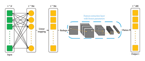
CNN is a feedforward ANN that includes convolutional operations capable of automatically extracting features from data with a convolutional structure. It mainly consists of the convolutional layer, pooling layer, and fully connected layer, where the convolutional layer is responsible for extracting local features from images, and the pooling layer is used to reduce feature dimensions. LeNet, proposed by Yann LeCun et al. [27], is the earliest CNN applied to the recognition of the MINIST handwritten dataset, achieving good performance. The feature extraction layer in LeNet consists of two convolutional layers and two pooling layers. After passing through the first convolutional layer with six convolutional kernels, the output shape is 6 × 28 × 28. After the second layer undergoes downsampling of the pooling layer, the output shape becomes 6 × 14 × 14. Following the third layer’s convolution with 16 kernels, the output shape is 16 × 10 × 10. The output after downsampling in the fourth layer is 16 × 5 × 5. After passing through the feature extraction layer, its output will be flattened into 1 × 400 data and inputted into the subsequent fully connected layer to obtain classification probabilities. The feature extraction layer, through multilevel feature extraction and abstraction, can gradually learn higher-level data representations of input data, thus enhancing the network’s ability to represent complex data. Figure 1 illustrates the feature extraction layer of the LeNet network.

Details are in the caption following the image — **Figure 1**
Open in figure viewer PowerPoint

Feature extraction layer of LeNet.

The application of CNN is limited not only to the field of images but also to the regression prediction domains, such as time series forecasting [28] and medical image detection [29]. In light of this, this paper will utilize the feature extraction layer of LeNet to extract input features. The input features are one-dimensional (1-D) while LeNet expects two-dimensional (2-D) inputs. In order to use the feature extraction information, this paper will map 1-D inputs to 2-D latent variables, thus serving as the input for the CNN.

2.3. Skip Connection

In DL, skip connection refers to bypassing certain layers in the ANN, where the input of these layers is directly added to their output after processing. Skip connection can be used to improve the training and performance of ANN. Due to the increase in depth of deep neural network (DNN), their performance may degrade, leading to the problem of degradation. This could be caused by issues such as vanishing or exploding gradients. To alleviate this problem, residual neural networks [30] first introduced skip connection in DNN, where the input features are directly added to the output features. Therefore, the dimensions of input and output features need to be the same. This design enables the network to more easily learn residuals instead of directly learning low-level features, thereby effectively mitigating the problems of vanishing and exploding gradients in DNN. Skip connections through residual learning make the model easier to optimize and improve prediction accuracy [31]. DenseNet [32] achieves skip connections by concatenating input features with output features, thereby enabling feature reuse and facilitating the flow of information. Khan et al. [33] enhanced feature propagation and utilization in stacked autoencoders through dense connections to address the vanishing gradient problem and improve convergence speed. In light of this, this paper will employ skip connection to achieve feature reusability.

2.4. Transfer Learning

The research on transfer learning originates from an observation that humans can apply previously acquired knowledge to solve new problems, achieving faster or better results. Transfer learning involves learning knowledge or experience from previous tasks and applying it to new tasks. In other words, the purpose of transfer learning is to extract knowledge and experience from one or more source tasks, and then apply it to a target domain.

Transfer learning is a type of ML technique. As the name suggests, it involves transferring the parameters of a pretrained model to a new model to assist in its training. Considering that most data or tasks are correlated, transfer learning allows the sharing of learned model parameters (also understood as knowledge acquired by the model) through some means to accelerate and optimize the learning efficiency of the new model, thus avoiding the need to learn from scratch like most networks [34].

Progressive neural network [35] trains on the source domain (pretrain) and fine-tunes on the target domain to solve problems in the target domain. To prevent forgetting past tasks, the network for each task is preserved after training and the parameters are fixed and no longer updated. When a new task arises, a new network is instantiated. Transfer learning is also applied to the problems where the source domain and target domain are similar, but the target domain has very limited data. Zhang et al. [36] applied transfer learning to few-shot learning problems, demonstrating that a feature extractor learned from the source domain is useful in recognizing novel categories that have only limited data in the target domain. To shorten training time and reduce training costs, this paper uses a transfer learning approach, freezing the feature extraction layer of LeNet and transforming antenna features to a source domain similar to the pretrained LeNet training data for feature extraction.

3. The Proposed Algorithm

3.1. Feature Extraction

In order to use a CNN for feature extraction from 1-D input features, they are first input into a multineuron single-layer perceptron to map the low-dimensional data to a latent variable space. Here, because the input of the pretrained LeNet network is a 28 × 28-dimensional grayscale image, we map the 1-D features to 1 × 784-dimensional latent variable data. The CNN used for feature extraction adopts the method of transfer learning, utilizing the feature extraction layer of the pretrained LeNet network for feature extraction, and freezing the weights and biases of the feature extraction layer to save training costs. To make the input data similar to the source domain of the pretrained network, the data are linearly mapped to the range of 0–255 using formula (8), and then reshaped into a 28 × 28-dimensional grayscale image. After feature extraction, the input features become 16 × 5 × 5-dimensional data, which are flattened into 1 × 400-dimensional data for the input into the BNN for training.

()

where x_max represents the maximum value in the features, x_min represents the minimum value in the features, x represents the feature to be mapped, and x_new represents the mapped latent variable feature. Figure 2 depicts the flowchart of the feature extraction part.

3.2. Feature Fusion

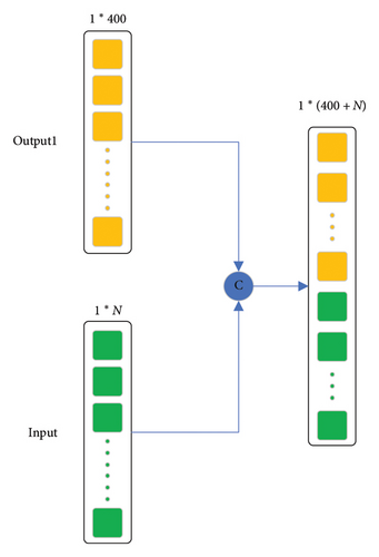
Features extracted by CNN may lose some useful information from the original features. To preserve the problem, a skip connection method is used to fuse the original features with the output features of the CNN.

Since the number of original features is different from the number of extracted features, a concatenation method is chosen to merge the features.

()

where x_fusion represents the fused feature, x_a represents the original feature, and x_b represents the feature extracted through the convolutional layer. Figure 3 illustrates the schematic diagram of concatenating and merging two sets of features.

3.3. The Structure of BNN

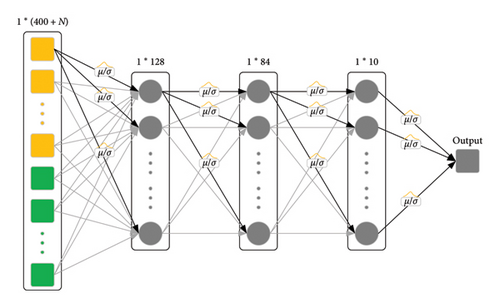
After feature extraction and feature fusion, the new features are used as input to train the BNN. In this study, we freeze the feature extraction layer of the pretrained LeNet network and use it for feature extraction. At the same time, we remove its fully connected layers and replace them with an equivalent BNN structure. During training, only the fully connected layers represented by the BNN are trained. In addition, to mitigate overfitting, dropout algorithm is applied after the second layer of Bayesian linear layer, and early stopping is also used. Using a BNN as the fully connected layers enables the model to have the ability to quantify uncertainty. Model fine-tuning also preserves the excellent feature extraction capability of the convolutional layers of the LeNet network, thus improving the generalization and fitting ability of the BNN. Figure 4 illustrates the structure of the BNN.

3.4. The Proposed Ski-Le-BNN

As already described, the algorithm proposed in this paper consists of three parts: feature extraction, feature fusion, and BNN, named Ski-Le-BNN. The original features are first processed and transformed into 2-D latent variables, which are input into a feature extraction layer with frozen weights for extracting the features. Subsequently, the output is concatenated with the original features to achieve feature reusability. The concatenated features are then used as input to train the BNN, ultimately resulting in obtaining well-trained model parameters. The pseudocode of the proposed algorithm is shown in Algorithm 1.

Algorithm 1: Model Training Process for Ski-Le-BNN.

Input: Data set [x, y]
Output: model parameters
1.
Employ a single-layer perceptron with multiple neurons to map the original feature vector x to the latent variable space x’;
2.
Linearly map x’ to the range of 0–255 using Equation (8);
3.
Convert it into a 2-D grayscale image to obtain x’’;
4.
Instantiate the LeNet model, load pretrained parameters, and remove the fully connected layer;
5.
Pass x’’ through the feature extraction layer with frozen weights to obtain output 1;
6.
Fuse output 1 with the original features to obtain new features x^∗ according to Equation (9);
7.
for epoch in epochs do
8.
Train BNN using [x^∗, y];
9.
if meet the stop conditions then
10.
Save network model;
11.
break;
12.
end if
13.
end for

4. Experimental Results

4.1. Model Performance Metrics

This paper selects mean square error (MSE), mean absolute error (MAE), and R-square (R²) as the evaluation metrics for model performance. MSE and MAE are commonly used evaluation metrics for regression models. MSE measures the average of the squared differences between the predicted values and the true values, while MAE measures the average of the absolute error. R² is a statistical measure used to assess the fitness of a regression model. It represents the proportion of the variance in the dependent variable that is predictable from the independent variables.

()

where m represents the sample size, y_i denotes the true value of the i_th observation,

represents the model’s predicted value for the i_th observation, and

denotes the mean value of all observations.

4.2. Antenna Modeling and Results Analysis

4.2.1. Symmetric Coplanar Waveguide (CPW) Fed Patch Antenna

A symmetric CPW-fed patch antenna designed for WLAN and WiMAX is as an example to validate the proposed model’s effectiveness. The antenna operates in the frequency range of 2 through 6.5 GHz. The S₁₁ parameters of the antenna are modeled using the method proposed in this paper, and the dataset is obtained through full-wave EM simulation software HFSS. The antenna structure, as shown in Figure 5, is printed on an FR4 dielectric substrate with a thickness of 1.56 mm. The relative dielectric constant of the substrate is 4.3, and the dielectric loss tangent is 0.020. The patch is composed of a circular conductor with a radius of 10.5 mm and a metal thickness of 0.035 mm. The antenna dimensions are 24 × 33.5 × 1.56 mm³, offering the advantages of small size and simple structure. The CPW transmission line used to feed the antenna consists of a signal strip with a width of 3.2 mm and a gap distance of 0.5 mm between the signal strip and the coplanar ground plane. The feeding impedance of the antenna is 50 Ω.

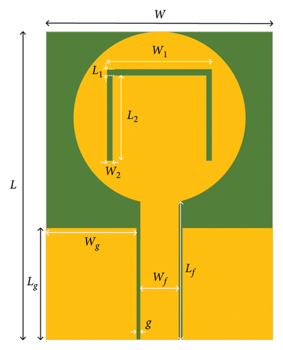
To confine the antenna radiation within the desired resonance frequency range, a C-shaped slot is etched on the circular patch, consisting of three rectangles with parameters L1, W1, L2, and W2. We select P = [L1, W1, L2, W2] as the varying parameters for the antenna modeling. Table 1 shows the variation range of the selected physical parameters.

Table 1. Varying parameters of the CPW-fed patch antenna.

Varying parameters	Data range (mm)
L1	0.6–1.05
W1	11.5–13.5
L2	10.5–12.5
W2	0.45–∼0.9

Firstly, 100 sets of antenna samples are selected using the latin hypercube sampling method. Then, Python is used to call HFSS to simulate the antenna sample set, obtaining the S₁₁ parameters of each sample within the frequency range of 2 through 6.5 GHz. To fully simulate the variation trend of the antenna within the operating frequency range, the sweep step is set to 0.05 GHz, thereby generating 91 sampling points representing the change of S₁₁ parameters across the entire frequency band. Each EM simulation costs about 48 s on average. The dataset was divided with 80% as the training set and 20% as the testing set. This division method aims to ensure that the model has sufficient samples to learn the underlying features during the training process while retaining a certain proportion of the data for subsequent performance evaluation.

Table 2 presents the comparison of S₁₁ prediction performance for the patch antenna using different modeling algorithms. In this paper, all models are trained on a workstation equipped with an Intel(R) Core (TM) i9-10900X CPU (3.7 GHz) and NVIDIA GeForce RTX 3090. The Le-BNN model combines the feature extraction method proposed in this paper with BNN, without using feature fusion. From Table 2, it can be observed that the R² of Le-BNN has improved by 11.9% compared to the standalone BNN, while MSE has decreased by 52.4% and MAE has decreased by 38.5%. Furthermore, with the addition of skip connections in the model, the performance is further improved. R² has increased by 1.28% compared to Le-BNN, while MSE has decreased by 13.3% and MAE has decreased by 10.5%. It can also be observed that the improvement of Le-BNN over BNN is greater than that of Ski-Le-BNN over Le-BNN. However, Ski-Le-BNN performs the best among the three models. This is because the convolutional layers of LeNet can effectively extract spatial features after feature fusion, enhancing the model’s generalization ability. However, because of the loss of some useful original features after feature fusion, its performance is weaker than that of the ski-Le-BNN with skip connections. The model proposed in this study outperforms the two comparison models in terms of MSE, MAE, and R² performance indicators. In addition, Le-BNN also outperforms the BNN model in all performance metrics. The Ski-Le-BNN model training time is 570 s. Thus, significant improvement in model performance and the effectiveness of the model for antenna modeling are evident from the innovative points proposed in this paper.

Table 2. Performance comparison of different modeling methods for the CPW-fed patch antenna.

Models	MSE	MAE	R²
BNN	4.4438	1.3442	0.8146
Le-BNN	2.1140	0.8262	0.9116
Proposed Ski-Le-BNN	1.8335	0.7393	0.9233

Table 3 presents the performance metrics of different models for the CPW-fed, dual-band patch antenna. In this study, the ANN employs a two-layer hidden structure, with the first layer consisting of 32 neurons and the second layer consisting of 64 neurons, utilizing MSE as the loss function. For the antenna dataset, the LeNet model adds an additional fully connected layer based on the introduction in the relevant technical section, enabling the mapping of antenna features to a high-dimensional space. The remaining models are trained using the default settings provided by Scikit-learn. As shown in Table 3, the model proposed in this paper demonstrates superior performance across all metrics compared to other benchmark models.

Table 3. Performance metrics of different modeling models for the CPW-fed patch antenna.

Models	MSE	MAE	R²
Artificial neural network	3.2511	1.0160	0.8538
K-nearest neighbors	7.4321	1.4235	0.6920
LeNet	5.8684	1.4718	0.7568
Decision tree	10.8292	1.5883	0.5513
Random forest	4.6623	1.1338	0.8068
Proposed Ski-Le-BNN	1.8335	0.7393	0.9233

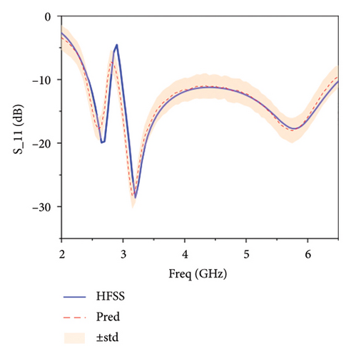
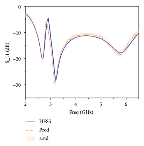
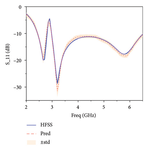
Figure 6 illustrates the comparison between the predictions and the actual values of the same antenna parameters by different models. From Figure 6(a), it can be observed that the BNN exhibits the biggest deviation from the actual values, and the prediction uncertainty is also the highest, which indicates that the model’s performance in antenna modeling has not yet reached its optimum. In Figure 6(b), it is evident that Le-BNN shows a significant improvement in fitting to the actual values compared to BNN, and the prediction uncertainty has also decreased significantly. However, it is still weaker than the fitting capability of the model proposed in this paper, as shown in Figure 6(c).

4.2.2. Double T-Shaped Monopole Antenna

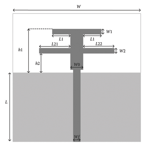
The second example is a double T-shaped monopole antenna, which combines two T-shaped structures with different sizes, enabling the antenna to operate within the WLAN communication frequency band. The antenna is shown in Figure 7, with the substrate material being FR4, thickness of 0.8 mm, relative dielectric constant of 4.4, and feed impedance of 50 Ω. The fixed physical parameters of the antenna are shown in Table 4.

Table 4. Fixed parameters of the double T-shaped monopole antenna.

Parameters	Fixed value (mm)
L	50
W	75
h1	14.5
h2	2
L1	5.3
Wf	1.5

The S₁₁ parameter of the antenna mainly depends on five parameters, including L21, L22, W0, W1, and W2. Therefore, we select the five parameters as variables to construct the antenna dataset, and their ranges are shown in Table 5. Similarly, using the Latin hypercube sampling method, we obtain a dataset of 100 samples, and simulate their S₁₁ parameter using HFSS from 1.5 to 6 GHz. The sampling step is set to 0.01 GHz. Each EM simulation costs about 70 s on average.

Table 5. Varying parameters of the double T-shaped monopole antenna.

Varying parameters	Data range (mm)
L21	6.3–7.3
L22	6.3–7.3
W0	1.5–3.5
W1	1.5–2.5
W2	1.5–2.5

Table 6 shows the comparison of S₁₁ prediction performance for the double T-shaped monopole antenna using different algorithms. From Table 6, it can be observed that the R² of Le-BNN is 5.6% higher than that of BNN, with a 43.6% decrease in MSE and a 10.2% decrease in MAE. Similarly, the performance of Ski-Le-BNN shows further improvement compared to Le-BNN, with an increase of 1.5% in R², a decrease of 22.7% in MSE, and a decrease of 3.9% in MAE. Among the three prediction performance metrics in Table 6, the Ski-Le-BNN performs the best, followed by the Le-BNN, with the standalone BNN performing the worst. The Ski-Le-BNN model training time is 880 s. This conclusion is consistent with the results in Example 1, indicating the effectiveness of the proposed structure in enhancing the modeling performance of the BNN antenna.

Table 6. Performance comparison of different modeling methods for the double T-shaped monopole antenna.

	MSE	MAE	R²
BNN	0.6281	0.4346	0.8880
Le-BNN	0.3540	0.3904	0.9373
Proposed Ski-Le-BNN	0.2736	0.3753	0.9512

Table 7 presents the performance metrics of different models for the double T-shaped monopole antenna, with the compared models being consistent with those in Table 3. According to the results in Table 7, the surrogate model proposed in this paper still outperforms other models across all performance metrics. This result indicates that the proposed model maintains exceptional performance across different antenna structures, further validating its applicability and generalization capability.

Table 7. Performance metrics of different modeling models for the double T-shaped monopole antenna.

Models	MSE	MAE	R²
Artificial neural network	0.9660	0.4463	0.8389
K-nearest neighbors	0.3761	0.4270	0.9330
LeNet	0.3766	0.4714	0.9329
Decision tree	0.5480	0.4547	0.9023
Random forest	0.2894	0.3758	0.9484
Proposed Ski-Le-BNN	0.2736	0.3753	0.9512

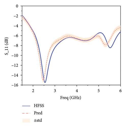
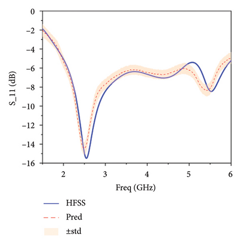
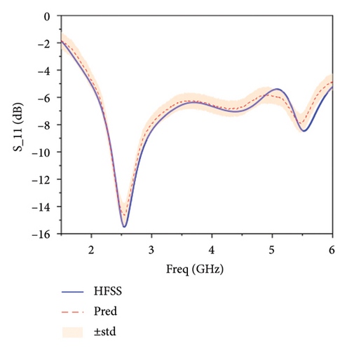
Figure 8 illustrates the comparison between the predicted values and the actual values by different models. Figure 8(a) shows the predicted S₁₁ parameter by the standalone BNN, indicating a general trend of the antenna’s S₁₁ parameter but with deviations. Figure 8(b) presents the S₁₁ parameter predicted by the Le-BNN, showing a closer approximation to the real values compared to the standalone BNN. In Figure 8(c), the prediction using the Ski-Le-BNN is the closest to the real values among the three models. Therefore, the Ski-Le-BNN model proposed in this paper demonstrates the best fitting performance, followed by the Le-BNN, with the standalone BNN performing the worst. This highlights the effectiveness of the proposed model for antenna modeling.

5. Conclusion

This study combines the advantages of CNN in spatial feature extraction and the feature reusability of skip connections exploiting the statistically based prediction uncertainty of BNN, and proposes the Ski-Le-BNN modeling method. The effectiveness of the method is validated through two antenna examples, including a symmetric CPW-fed patch antenna and a double T-shaped monopole antenna. From the experiment results, the performance of the proposed method is superior to that of the BNN, greatly improving the fitting performance and generalization ability of the BNN for antenna modeling. Therefore, for data-driven antenna optimization problems, the proposed ski-Le-BNN can serve as a surrogate model. Future work will focus on extending the proposed method to more complex design variables for modeling various types of antennas. Furthermore, in addition to predicting S-parameters, future research will also explore the prediction of other key electrical performance metrics, such as gain, radiation efficiency, and directivity.

Conflicts of Interest

The authors declare no conflicts of interest.

Author Contributions

Yubo Tian and Jinlong Sun are co-first authors, with Yubo Tian serving as the corresponding author.

Funding

This work was supported by the Natural Science Foundation of Guangdong Province of China under Grant No. 2023A1515011272, the Tertiary Education Scientific research project of Guangzhou Municipal Education Bureau of China under No. 202234598, the Special Project in Key Fields of Guangdong Universities of China under No. 2022ZDZX1020, and the Scientific Research Capacity Improvement Project of Key Developing Disciplines in Guangdong Province of China under No. 2021ZDJS057.

Acknowledgments

This work was supported by the Natural Science Foundation of Guangdong Province of China under Grant No. 2023A1515011272, the Tertiary Education Scientific research project of Guangzhou Municipal Education Bureau of China under No. 202234598, the special project in key fields of Guangdong Universities of China under No. 2022ZDZX1020, and the scientific research capacity improvement project of key developing disciplines in Guangdong Province of China under No.2021ZDJS057.

Open Research

Data Availability Statement

The data that support the findings of this study are available from the corresponding author upon reasonable request.

References

1 Rocca P., Oliveri G., and Massa A., Differential Evolution as Applied to Electromagnetics, IEEE Antennas and Propagation Magazine. (2011) 53, no. 1, 38–49, https://doi.org/10.1109/map.2011.5773566, 2-s2.0-79960489798.
10.1109/MAP.2011.5773566
Web of Science® Google Scholar
2 Sato Y., Campelo F., and Igarashi H., Meander Line Antenna Design Using an Adaptive Genetic Algorithm, IEEE Transactions on Magnetics. (2013) 49, no. 5, 1889–1892, https://doi.org/10.1109/tmag.2013.2239979, 2-s2.0-84877851563.
10.1109/TMAG.2013.2239979
Web of Science® Google Scholar
3 Koziel S. and Ogurtsov S., Antenna Design by Simulation-Driven Optimization, SpringerBriefs in Optimization, 2014, Springer International Publishing, Cham.
Google Scholar
4 Hassan A.-K. S. O., Etman A. S., and Soliman E. A., Optimization of a Novel Nano Antenna with Two Radiation Modes Using Kriging Surrogate Models, IEEE Photonics Journal. (2018) 10, no. 4, 1–17, https://doi.org/10.1109/jphot.2018.2848593, 2-s2.0-85048602330.
10.1109/JPHOT.2018.2848593
Web of Science® Google Scholar
5 Sun C., Jin Y., Cheng R., Ding J., and Zeng J., Surrogate-Assisted Cooperative Swarm Optimization of High-Dimensional Expensive Problems, IEEE Transactions on Evolutionary Computation. (2017) 21, no. 4, 644–660, https://doi.org/10.1109/tevc.2017.2675628, 2-s2.0-85026880187.
10.1109/TEVC.2017.2675628
Web of Science® Google Scholar
6 Liu B., Aliakbarian H., Ma Z., Vandenbosch G. A. E., Gielen G., and Excell P., An Efficient Method for Antenna Design Optimization Based on Evolutionary Computation and Machine Learning Techniques, IEEE Transactions on Antennas and Propagation. (2014) 62, no. 1, 7–18, https://doi.org/10.1109/tap.2013.2283605, 2-s2.0-84892405285.
10.1109/TAP.2013.2283605
Web of Science® Google Scholar
7 Xiao L.-Y., Shao W., Jin F.-L., and Wang B.-Z., Multiparameter Modeling with ANN for Antenna Design, IEEE Transactions on Antennas and Propagation. (2018) 66, no. 7, 3718–3723, https://doi.org/10.1109/tap.2018.2823775, 2-s2.0-85045207220.
10.1109/TAP.2018.2823775
Web of Science® Google Scholar
8 Jin Y., Olhofer M., and Sendhoff B., A Framework for Evolutionary Optimization with Approximate Fitness Functions, IEEE Transactions on Evolutionary Computation. (2002) 6, no. 5, 481–494, https://doi.org/10.1109/tevc.2002.800884, 2-s2.0-0036808455.
10.1109/TEVC.2002.800884
Web of Science® Google Scholar
9 Luo Y., Duan S., Ning Chen Z., Yan N., An W., and Ma K., An Artificial-Neural-Network-Based Efficient Beamforming Synthesis Method and its Application to Flat-Top Beamformed Compressed High-Order-Mode Dipoles, IEEE Transactions on Antennas and Propagation. (2024) 72, no. 10, 7606–7614, https://doi.org/10.1109/tap.2024.3450304.
10.1109/TAP.2024.3450304
Google Scholar
10 Ren X., Tian Y., Li Q., and Fu H., Resonant Frequency Modelling of Microstrip Antennas by Consensus Network and Student’s T Process, Applied Computational Electromagnetics Society Journal. (2024) 38, no. 12, 987–997, https://doi.org/10.13052/2023.aces.j.381209.
10.13052/2023.aces.j.381209
Google Scholar
11 Chavez-Hurtado J. L. and Rayas-Sanchez J. E., Polynomial-Based Surrogate Modeling of RF and Microwave Circuits in Frequency Domain Exploiting the Multinomial Theorem, IEEE Transactions on Microwave Theory and Techniques. (2016) 64, no. 12, 4371–4381, https://doi.org/10.1109/tmtt.2016.2623902, 2-s2.0-84996928627.
10.1109/TMTT.2016.2623902
Web of Science® Google Scholar
12 Prado D. R., Lopez-Fernandez J. A., Arrebola M., and Goussetis G., Support Vector Regression to Accelerate Design and Crosspolar Optimization of Shaped-Beam Reflectarray Antennas for Space Applications, IEEE Transactions on Antennas and Propagation. (2019) 67, no. 3, 1659–1668, https://doi.org/10.1109/tap.2018.2889029, 2-s2.0-85058999653.
10.1109/TAP.2018.2889029
Web of Science® Google Scholar
13 Contal E., Buffoni D., Robicquet A., and Vayatis N., H. Blockeel, K. Kersting, S. Nijssen, and F. Železný, Parallel Gaussian Process Optimization with Upper Confidence Bound and Pure Exploration, Machine Learning and Knowledge Discovery in Databases, 2013, Springer, Berlin, Heidelberg, 225–240.
Google Scholar
14 Hua Q., Huang Y., Song C. et al., A Novel Compact Quadruple-Band Indoor Base Station Antenna for 2G/3G/4G/5G Systems, IEEE Access. (2019) 7, 151350–151358, https://doi.org/10.1109/access.2019.2947778.
10.1109/ACCESS.2019.2947778
Google Scholar
15 Blundell C., Cornebise J., Kavukcuoglu K., and Wierstra D., Weight Uncertainty in Neural Networks, 2015.
Google Scholar
16 Liu Y., Liu B., Ur-Rehman M. et al., An Efficient Method for Antenna Design Based on a Self-Adaptive Bayesian Neural Network-Assisted Global Optimization Technique, IEEE Transactions on Antennas and Propagation. (Dec. 2022) 70, no. 12, 11375–11388, https://doi.org/10.1109/tap.2022.3211732.
10.1109/TAP.2022.3211732
Google Scholar
17 Simon S., Schwarz G. M., Aichmair A., Frank B. J., Hummer A., DiFranco M. D., Dominkus M., and Hofstaetter J. G., Fully Automated Deep Learning for Knee Alignment Assessment in Lower Extremity Radiographs: a Cross-Sectional Diagnostic Study, Skeletal Radiology. (2022) 51, no. 6, 1249–1259, https://doi.org/10.1007/s00256-021-03948-9.
10.1007/s00256-021-03948-9
PubMed Google Scholar
18 Calik N., Güneş F., Koziel S., Pietrenko-Dabrowska A., Belen M. A., and Mahouti P., Deep-learning-based Precise Characterization of Microwave Transistors Using Fully-Automated Regression Surrogates, Scientific Reports. (2023) 13, no. 1, https://doi.org/10.1038/s41598-023-28639-4.
10.1038/s41598-023-28639-4
Web of Science® Google Scholar
19 Sun K. and Tian Y., DBFNet: A Dual-Branch Fusion Network for Underwater Image Enhancement, Remote Sensing. (2023) 15, no. 5, https://doi.org/10.3390/rs15051195.
10.3390/rs15051195
Google Scholar
20 Fu H., Tian Y., Meng F., Li Q., and Ren X., Microstrip Antenna Modelling Based on Image-Based Convolutional Neural Network, Electronics Letters. (2023) 59, no. 16, https://doi.org/10.1049/ell2.12910.
10.1049/ell2.12910
Google Scholar
21 Zhu Z., Tian Y., and Sun J., Antenna Modeling Based on Image-CNN-LSTM, IEEE Antennas and Wireless Propagation Letters. (2024) 23, no. 9, 2738–2742, https://doi.org/10.1109/lawp.2024.3405996.
10.1109/LAWP.2024.3405996
Google Scholar
22 Wei Z., Zhou Z., Wang P. et al., Fast and Automatic Parametric Model Construction of Antenna Structures Using CNN–LSTM Networks, IEEE Transactions on Antennas and Propagation. (2024) 72, no. 2, 1319–1328, https://doi.org/10.1109/tap.2023.3346050.
10.1109/TAP.2023.3346050
Google Scholar
23 Ding W.-T., Meng F., Tian Y.-B., and Yuan H.-N., Antenna Optimization Based on Auto-Context Broad Learning System, International Journal of Antennas and Propagation. (2022) 2022, 1–10, https://doi.org/10.1155/2022/7338164.
10.1155/2022/7338164
Web of Science® Google Scholar
24 Wang H. and Yeung D.-Y., Towards Bayesian Deep Learning: A Framework and Some Existing Methods, IEEE Transactions on Knowledge and Data Engineering. (Dec. 2016) 28, no. 12, 3395–3408, https://doi.org/10.1109/tkde.2016.2606428, 2-s2.0-85027053369.
10.1109/TKDE.2016.2606428
Web of Science® Google Scholar
25 Sun Z., Research on Low Overhead Bayesian Neural Network Inference Accelerator, 2022, University of Electronic Science and technology.
Google Scholar
26 Aliqab K., Sohaib M. A., Ali F., Armghan A., and Alsharari M., Employment of Self-Adaptive Bayesian Neural Network for Systematic Antenna Design: Improving Wireless Networks Functionalities, Micromachines. (2023) 14, no. 3, https://doi.org/10.3390/mi14030594.
10.3390/mi14030594
Google Scholar
27 Lecun Y., Bottou L., Bengio Y., and Haffner P., Gradient-based Learning Applied to Document Recognition, Proceedings of the IEEE. (1998) 86, no. 11, 2278–2324, https://doi.org/10.1109/5.726791, 2-s2.0-0032203257.
10.1109/5.726791
Web of Science® Google Scholar
28 Durairaj D. M. and Mohan B. H. K., A Convolutional Neural Network Based Approach to Financial Time Series Prediction, Neural Computing & Applications. (2022) 34, no. 16, 13319–13337, https://doi.org/10.1007/s00521-022-07143-2.
10.1007/s00521-022-07143-2
PubMed Web of Science® Google Scholar
29 Ganokratanaa T., Ketcham M., and Pramkeaw P., Advancements in Cataract Detection: The Systematic Development of LeNet-Convolutional Neural Network Models, Journal of Imaging. (2023) 9, no. 10, https://doi.org/10.3390/jimaging9100197.
10.3390/jimaging9100197
PubMed Google Scholar
30 He K., Zhang X., Ren S., and Sun J., Deep Residual Learning for Image Recognition, 2015.
Google Scholar
31 Xu G., Wang X., Wu X., Leng X., and Xu Y., Development of Skip Connection in Deep Neural Networks for Computer Vision and Medical Image Analysis: A Survey, 2024.
Google Scholar
32 Huang G., Liu Z., van der Maaten L., and Weinberger K. Q., Densely Connected Convolutional Networks, arXiv, Jan. 28. (2018) .
Google Scholar
33 Khan Z. A., Hussain T., Ullah F. U. M., Gupta S. K., Lee M. Y., and Baik S. W., Randomly Initialized CNN with Densely Connected Stacked Autoencoder for Efficient Fire Detection, Engineering Applications of Artificial Intelligence. (2022) 116, https://doi.org/10.1016/j.engappai.2022.105403.
10.1016/j.engappai.2022.105403
Google Scholar
34 Iman M., Arabnia H. R., and Rasheed K., A Review of Deep Transfer Learning and Recent Advancements, Technologies. (2023) 11, no. 2, https://doi.org/10.3390/technologies11020040.
10.3390/technologies11020040
Web of Science® Google Scholar
35 Rusu A. A., Progressive Neural Networks, arXiv. (2022) .
Google Scholar
36 Das D. and George Lee C. S., Zero-shot Image Recognition Using Relational Matching, Adaptation and Calibration, 2019 International Joint Conference on Neural Networks (IJCNN). (2019) 1–8, https://doi.org/10.1109/ijcnn.2019.8852315, 2-s2.0-85073227298.
10.1109/ijcnn.2019.8852315
Google Scholar

All articles

Skip-Connected CNN Exploiting BNN Surrogate for Antenna Modelling

Abstract

1. Introduction

2. Related Works

2.1. BNN

2.2. CNN

2.3. Skip Connection

2.4. Transfer Learning

3. The Proposed Algorithm

3.1. Feature Extraction

3.2. Feature Fusion

3.3. The Structure of BNN

3.4. The Proposed Ski-Le-BNN

4. Experimental Results

4.1. Model Performance Metrics

4.2. Antenna Modeling and Results Analysis

4.2.1. Symmetric Coplanar Waveguide (CPW) Fed Patch Antenna

4.2.2. Double T-Shaped Monopole Antenna

5. Conclusion

Conflicts of Interest

Author Contributions

Funding

Acknowledgments

Open Research

Data Availability Statement

References

Figures

References

Information

About Wiley Online Library

Help & Support

Opportunities

Connect with Wiley