International Journal of Aerospace Engineering

Volume 2025, Issue 1 4107637

Research Article

Open Access

Fuzzy Consensus Cubature Information Filtering for Space Target Tracking

Xiaobo Zhang,

Xiaobo Zhang

orcid.org/0000-0003-2340-158X

Department of Electronic Engineering , PLA Rocket Force University of Engineering , Xi’an , Shaanxi , China

Search for more papers by this author

Bing He,

Corresponding Author

Bing He

[email protected]

orcid.org/0009-0005-6792-8385

Department of Electronic Engineering , PLA Rocket Force University of Engineering , Xi’an , Shaanxi , China

Search for more papers by this author

Gang Liu,

Gang Liu

Department of Electronic Engineering , PLA Rocket Force University of Engineering , Xi’an , Shaanxi , China

Search for more papers by this author

Haoshen Lin,

Haoshen Lin

Department of Electronic Engineering , PLA Rocket Force University of Engineering , Xi’an , Shaanxi , China

Search for more papers by this author

Zifeng Gong,

Zifeng Gong

Department of Electronic Engineering , PLA Rocket Force University of Engineering , Xi’an , Shaanxi , China

Search for more papers by this author

Xiaobo Zhang,

Xiaobo Zhang

orcid.org/0000-0003-2340-158X

Department of Electronic Engineering , PLA Rocket Force University of Engineering , Xi’an , Shaanxi , China

Search for more papers by this author

Bing He,

Corresponding Author

Bing He

[email protected]

orcid.org/0009-0005-6792-8385

Department of Electronic Engineering , PLA Rocket Force University of Engineering , Xi’an , Shaanxi , China

Search for more papers by this author

Gang Liu,

Gang Liu

Department of Electronic Engineering , PLA Rocket Force University of Engineering , Xi’an , Shaanxi , China

Search for more papers by this author

Haoshen Lin,

Haoshen Lin

Department of Electronic Engineering , PLA Rocket Force University of Engineering , Xi’an , Shaanxi , China

Search for more papers by this author

Zifeng Gong,

Zifeng Gong

Department of Electronic Engineering , PLA Rocket Force University of Engineering , Xi’an , Shaanxi , China

Search for more papers by this author

First published: 06 June 2025

https://doi.org/10.1155/ijae/4107637

Academic Editor: Giovanni Palmerini

Share a link

Email
Wechat
Bluesky

Abstract

A fuzzy distributed nonlinear state estimation issue on the possibilistic framework is investigated in this paper. Firstly, unlike the Gaussian probability distributions on the traditional probability framework, the noises are modeled as fuzzy random variables (FRVs) with trapezoidal possibility distributions (TPDs), and then a fuzzy cubature paradigm is proposed. Secondly, based on the fuzzy cubature paradigm, a novel fuzzy consensus cubature information filtering (FCCIF) algorithm is proposed for sensor networks wherein each agent fuses local fuzzy information with fuzzy information from the neighbors based on the weighted average consensus. Furthermore, under well-known observability and connectivity assumptions, it is proved that the FCCIF possesses guaranteed stability regardless of consensus steps. Finally, a space target tracking simulation is developed to verify the validity of the FCCIF algorithm. The FCCIF algorithm can be used in navigation guidance, radar tracking, sonar ranging, satellite orbit determination, and other practical applications when the noises are suitable for qualitative rather than quantitative description.

1. Introduction

In recent years, space situational awareness (SSA) has attracted extensive attention from various countries [1–3]. Space target tracking is a basic work because other space tasks are based on it [4, 5]. Due to the ability of real-time estimation and nonstationary process tracking [6, 7], the Kalman filter is widely used in space target tracking, which is essentially a nonlinear state estimation issue. The extended Kalman filter (EKF) is a widely used prediction method due to it being simple and easy to understand [8]. However, its Jacobian matrix is difficult to calculate, and it may diverge when ignoring the Taylor expansion terms. The unscented Kalman filter (UKF) algorithm was a sampling filter utilizing the unscented transformation [9]. A key drawback of the UKF is that the calculation of the covariance matrix may be negatively definite. To overcome this limitation, the cubature Kalman filter (CKF) and the square root cubature Kalman filter (SRCKF) were proposed [10, 11].

Due to the limited sensing and computing ability, it is difficult for a single sensor to complete the target track and control task [12]. With the rapid development of sensor networks, distributed filtering and control are widely studied in many existing works. Considering the complex space environment, Jia et al. [13] presents a consensus cubature information filtering (CCIF) algorithm for space target tracking, which can achieve satisfactory results. Hu et al. [14] introduced a Kullback–Leibler divergence-based consensus cubature Kalman filter (CCKF), which can solve the problems of switching topology and different space target sensors with different observation equations. To take advantage of joint tracking, Chen et al. [15] proposed a composite weighted average consensus filter, in which the ground-based radar used a sparse-grid quadrature filter (SGQF) while the space optical sensor (SOS) used an EKF. To use sensors with different sampling times and different sampling rates for collaborative tracking, Hu et al. [16] presented a universal consensus filter (UCF). Jia et al. [17] proposed a diffusion-based enhanced covariance intersection cooperative space target tracking (DECISPOT) filter, which can improve track accuracy when measurements do not exist or are of low accuracy. Zhang et al. [18] studied a distributed strong tracking filter algorithm to resist maneuver uncertainty. Zhou et al. [19] proposed a distributed multiple-model nonlinearity filter for tracking the highly mobile noncooperative targets. Doostmohammadian et al. [20] proposed a distributed estimation approach requiring less networking and communication traffic and was applied to track a mobile target via the formation of unmanned aerial vehicles.

Notably, the event definitions of the abovementioned filtering algorithms are all clear, and the progress and observer noises are assumed to obey a Gaussian distribution. However, in some scenarios, there exists uncertainty [20] and noises that do not obey a Gaussian distribution. For example, because of the space environment, a quantitative description of the relationship between noise and environment is too complicated to be used, so that noise must be quantitatively described with fuzziness [21]. Moreover, due to the drift of the sensor, the measurement results have great uncertainty and a bit of distrust; thus, the measurement noise may not exhibit a Gaussian distribution [21]. Furthermore, for noncooperative targets, the noises have high uncertainty as they often depend on the experience of experts. In these scenarios, the precise, quantitative, and probabilistic Kalman filter is difficult to meet the application requirements [22].

When in face of these scenarios, researchers proposed a multifarious fuzzy Kalman filter (FKF) by combining fuzzy logic [23–25] with the Kalman filter. FKF uses fuzzy logic to express uncertainty so that precise mathematical models are not needed to deal with complex problems. Yan et al. [26] proposed a fuzzy adaptive strong tracking filter, in which the Takagi–Sugeno (T–S) model is used for fuzzy reasoning for GPS navigation. Jwo and Wang [27] proposed a robust adaptive filter using fuzzy logic for a tightly coupled visual-inertial odometry navigation system. Yue et al. [28] proposed an INS/GPS sensor fusion algorithm based on adaptive fuzzy EKF with sensitivity to disturbances. Sabzevari and Chatraei [29] introduced fuzzy random variables (FRVs) with trapezoidal possibility distributions (TPDs) and proposed a novel fuzzy extended Kalman filter (FEKF) for robot localization. Mata et al. [30] proposed a fuzzy square root cubature Kalman filter (FSRCKF) using FRVs to model noises for spatial target localization. Especially for distributed target tracking, Ye et al. [31] proposed a distributed fuzzy information filtering (DFIF) for linear systems, and Lin et al. [32] proposed a distributed FKF under switching topology for linear systems.

However, a fuzzy distributed Kalman filter suitable for space target tracking needs to be studied. A lot of space target tracking researches are based on assumptions that the noises distributed as probability distributions. In practice, there exist a lot of space target with fuzzy uncertainty in which the noises suit to be modeled as FRVs. For example, if noise does not follow a “bell curve” shape, or is unbalanced, or even we feel a bit of distrust on the value obtained subjectively, we can use a possible region to cover the changing characteristics of the noise. Moreover, according to the available information about noises, the noises in some space target measure systems are better suited to being modeled as FRVs rather than random variables (RVs). For example, a radar sensor with an accuracy of ±2 mm, we have some confidence regarding the distribution of the interval values within the system. It is worth noting that the above FKFs are either suitable for the single-sensor case or the linear case, and a fuzzy distributed Kalman filter suit for strong nonlinear state estimation problems has not been fully studied as far as the authors know. Therefore, this study contributes to expanding research results on [29–32] to strong nonlinear state estimation problems. The noises are modeled as FRVs with TPDs so that a fuzzy cubature paradigm can be proposed. Each agent performs a fuzzy cubature paradigm locally and fuses local fuzzy information with fuzzy information from the neighbors based on the weighted average consensus so that a novel fuzzy consensus cubature information filtering (FCCIF) algorithm is proposed. Compared to the FEKF algorithm and the FSRCK algorithm, which only considered the single-sensor case and were not suitable for the distributed network, the FCCIF algorithm in this paper does not rely on a central node to fully obtain global information and can approach the global posterior estimation only by communicating with neighbors. Compared to the algorithm in [31, 32], which considered linear systems, the FCCIF algorithm in this paper suits for strongly nonlinear systems. Furthermore, the mean square estimation errors of position (MSEP) and the mean square estimation errors of velocity (MSEV) of the FCCIF algorithm are 23% and 90% of the fuzzy consensus extended information filtering (FCEIF), which can be obtained by combining the DFIF in [31] and the EKF. The contributions of this research can be summarized as follows: (1) A fuzzy cubature paradigm is proposed by combining the cubature paradigm and the fuzzy filtering to deal with the strong nonlinear state estimation problems with fuzzy noises. (2) A novel FCCIF algorithm is developed by embedding the fuzzy cubature paradigm into the weighted average consensus frame. (3) The stability of the FCCIF algorithm is investigated.

The article is organized as follows. Section 2 presents preliminary information regarding the TPD and graph theory, along with the problem formulation. Section 3 describes the FCCIF for nonlinear systems. Section 4 investigates the stability of the FCCIF algorithm. Section 5 presents the details of the space target tracking simulations. Section 6 presents the concluding remarks.

1.1. Notations

All vectors are denoted by bold lowercase letters. All matrices are denoted by bold uppercase letters. X(∗)^T, (∗)^TYX, and XY(∗)^T represent XX^T, X^TYX, and XYX^T, respectively. ℝⁿ represents the n-dimensional Euclidean space. ℤ⁺ represents the set of positive integers. Superscript {·}^(l) represents the vertexes of a TPD. {·}^T and {·}⁻¹ represent the transpose operator and the inverse operator, respectively.

2. Preliminaries and Problem Formulation

We first give the preliminary knowledge of graph theory, FRVs, and TPDs; then extract the fuzzy filtering problem; and finally summarize the main targets of this paper.

2.1. Preliminaries

Consider a network consisting of N nodes. An undirected graph describes the communication between sensors, where respect nodes and edges. The set represents the neighbors of node i. represents the inclusive neighborhood of node i. Let with elements a_ij respects the adjacent matrix of graph . Let a_ij > 0 if sensor i and j can exchange information, otherwise a_ij = 0.

Zhang et al. [33] introduced possibility theory, which was established to handle certain types of uncertainty in the first place. A possibility distribution π is a mapping from Ω to [0, 1]. The value π_Ω(x) is defined as the possibility degree of the value x in Ω. Suppose an FRV x defined by a TPD Π(x⁽¹⁾; x⁽²⁾; x⁽³⁾; x⁽⁴⁾) as Figure 1, in which the possibility degree is given as

()

then, the expectation of x is defined as

()

then, the area, center of gravity, and uncertainty of the TPD are given as follows [31]:

()

Details are in the caption following the image — **Figure 1**
Open in figure viewer PowerPoint

Trapezoidal possibility distribution.

is a high-dimensional variable, the distribution of each element is a TPD, that is,

, then, the center of gravity and uncertainty of x are defined as follows [31]:

()

2.2. Problem Formulation

The fuzzy distributed nonlinear estimation problem over the sensor network can be stated as follows. Take into account a discrete-time nonlinear dynamical system.

()

where x_k ∈ ℝⁿ is the target state at time k. State x_k is measured by N sensors in a network, and the estimated mapping of sensor i is

()

where

is the observed value obtained by sensor i. The prior and posterior estimate set of x_k by agent i are denoted as

and

, respectively.

is uncertainty matrices defined in (7), which correspond to the uncertainty matrix on the probabilistic framework. Unlike classical probabilistic estimates, which are derived using Gaussian functions, the noise represented by w_t and v_i,t is supposed to be an FRV, just like in the literature [31, 32], and its distribution is modeled as a TPD to address the fuzzy noise characteristics. It is supposed that fuzzy noises w_k and v_i,k uncorrelated and have associated center of gravity

and

and uncertainty matrix

and

as (10) and (11), respectively:

()

The state x_k inherits the uncertainty of the noise, as defined in (10) and (11), and thus, the problem considered in this study is different from the distributed estimate problem based on the probabilistic framework.

Remark 1. In some scenarios, the noises w_k and v_i,k have fuzzy uncertainty. For example, the noises of the SOS are closely related to the locations of the sun, the target, and the SOS. However, accurate mathematical models are complex enough to be applied. In face of this, the noise covariance is quantitatively described [13]. (The light is defined as “excellent” when the bistatic solar angle is within 0–20, and the measurement noise covariance is 0.8R. The light is defined as “fair” when the bistatic solar angle is within 75–90, and the measurement noise covariance is 1.2R.) This method of quantitative description is a fuzzy one.

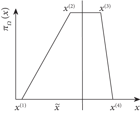
Remark 2. Notably, the above method is just the fuzzy logic [34] combining with Gaussian noise. The noises are modeled as several different Gaussian distribution intervals. In this article, however, we considered the situation, where noises obey possibility distribution instead of probability distributions. We modeled the noises as FRVs with the TPDs [29], which is an interval, but completely out of the Gaussian distribution. FRVs can be used to design FKF from the perspective of variable definition. For example, Sabzevari and Chatraei [29] set up FRVs and proposed the FKF for the Doris robot platform location.

Remark 3. FRVs can have many distribution shapes. We restrict the analysis to the trapezoidal distribution because in practical applications, no criterion exist to define the distribution shape between the possible and the impossible regions. The triangular, rectangular, and singleton distributions are particular cases of the trapezoidal distributions. For example, Shao et al. [21] use the maximum possibilistic informational distance principle to build a TPD from a set of data that follows unknown multimodal nonsymmetric probability distributions and to build a triangular possibility distribution from a set of data that follows a skewed normal probability distribution.

In particular, the objective of this paper is to formulate a stable fuzzy distributed filtering for a nonlinear system with fuzzy noise to ensure that each sensor i can increase its posterior estimate by fusing {z_j,k|k, R_j,k|k} and from neighbors based on the equation of system (8) and the equation of measure (9).

3. FCCIF

The proposed FCCIF contains two steps: prediction update and measure update. In the prediction update step, the predictive estimation set is obtained by fuzzy quadrature points calculating, fuzzy quadrature points propagating, and predictive estimation calculating. In the measure update step, the posterior estimation set is obtained by playing weighted average consensus on the prior information and novel information. The proposed FCCIF algorithm is of polynomial-order computational complexity [35].

1.
Prediction update: Let the prior state estimation of node i at time k − 1 is , and the initialized central gradient, uncertainty matrix, and fuzzy information matrix of are , , and , respectively.

Since the state variable is a fuzzy value following the TPD, the four vertexes of the volume point

can be calculated as

()

where e = 1, 2, ⋯, 2n, l = 1, 2, 3, 4. In Formula (12), S_{i,k − 1|k−1} represent the square root the uncertainty matrix; ξ_e is the e-th column of Matrix (13):

()

The fuzzy volume points propagating through the nonlinear equation can be calculated as

()

The volume point

will be used to calculate the TPD of the state prediction, while the central gradient

will be utilized to update the uncertainty matrix. Since the state prediction

obeys the TPD, it is sure that

()

is the center of gravity of the fuzzy state prediction. The fuzzy uncertainty matrix P_i,k|k−1, the fuzzy information matrix Y_i,k|k−1, and the fuzzy information estimation

can be calculated as

()

2.
Measurement update: The fuzzy volume points are recalculated as

()

where S_i,k|k−1 is the square root of P_i,k|k−1. The fuzzy volume points after propagation by the nonlinear equation can be calculated as

()

The fuzzy measurement prediction

can be calculated as

()

The cross-uncertainty matrix P_{xz(i, k|k − 1)} can be calculated as

()

Then, the fuzzy information vector

and fuzzy information matrix I_i,k|k−1 are estimated by

()

where

is the prediction error.

Therefore, the local estimated fuzzy information vector

and the estimated fuzzy information matrix Y_i,k|k can be obtained as

()

Afterward, the local information estimate can be updated using a weighted average consensus as (25):

()

A possible choice of the consensus weights can be [31]

()

Consequently, compute the posterior estimate

()

Then, the FCCIF algorithm can be obtained, as summarized in Algorithm 1.

Remark 4. To solve the strong nonlinear state estimation problems under the possibility theory, we put forward a new fuzzy cubature paradigm based on the volume filtering idea under the traditional probability theory. Different from the traditional volume filtering idea, the four vertices and the central gradient of the TPD need to select volume points and reconstruct through nonlinear propagation, so we call it a fuzzy cubature paradigm. Afterward, we propose a FCCIF by combining the average consensus algorithm and the FRV in distributed sensor networks on the possibilistic framework.

Algorithm 1: FCCIF algorithm for agent i at time k.

Input:The prior information
at time instant k − 1.
Prediction
Compute the fuzzy prediction estimation and
fuzzy information matrix Y_i,k|k−1 by equations (12)-(16).
Measurement update
(1) Compute the the local estimate set , Y_i,k|k by
equations (17)-(24).
(2) Perform consensus on the local estimate set by
equations (25)-(26).
(3) Update the posterior estimate by equations (27).
output: at time instant k.

4. Stability Analysis

Boundedness is an important feature of the algorithm stability. The FCCIF algorithm will be proven mean-square bounded through the Lyapunov analysis in this section [36]. The corresponding prediction estimate error and posterior error are expressed as and , respectively, where , , and x_k is the unknown real state. As mentioned in [20], the local observability assumption requires more communication among the sensors. Our algorithm only relies on the assumption of collective observability to guarantee its stability. The relaxation of the observability assumption reduces the quality requirements of the sensors. There are two preliminary assumptions as follows.

Assumption 1. The system is collectively observable, and the undirected graph is connected.

Assumption 2. The consensus matrix Π is primitive and row stochastic.

Now we give the stability result of the algorithm.

Theorem 1. The estimation error of FCCIF algorithm designed for nonlinear systems (8) and (9) is mean-square bounded.

To prove the above conclusion, an approximation of linearization is given first. The fuzzy pseudotransition matrix can be defined using the statistical linear error propagation methodology [37] as

()

where the uncertainty matrix

can be defined as

()

The fuzzy pseudomeasurement matrix H_i,k can be defined as

()

Therefore, Formulas (8) and (9) can be redescribed as

()

where the helpful matrix A_i,k−1 and B_i,k are brought in to counteract the possible errors in the approximation of linearization.

According to Equation (31), the fuzzy information vector and fuzzy information matrix can be redescribed as

()

Then, two important lemmas need to be given.

Lemma 1 ([38]). Let Assumptions 1 and 2 hold. Then, there exist positive definite matrices , , , and such that and for k ≥ 1 and any .

Lemma 2 ([39]). Given positive definite vectors v₁, ⋯, v_N and matrices M₁, ⋯, M_N for an integer N ≥ 2, the following inequality holds

()

Now, we can give out the proof.

Proof 1. We define for brevity. Here, stand for vertically concatenating all the vectors into a single column vector.

Let p be the Perron–Frobenius left eigenvector of the matrix

. Π^L is the Lth power of consensus matrix Π. According to Assumption 2, component p_i is strictly positive. And we have p^TΠ^L = p^T, that is,

. The estimation errors can be expressed as

()

where

()

Let us consider these three in (36) separately. Construct the collective dynamics of the first noise-free term as

()

where

Consider now the candidate Lyapunov function:

()

According to Lemma 1, we can see that there exist positive constants

making the following formula true

()

Based on Lemma 1 in [39], which imply for some

()

It follows that

()

where the last inequality comes out of Y_i,k|k≥

. Now, we apply Lemma 2 to get

()

Now, according to Lemma 1, we get that the noise-related term are bounded in mean square. Hence, Theorem 1 is proved.

5. Numerical Simulations

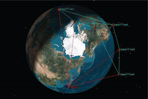
In this section, we will use space target tracking simulation to verify the effectiveness of the FCCIF algorithm. Consider the scenario as shown in Figure 2. There is a network of six space-based tracking satellites to track a noncooperative target through bearing-only measurement.

We first give the model of the noncooperative space target and the tracking satellites.

5.1. Dynamics of the Noncooperative Target

The dynamics of the noncooperative target can be given as

()

where r = [rx, ry, rz]^Τ is the position of the target,

is the velocity of the target, J₂ denotes perturbation, and μ stands for the gravitation constant. Let

denote the state parameters of the target in the geocentric inertial coordinate system. The state space model (44) can be expressed as

()

where harmonic coefficient a_J ≈ 0.00108263, E_r denotes the earth radius. The target dynamics only consider the Earth’s oblateness perturbation J₂, which is relevant for medium earth orbit (MEO). Thus, MEOs are a potential field of application for the filtering proposed in this paper.

Since the dynamic (45) is a continuous time model, (45) should be discretized. Set T = t_k+1 − t_k for the sampling period, the discrete model is described below:

()

where w is the process noise. When describing the motion of the satellite along the orbit, it is usually expressed in the form of six orbital parameters, namely, semimajor axis a_h, inclination u, eccentricity e, ascending node longitude Γ, perigee argument γ, and average anomaly m_h. Battistelli et al. [40] give out the nonlinear conversions that convert orbital elements to position and velocity.

5.2. Tracking Satellite Model

Satellites with optical sensors are used to measure the azimuth α or elevation β of the space target. The measurement Equation (9) can be concretized as

()

where

expresses the satellite’ position and va_k and vb_k express the measurement noise.

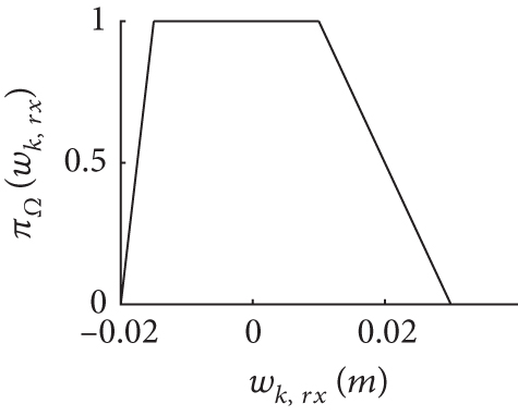
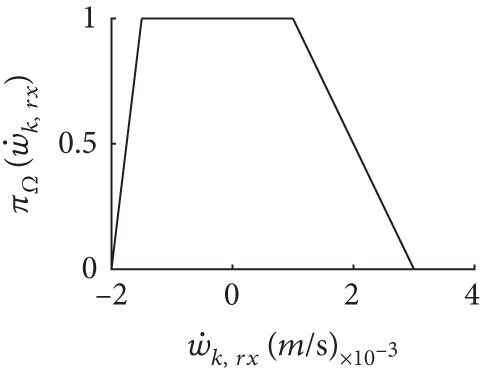
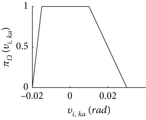
In general, and are modeled as Gaussian distribution. In this study, the noise terms w_k and v_i,k are modeled as FRVs with TPDs as Figure 3.

5.3. The Result of Simulation

The orbital elements of the tracking satellites and the space target are given in Table 1. The target’ initial state x₀ = [4619km, 3132km, 6630km,−5513m/s,−213.3m/s, 3942.6m/s]^T, sample time T_s = 3s, and total simulation time T_t = 900s. Since the initial states of the space target cannot be accurately obtained, they are set as x_i,0 = x₀ + Δx_i,0.

Table 1. Orbital elements of the tracing satellites and space target.

	a_h (km)	e	u (rad)	γ (rad)	Γ (rad)	m_h (rad)
Obj	8667.13	0	1.29	0.25	0	0.92
Sat1	9067.13	0	1.29	2.24	0	0.92
Sat2	8067.10	0	1.29	1.59	0	0.33
Sat3	8667.13	0	1.29	1.81	0	0.78
Sat4	8467.13	0	1.29	2.03	0	1.23
Sat5	8267.13	0	1.29	1.55	0	1.69
Sat6	9067.13	0	1.29	1.54	0	1.97

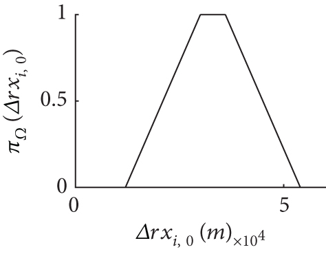
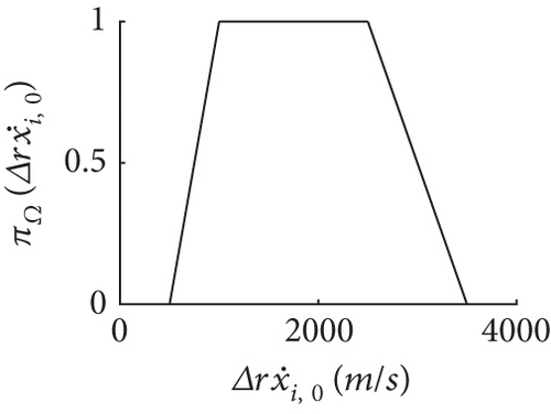
The initial errors are modeled as FRVs with TPDs shown in Figure 4. Then, and are the filter’ initial inputs.

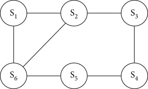
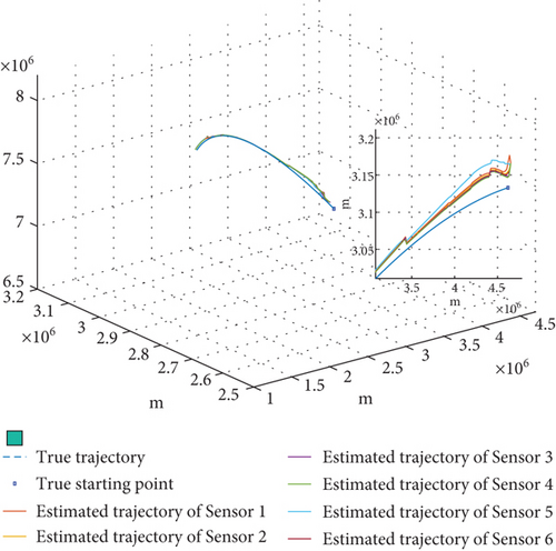
We use the fourth-order Runge–Kutta to make the prediction in FCCIF. The number of consensus iterations is L = 1, and the communication topology of the sensors is shown in Figure 5. By using these simulation settings, a random trajectory of the target was created. Subsequently, the trajectories estimated by each sensor are generated using the FCCIF algorithms as displayed in Figure 6. It is shown that the estimated trajectories generated using the FCCIF algorithms are close to the true trajectory.

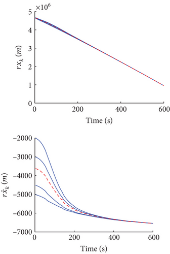
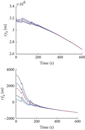
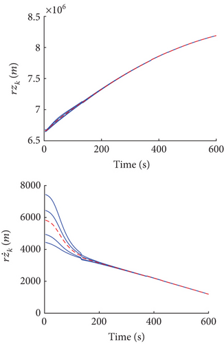
Figures 7, 8, and 9 illustrate the estimates of rx_i,k, , ry_i,k, , rz_i,k, and of the state value by Sensor 1. The solid lines respect the TPD of the fuzzy estimate value, while the dashed line respects the center of gravity of the fuzzy estimate value, that is, the final estimation of the state variable. The dashed line always lies within the solid lines stating that the final estimation is in an area of possibility. Moreover, as time elapses, the area of possibility shrinks, showing that the estimation is convergent. In addition, the area of the TPD is smaller than that of the noise TPD and initial error TPD. This indicates that the degree of fuzzy of the estimation decreases with filtering iterative. Moreover, the iterative distribution of TPD vertices becomes almost four parallel lines, and thus, the size of the possible regions is nearly invariant, which satisfies the requirement of coherence of the size of the regions [20]. Due to the length of the article, the figures for the estimates of the state value by other sensors are omitted.

Two hundred Monte Carlo simulations were conducted, and the mean square estimation errors (MSE) of sensor i were used to indicate the performance of the proposed FCCIF, which is defined as

()

The MSEP and the MSEV of sensor i can be given as

()

where

and

represent the true position vector and the true velocity vector, respectively. At the same time,

and

are the matching estimation of position and velocity of sensor i, respectively.

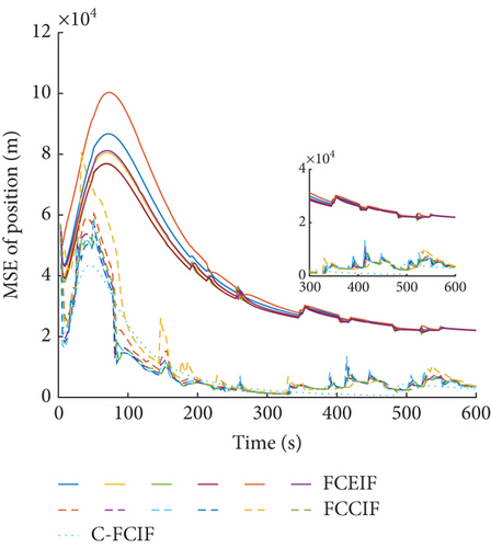
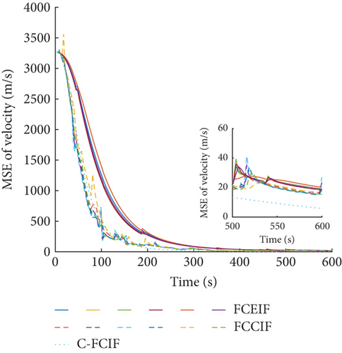
The MSE of position and velocity of six sensors are given in Figures 10 and 11. The results show that the proposed FCCIF has good filtering accuracy and stability. The results also show that the estimated values of six sensors reach a consensus, which achieves the purpose of distributed filtering. At the same time, for comparison, the MSE of the FCEIF, obtained by combing the DFIF in [32] and the EKF, and the centralized fuzzy cubature information filter (C-FCIF) are also shown in Figures 10 and 11. The prediction update of the FCEIF algorithm adopts the discrete model (47). Because of inadequate research on the C-FCIF, this study caused the FCCIF to degenerate to the C-FCIF by assuming that graph is strongly connected. Notably, the weight ω_ij,k in C-FCIF is set as ω_ij,k = 1/N instead of calculating as (26). The corresponding average MSE and percentage of MSE (PMSEP and PMSEV) are given in Table 2. It can be seen that the estimated accuracy of the FCCIF algorithm is close to that of the C-FCIF algorithm and increased more than the FCEIF algorithm, which has relatively large errors when ignoring higher order terms in Taylor expansion. The MSEP and MSEV of FCCIF are 23% and 90% of the FCEIF algorithm, respectively.

Table 2. Performance comparison in MSE.

Algorithm	MSEP (km)	MSEV (km/s)	PMSEP	PMSEV
FCEIF	22.4006	0.0183	100	100
FCCIF	5.1573	0.0165	23	90
C-FCIF	3.1955	0.0078	14	43

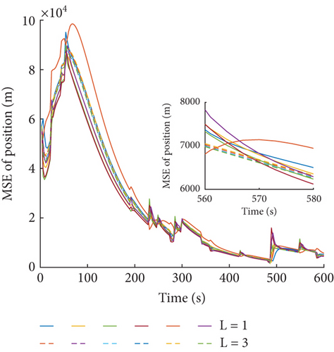
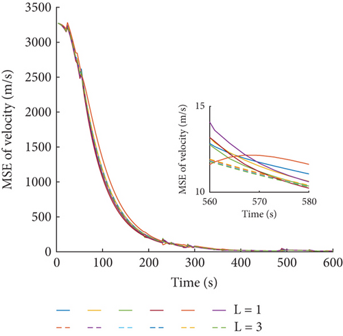
To analyze the influence of the consensus iterations on the estimated result of the FCCIF algorithm, the comparisons of MSE of the FCCIF algorithm with different consensus iterations L = 1 and L = 3 are as shown in Figures 12 and 13, respectively. The results show that as the number of iterations increases, the estimate accuracy improved, and the estimation errors of different sensors become more consistent. However, as the number of iterations increases, more time will be consumed. Therefore, it is necessary to select the appropriate number of iterations by considering the accuracy and consumption comprehensively.

Remark 5. We have not made simulation comparisons between the FCCIF algorithm presented in this paper and the CCIF algorithm in [13], the CCKF algorithm in [14], and so on, which were on the probability framework. It is because the possibility method does not always perform better than the probability method. Instead, we have to choose between these two types of approaches based on the types of knowledge available to describe the system. In applications where uncertainty is managed qualitatively, the possibility version makes more sense, while in applications where uncertainty is managed quantitatively [20], the probability version was more efficient.

Remark 6. As a limitation, the computation burden of FCCIF is significant than the traditional probability version, since all the updating of fuzzy variables must calculate the four feature points of the trapezoidal probability distribution. So the application of FCCIF, as currently formulated, is constrained in cases in which fast computation is required, for instance when dealing with truly big datasets. On the other hand, trapezoidal propagation is easy to cause deformation, which has very strict requirements on the set of initial value and noise parameters, so the convenience of practical operation needs to be further studied.

6. Conclusions

In this paper, the fuzzy noises are modeled as FRVs with TPDs instead of Gaussian distributions, so that the nonlinear estimated problem with fuzzy noises can be solved using a fuzzy cubature paradigm. A novel FCCIF algorithm is proposed by embedding the fuzzy cubature paradigm into the consensus frame. Moreover, under well-known observability and connectivity assumptions, the stability of the FCCIF algorithm is proven. Furthermore, it is verified that the estimated accuracy of the FCCIF algorithm is close to that of the C-FCIF algorithm and increased more than the FCEIF algorithm. The FCCIF algorithm needs to calculate the four feature points of the TPD for filtering iterative, and the calculation amount is larger than that of traditional Kalman filtering. Future work can be focused on examining if the efficiency of the algorithm can be enhanced using different fuzzy information fusion techniques. On the other hand, trapezoidal propagation is easy to cause deformation, which has very strict requirements on the set of initial value and noise parameters, so the convenience of practical operation needs to be further studied.

Conflicts of Interest

The authors declare no conflicts of interest.

Funding

This research received no external funding.

Open Research

Data Availability Statement

The data that support the findings of this study are available from the corresponding author upon reasonable request.

References

1 Oliva R., Blasch E., and Ogan R., Applying Aerospace Technologies to Current Issues Using Systems Engineering: 3rd AESS Chapter Summit, IEEE Aerospace and Electronic Systems Magazine. (2013) 28, no. 2, 34–41, https://doi.org/10.1109/MAES.2013.6477867, 2-s2.0-84897584957.
10.1109/MAES.2013.6477867
Web of Science® Google Scholar
2 Kennewell J. A. and Vo B.-N., An Overview of Space Situational Awareness, Proceedings of the 16th International Conference on Information Fusion, 2013, IEEE, 1029–1036.
Google Scholar
3 Weeden B. C., Cefola P. J., and Sankaran J., S. Ryan, Global Space Situational Awareness Sensors, Proceedings of the Advanced Maui Optical and Space Surveillance Technologies Conference, 2010, The Maui Economic Development Board, 14–17.
Google Scholar
4 Zhang P.-a., Wang W., Gao M., and Wang Y., Square-Root Cubature Kalman Filter Based on H Filter for Attitude Measurement of High-Spinning Aircraft, International Journal of Aerospace Engineering. (2021) 2021, 11, 5589691, https://doi.org/10.1155/2021/5589691.
10.1155/2021/5589691
Web of Science® Google Scholar
5 Liu B., Chen Z., Liu X., and Yang F., An Efficient Nonlinear Filter for Spacecraft Attitude Estimation, International Journal of Aerospace Engineering. (2014) 2014, 11, 540235, https://doi.org/10.1155/2014/540235, 2-s2.0-84897563091.
10.1155/2014/540235
Web of Science® Google Scholar
6 Teixeira B. O., Santillo M. A., Erwin R. S., and Bernstein D. S., Spacecraft Tracking Using Sampled-Data Kalman Filters, IEEE Control Systems. (2008) 28, no. 4, 78–94, https://doi.org/10.1109/MCS.2008.923231, 2-s2.0-48749133457.
10.1109/MCS.2008.923231
Web of Science® Google Scholar
7 Tian X., Chen G., Blasch E., Pham K., and Bar-Shalom Y., Comparison of Three Approximate Kinematic Models for Space Object Tracking, Proceedings of the 16th International Conference on Information Fusion, 2013, IEEE, 1005–1012.
Google Scholar
8 Wang S., Ren P., Takyi-Aninakwa P., Jin S., and Fernandez C., A Critical Review of Improved Deep Convolutional Neural Network for Multi-Timescale State Prediction of Lithium-Ion Batteries, Energies. (2022) 15, no. 14, https://doi.org/10.3390/en15145053.
10.3390/en15145053
PubMed Web of Science® Google Scholar
9 Zhou H., Huang H., Zhao H., Zhao X., and Yin X., Adaptive Unscented Kalman Filter for Target Tracking in the Presence of Nonlinear Systems Involving Model Mismatches, Remote Sensing. (2017) 9, no. 7, https://doi.org/10.3390/rs9070657, 2-s2.0-85022325776.
10.3390/rs9070657
Web of Science® Google Scholar
10 Arasaratnam I., Haykin S., and Hurd T. R., Cubature Kalman Filtering for Continuous-Discrete Systems: Theory and Simulations, IEEE Transactions on Signal Processing. (2010) 58, no. 10, 4977–4993, https://doi.org/10.1109/TSP.2010.2056923, 2-s2.0-77956781868.
10.1109/TSP.2010.2056923
Web of Science® Google Scholar
11 Chandra K. P. B., Gu D.-W., and Postlethwaite I., Square Root Cubature Information Filter, IEEE Sensors Journal. (2013) 13, no. 2, 750–758, https://doi.org/10.1109/JSEN.2012.2226441, 2-s2.0-84873172376.
10.1109/JSEN.2012.2226441
Web of Science® Google Scholar
12 Shao X., Li S., Zhang J., Zhang F., Zhang W., and Zhang Q., GPS-Free Collaborative Elliptical Circumnavigation Control for Multiple Non-Holonomic Vehicles, IEEE Transactions on Intelligent Vehicles. (2023) 8, no. 6, 3750–3761, https://doi.org/10.1109/TIV.2023.3240855.
10.1109/TIV.2023.3240855
Web of Science® Google Scholar
13 Jia B., Pham K. D., Blasch E., Shen D., Wang Z., and Chen G., Cooperative Space Object Tracking Using Space-Based Optical Sensors Via Consensus-Based Filters, IEEE Transactions on Aerospace and Electronic Systems. (2016) 52, no. 4, 1908–1936, https://doi.org/10.1109/TAES.2016.140506, 2-s2.0-84997706255.
10.1109/TAES.2016.140506
Web of Science® Google Scholar
14 Hu C., Lin H., Li Z., He B., and Liu G., Kullback-Leibler Divergence Based Distributed Cubature Kalman Filter and Its Application in Cooperative Space Object Tracking, Entropy. (2018) 20, no. 2, https://doi.org/10.3390/e20020116, 2-s2.0-85048379989, 33265207.
10.3390/e20020116
PubMed Web of Science® Google Scholar
15 Chen H., Wang J., Wang C., Shan J., and Xin M., Composite Weighted Average Consensus Filtering for Space Object Tracking, Acta Astronautica. (2020) 168, 69–79, https://doi.org/10.1016/j.actaastro.2019.06.033.
10.1016/j.actaastro.2019.06.033
Web of Science® Google Scholar
16 Hu Y., Su W., Chen L., and Liang Y., Cooperative Space Object Tracking via Universal Kalman Consensus Filter, Acta Astronautica. (2019) 160, 343–352, https://doi.org/10.1016/j.actaastro.2019.03.080, 2-s2.0-85065080991.
10.1016/j.actaastro.2019.03.080
Web of Science® Google Scholar
17 Jia B., Pham K., Blasch E., Chen G., and Shen D., Diffusion-Based Cooperative Space Object Tracking, Optical Engineering. (2019) 58, no. 4, 041607, https://doi.org/10.1117/1.OE.58.4.041607, 2-s2.0-85062612246.
10.1117/1.OE.58.4.041607
Web of Science® Google Scholar
18 Zhang Z., Li Q., Han L., Dong X., Liang Y., and Ren Z., Consensus Based Strong Tracking Adaptive Cubature Kalman Filtering for Nonlinear System Distributed Estimation, IEEE Access. (2019) 7, 98820–98831, https://doi.org/10.1109/ACCESS.2019.2929302.
10.1109/ACCESS.2019.2929302
Web of Science® Google Scholar
19 Zhou F., Wang Y., Zheng W., Li Z., and Wen X., Fast Distributed Multiple- Model Nonlinearity Estimation for Tracking the Non-Cooperative Highly Maneuvering Target, Remote Sensing. (2022) 14, no. 17, https://doi.org/10.3390/rs14174239.
10.3390/rs14174239
Web of Science® Google Scholar
20 Doostmohammadian M., Taghieh A., and Zarrabi H., Distributed Estimation Approach for Tracking a Mobile Target via Formation of UAVs, IEEE Transactions on Automation Science and Engineering. (2022) 19, no. 4, 3765–3776, https://doi.org/10.1109/TASE.2021.3135834.
10.1109/TASE.2021.3135834
Web of Science® Google Scholar
21 Shao X., Zhang J., Xu L., and Zhang W., Appointed-Time Guaranteed Adaptive Fault-Tolerant Attitude Tracking for Quadrotors With Aperiodic Data Updating, Aerospace Science and Technology. (2023) 132, 107881, https://doi.org/10.1016/j.ast.2022.107881.
10.1016/j.ast.2022.107881
Web of Science® Google Scholar
22 Serrurier M. and Prade H., An Informational Distance for Estimating the Faithfulness of a Possibility Distribution, Viewed as a Family of Probability Distributions, With Respect to Data, International Journal of Approximate Reasoning. (2013) 54, no. 7, 919–933, https://doi.org/10.1016/j.ijar.2013.01.011, 2-s2.0-84878584814.
10.1016/j.ijar.2013.01.011
Web of Science® Google Scholar
23 Matía F., al-Hadithi B. M., Jiménez A., and Segundo P. S., An Affine Fuzzy Model With Local and Global Interpretations, Applied Soft Computing. (2011) 11, no. 6, 4226–4235, https://doi.org/10.1016/j.asoc.2011.03.018, 2-s2.0-79956159534.
10.1016/j.asoc.2011.03.018
Web of Science® Google Scholar
24 Yang X., Wang S., Xu W., Qiao J., Yu C., Takyi-Aninakwa P., and Jin S., A Novel Fuzzy Adaptive Cubature Kalman Filtering Method for the State of Charge and State of Energy Co-Estimation of Lithium-Ion Batteries, Electrochimica Acta. (2022) 415, 140241, https://doi.org/10.1016/j.electacta.2022.140241.
10.1016/j.electacta.2022.140241
CAS Web of Science® Google Scholar
25 Xue M., Yan H., Zhang H., Li Z., Chen S., and Chen C., Event-Triggered Guaranteed Cost Controller Design for T-S Fuzzy Markovian Jump Systems With Partly Unknown Transition Probabilities, IEEE Transactions on Fuzzy Systems. (2021) 29, no. 5, 1052–1064, https://doi.org/10.1109/TFUZZ.2020.2968866.
10.1109/TFUZZ.2020.2968866
Web of Science® Google Scholar
26 Yan H., Xu X., Zhang H., and Yang F., Distributed Event-Triggered H_∞ State Estimation for T–S Fuzzy Systems Over Filtering Networks, Journal of the Franklin Institute. (2017) 354, no. 9, 3760–3779, https://doi.org/10.1016/j.jfranklin.2016.05.019, 2-s2.0-85008193273.
10.1016/j.jfranklin.2016.05.019
Google Scholar
27 Jwo D.-J. and Wang S.-H., Adaptive Fuzzy Strong Tracking Extended Kalman Filtering for GPS Navigation, IEEE Sensors Journal. (2007) 7, no. 5, 778–789, https://doi.org/10.1109/JSEN.2007.894148, 2-s2.0-34247170482.
10.1109/JSEN.2007.894148
Web of Science® Google Scholar
28 Yue Z., Lian B., and Gao Y., Robust Adaptive Filter Using Fuzzy Logic for Tightly Coupled Visual Inertial Odometry Navigation System, IET Radar, Sonar and Navigation. (2020) 14, no. 3, 364–371, https://doi.org/10.1049/iet-rsn.2019.0390.
10.1049/iet-rsn.2019.0390
Web of Science® Google Scholar
29 Sabzevari D. and Chatraei A., INS/GPS Sensor Fusion Based on Adaptive Fuzzy EKF With Sensitivity to Disturbances, IET Radar, Sonar and Navigation. (2021) 15, no. 11, 1535–1549, https://doi.org/10.1049/rsn2.12144.
10.1049/rsn2.12144
Web of Science® Google Scholar
30 Matía F., Jiménez A., al-Hadithi B. M., Rodríguez-Losada D., and Galán R., The Fuzzy Kalman Filter: State Estimation Using Possibilistic Techniques, Fuzzy Sets and Systems. (2006) 157, no. 16, 2145–2170, https://doi.org/10.1016/j.fss.2006.05.003, 2-s2.0-33746041454.
10.1016/j.fss.2006.05.003
Web of Science® Google Scholar
31 Ye D., Lin H., Yang X., He B., and Pan D., Spatial Target Localization Using Fuzzy Square-Root Cubature Kalman Filter, Proceedings of the 2016 31st Youth Academic Annual Conference of Chinese Association of Automation (YAC), 2016, IEEE, 73–80, https://doi.org/10.1109/YAC.2016.7804868, 2-s2.0-85011060242.
10.1109/YAC.2016.7804868
Google Scholar
32 Lin H., Hu C., Deng Z., and Liu G., Distributed Kalman Filter With Fuzzy Noises Over Multi-Agent Systems, IEEE Transactions on Fuzzy Systems. (2022) 30, no. 7, 2550–2562, https://doi.org/10.1109/TFUZZ.2021.3089038.
10.1109/TFUZZ.2021.3089038
Google Scholar
33 Zhang X., Lin H., Liu G., and Liu B., Distributed Kalman Filter With Fuzzy Noises Over Multiagent Systems Under Switching Topology, Digital Signal Processing. (2022) 122, 103326, https://doi.org/10.1016/j.dsp.2021.103326.
10.1016/j.dsp.2021.103326
Web of Science® Google Scholar
34 Zadeh L. A., Fuzzy Sets as a Basis for a Theory of Possibility, Fuzzy Sets and Systems. (1978) 1, no. 1, 3–28, https://doi.org/10.1016/0165-0114(78)90029-5, 2-s2.0-49349133217.
10.1016/0165-0114(78)90029-5
Google Scholar
35 Doostmohammadian M., Rabiee H. R., and Khan U. A., Cyber-Social Systems: Modeling, Inference, and Optimal Design, IEEE Systems Journal. (2020) 14, no. 1, 73–83, https://doi.org/10.1109/JSYST.2019.2900027.
10.1109/JSYST.2019.2900027
Web of Science® Google Scholar
36 Chen S. and Chen C., Probabilistic Fuzzy System for Uncertain Localization and Map Building of Mobile Robots, IEEE Transactions on Instrumentation and Measurement. (2012) 61, no. 6, 1546–1560, https://doi.org/10.1109/tim.2012.2186652, 2-s2.0-84862814206.
10.1109/tim.2012.2186652
Web of Science® Google Scholar
37 Zhang X., He B., liu G., Zifeng G., and Zhang X., Distributed Square Root Fuzzy Cubature Information Filter for Object Tracking on the Possibilistic Framework, IET Radar, Sonar & Navigation. (2023) 17, no. 4, 605–616, https://doi.org/10.1049/rsn2.12364.
10.1049/rsn2.12364
Web of Science® Google Scholar
38 Chen Q., Wang W., Yin C., Jin X., and Zhou J., Distributed Cubature Information Filtering Based on Weighted Average Consensus, Neurocomputing. (2017) 243, 115–124, https://doi.org/10.1016/j.neucom.2017.03.004, 2-s2.0-85015313666.
10.1016/j.neucom.2017.03.004
Web of Science® Google Scholar
39 Battistelli G., Chisci L., Mugnai G., Farina A., and Graziano A., Consensus Based Linear and Nonlinear Filtering, IEEE Transactions on Automatic Control. (2015) 60, no. 5, 1410–1415, https://doi.org/10.1109/TAC.2014.2357135, 2-s2.0-84928502344.
10.1109/TAC.2014.2357135
Web of Science® Google Scholar
40 Battistelli G. and Chisci L., Kullback-Leibler Average, Consensus on Probability Densities, and Distributed State Estimation With Guaranteed Stability, Automatica. (2014) 50, no. 3, 707–718, https://doi.org/10.1016/j.automatica.2013.11.042, 2-s2.0-84896759301.
10.1016/j.automatica.2013.11.042
Web of Science® Google Scholar

All articles

Fuzzy Consensus Cubature Information Filtering for Space Target Tracking

Abstract

1. Introduction

1.1. Notations

2. Preliminaries and Problem Formulation

2.1. Preliminaries

2.2. Problem Formulation

3. FCCIF

4. Stability Analysis

5. Numerical Simulations

5.1. Dynamics of the Noncooperative Target

5.2. Tracking Satellite Model

5.3. The Result of Simulation

6. Conclusions

Conflicts of Interest

Funding

Open Research

Data Availability Statement

References

Figures

References

Information

About Wiley Online Library

Help & Support

Opportunities

Connect with Wiley

Fuzzy Consensus Cubature Information Filtering for Space Target Tracking

Abstract

1. Introduction

1.1. Notations

2. Preliminaries and Problem Formulation

2.1. Preliminaries

2.2. Problem Formulation

3. FCCIF

4. Stability Analysis

5. Numerical Simulations

5.1. Dynamics of the Noncooperative Target

5.2. Tracking Satellite Model

5.3. The Result of Simulation

6. Conclusions

Conflicts of Interest

Funding

Open Research

Data Availability Statement

References

Figures

References

Related

Information