Optimization of Aerodynamic Design of a Winged UAV Through Genetic Algorithms and Large Eddy Simulation
Abstract
This paper focuses on the optimization of a winged UAV airframe utilizing a preliminary configuration and the combination of the Taguchi experimental design method and the evolutionary genetic optimization algorithm, along with computational fluid dynamics. Simulations were carried out based on the Reynolds-averaged Navier–Stokes (RANS) equations and SST k-ω turbulence model and the large eddy simulation (LES) for a speed of 50 m/s and a Reynolds number of 1.6 million. Optimization was conducted for six variables in a single stage, with 25 tests performed. The tested case is a winged UAV with a Lambda-shaped airframe design named SACCON, featuring wings with a tilt angle of 53°. The objective function in this study is the ratio of lift to drag specified. A genetic algorithm is used in conjunction with an initial configuration to create a new aircraft. Ultimately, the newly designed airframe demonstrates a 14% improvement in aerodynamic efficiency compared to the default state, and the lift-to-drag ratio increases by 55%, successfully concluding the optimization process.
1. Introduction
Aircraft designers in recent years have shown that the wing configuration is of great importance, with increasing focus from commercial, research, and military organizations. In this configuration, vertical and horizontal stabilizers are eliminated, leading to reduced wetted area and decreased flow interference over the airframe [1]. In this configuration, the airframe structure, that is, the fuselage and wing, is constructed as a single integrated unit, making the fuselage contribute significantly to lift generation. Enhancing lift production increases range, aerodynamic efficiency, and flight endurance [2–5]. The elimination of vertical angles in the fuselage reduces and consequently increases the radar cross-section (RCS) and stealth capabilities [6–8]. The mentioned features have led to the utilization of this configuration in commercial and military centers today for surveillance, tracking, and interception of winged UAVs in the form of unmanned aerial vehicles [9, 10]. An important aspect regarding this configuration is that, due to its extensive application in all aviation fields, aerodynamic efficiency, fuel consumption, and flight endurance are crucial; thus, optimizing this airframe has become significantly important for various purposes. Aerodynamic optimization has made significant advancements in recent years, and various methods have been developed, each with its own advantages and disadvantages. Research has been conducted in this field, some of which can be highlighted; in 1995, Quagliarella and Cioppa employed genetic algorithms (GAs) for the optimal design of a supersonic airfoil with the aim of creating a camber-less airfoil [11]. Optimization methods are used to find the best solution among a set of possible solutions. In engineering projects, decision-making involves identifying the optimal solution that meets certain constraints and objectives. Optimization methods can be applied to various types of problems, including linear and nonlinear programming, dynamic programming, and stochastic programming. The GA is a popular optimization method that simulates the process of natural selection and evolution. It was first introduced by John Holland in 1960 and has since been widely used in various fields, including engineering, finance, and computer science [12]. Uzun et al. proposed a new approach to modeling and controlling a morphing UAV. They created a dataset using Ansys Fluent and used artificial intelligence–based models to improve the performance of the UAV. The results show that the proposed model is more successful than traditional approaches and can estimate the swept angle required for minimum lift and minimize drag force [13]. Rodríguez-Abreo et al. developed a fuzzy controller system for a UAV, optimizing control gains using GA to minimize energy consumption [14]. Li et al. propose a novel approach to improve the efficiency of surrogate-based optimization in aerodynamic shape optimization, particularly in airfoils and wings. The method uses a deep convolutional generative adversarial network to generate realistic sample airfoils and a discriminative model based on convolutional neural networks to detect geometric abnormality quickly without expensive computational fluid dynamic (CFD) models. The proposed models are embedded in a surrogate-based aerodynamic optimization framework and demonstrate significant improvement in optimization efficiency compared to conventional methods [15].
Moghimi Esfand-Abadi, Djavareshkian, and Madani studied the effects of wing fences on wing tip vortices and control surfaces in a flying wing aircraft. They used a hybrid learning model to optimize fence placement and design, reducing the need for time-consuming CFD simulations. The approach led to significant improvements in preventing vortex engulfment and optimizing the split drag system [12]. Yin et al. utilized Fluent software and a GA-based program to optimize a three-dimensional wing, improving aerodynamic efficiency [16]. Jiangtao et al. optimized a critically supercritical wing using a combination of artificial neural networks and GAs to reduce shock wave strength [17]. Li et al. introduced machine learning techniques for aerodynamic shape optimization, improving efficiency twofold compared to conventional methods [15]. Guo et al. optimized a supersonic wing structure using a hybrid algorithm, increasing the lift-to-drag (L/D) ratio effectively [18].
The main objective of this research is to improve the aerodynamic performance and efficiency of high-altitude aircraft and, particularly, UAVs with this configuration through wing optimization using a two-phase algorithm based on GAs. To achieve this goal, considering the innovative methods developed and the large number of defined variables in this configuration, it was necessary to divide the variables into two categories and then optimize the UAV structure in two phases. Eleven variables were defined for this configuration, and due to the high number of variables, it was essential to split the optimization process into two stages. By using strategies and simulations based on CFDs, costs and time were significantly reduced. Therefore, the Taguchi design method was employed in this study, and the number of variables was reduced to six and five separately for optimization in two phases to present a fully matured design for the final configuration.
2. Sample Test
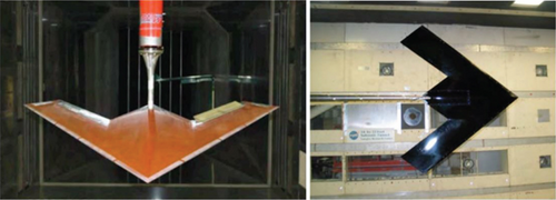
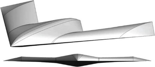
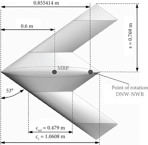
The geometry under investigation in this study is a UAV with a delta-shaped wing configuration called “SACCON.” This UAV utilizes wings with a 53° sweep angle. The UAV’s wing consists of three airfoils, with the first airfoil located at the wing root, the second airfoil in the middle of the wing, and the third airfoil at the wing tip. The third airfoil is angled at 5° relative to the horizontal to reduce drag. The study is conducted at a free stream velocity of 50 m/s. With an average chord length of 0.479 m for the wing, the Reynolds number is calculated at 1.6 million, and further details regarding the test conditions and the model are referenced in [19–22]. This configuration is composed of three airfoils in three sections, specifically tailored for this UAV. The protrusion present on the mid-body section is for mounting engines, communication systems, imaging equipment, and aligning the research features with operational standards. Figure 1 shows a view of the wind tunnel test model. Images of the wing configuration in Figures 1, 2, 3, and 4 and the geometric specifications of the wing in Table 1 are provided.
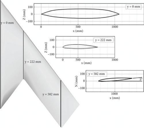
| Geometric component | Value (unit) | Symbol |
|---|---|---|
| Span length | 0.769 m | b |
| Wing area | 0.389 m2 | s |
| Sweep angle | 53° | Λ |
| Negative twist | −5 | θ |
| Reference chord | 0.479 m | Cref |
| Chord at symmetry line | 1.0608 m | Cr |
| Moment reference point | 0.6 m | MRP |
3. Numerical Solution
In this study, the flow equations are solved using the discrete finite volume method. To simulate turbulent flow, two models, large eddy simulation (LES) and SST k-ω, are utilized. The flow equations are solved in both time-independent and time-dependent manners. The SST k-ω turbulence model is used for time-independent equations, while the LES model is employed for time-dependent equations. The simple and coupled algorithms are utilized to couple velocity and pressure fields. The time-independent equations with the SST k-ω model are solved using the coupled method, while the time-dependent equations with the LES model are solved using the SIMPLE solver. A 5% turbulent intensity is considered in the simulations to ensure the best numerical results in alignment with experimental data. In this simulation, no-slip boundary conditions are applied to the body surface, and the Reynolds number is set at 1.6 million, corresponding to a flow velocity of 50 m/s. The working fluid used is air.
4. Design of Experiments and Optimization
- 1.
Input specification and limit definition.
- •
Inputs: The process begins by defining six input variables that represent the various geometric characteristics of the wing.
- •
Constraints: Constraints are established for each input variable to ensure that the resulting wing design remains physically within acceptable limits. These limitations may include factors such as manufacturing limitations, structural integrity, and aerodynamic stability.
- 2.
Output function.
- •
L/D as a function of output: The primary output of the optimization process is the L/D ratio. This metric quantifies the effectiveness of the wing in generating lift while minimizing drag. The output function defines how to calculate the L/D ratio based on the values of the input variables.
- 3.
Design of experiments.
- •
Taguchi method: The Taguchi method is used to design a set of experiments that efficiently explore the input variable space. This method helps to identify the most important factors affecting the L/D ratio.
- •
Experiments: A total of 25 experiments have been conducted, each with a unique combination of input variable values.
- 4.
Conducting experiments.
- •
Fluent software: The experiments were done using CFDs and Fluent software. A CFD simulation is used to model the airflow around the wing and calculate the resulting L/D ratio.
- •
Table of experiments: The results of each experiment are recorded in a table and provide data on the values of the input variables and the corresponding L/D ratios.
- 5.
Response surface fitting and sensitivity analysis.
- •
Response surface fitting: Data are analyzed to develop a mathematical model (response surface) that relates the input variables to the L/D ratio. This model provides the possibility of interpolating and predicting L/D values for any combination of inputs in the experimental range.
- •
Sensitivity analysis: This model is used to evaluate the sensitivity of the L/D ratio to changes in each input variable. This helps identify the most important factors that significantly affect wing performance.
- 6.
Optimization.
- •
GA: Evolutionary GA is used in this single-objective problem to optimize the L/D ratio. The algorithm iteratively generates and evaluates potential wing designs based on their L/D values and gradually converges on a near-optimal solution.
- •
Candidate solutions: The GA generates a set of candidate solutions, each representing a different wing geometry with its associated L/D ratio.
- 7.
Validation with Fluent.
- •
Aerodynamic analysis: Top-ranked candidate solutions are further aerodynamically analyzed using Fluent. This includes detailed simulations to evaluate their performance in various flight conditions.
- •
Comparison of results: The results of the validation process are compared with the initial design of the wing. If the optimized designs show a significant improvement in the L/D ratio, the optimization is considered successful.
- 8.
Selection of design points and production of new geometry.
- •
Design points: Based on the validation results, a set of design points is selected. These points represent the most promising wing geometry.
- •
New geometry: New wing geometries are created around these design points, potentially exploring a wider range of design possibilities.
- 9.
Aerodynamic analysis of new geometry.
- •
LES: New geometries are analyzed using advanced CFD techniques such as LES to capture more complex flow characteristics.
- •
Comparison of results: The aerodynamic performance of the new geometries has been compared with the initial design and the optimized candidates.
- 10.
Conclusion
- •
Optimization success: The optimization process is considered successful if the optimized geometries consistently outperform the initial design in terms of L/D ratio. The final optimized wing design can be adopted for further development or implementation.
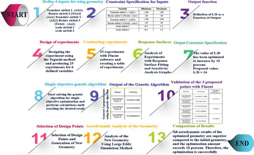
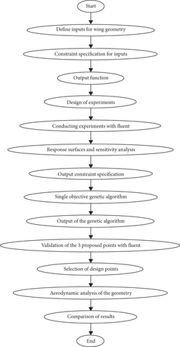
In summary, this workflow provides a structured approach to wing geometry optimization by systematically exploring the design space, evaluating performance metrics, and applying optimization techniques. A combination of experimental design, CFD analysis, and optimization algorithms enables the identification of improved wing designs that increase aerodynamic efficiency.
4.1. Learning Section
4.1.1. A Clear Overview of GAs and the Taguchi Method
4.1.1.1. GA [12]
- 1.
Begin with a group of organisms possessing arbitrary genetic makeup.
- 2.
Employ a fitness function to assess how well they performed.
- 3.
Choose the most fit animals to raise their progeny.
- 4.
Gene-swapping the chosen parents to create new offspring (crossover).
- 5.
Occasionally cause a mutation—small, haphazard alterations to the DNA.
- 6.
For several generations, repeat Steps 2 through 5.
- 7.
The population changes over time and improves its ability to handle the issue.
As the fittest organisms procreate and transmit their favorable genes to subsequent generations, the GA iterates this process and helps us find ever-better solutions throughout time.
4.1.1.2. Taguchi Method [23]
The Taguchi optimization formula is a mathematical formula developed by Genichi Taguchi, a Japanese engineer and statistician. The Taguchi optimization is used in the field of the design of experiments to help optimize product or process performance by identifying the best combination of factors for achieving the desired results.
The formula is based on the concept of signal-to-noise ratio, which measures the variability of a product or process output.
The S/N ratio is a measure of the quality of the output signal, with a higher ratio indicating better performance.
The n represents the number of experimental runs or trials conducted.
The yi represents the observed output value for each trial, which is compared to the target value T.
The target value T is the ideal or desired output that you are trying to achieve.
5. Solution Domain and Computational Mesh
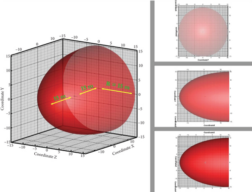
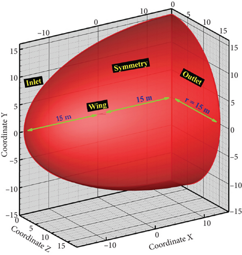
For the comprehensive simulation, a three-dimensional representation of the SACCON UAV is depicted in Figure 6. A domain with a rounded shape is utilized for the simulations, where the distance of the domain’s end from the aircraft body is set to 15 times the chord length of the UAV’s midline. The computational domain is illustrated in full detail in Figure 7. To reduce computational costs, the geometry is designed symmetrically around the axis, allowing the geometry to be modeled in a semihemispherical shape. The computational domain is semispherically designed around the UAV’s body for efficient calculations. The computational domain layout is presented in Figure 8, and detailed boundary conditions and domain specifications are provided in Table 2.
| Value | Fluent condition | Boundary condition | Boundary name |
|---|---|---|---|
| 50 m/s | Velocity inlet | Velocity inlet | Inlet |
| Gauge = 0 | Pressure outlet | Pressure outlet | Outlet |
| — | Symmetry | Symmetry | Symmetry |
| No slip | Wall | Wall | Wing |
6. Computational Mesh
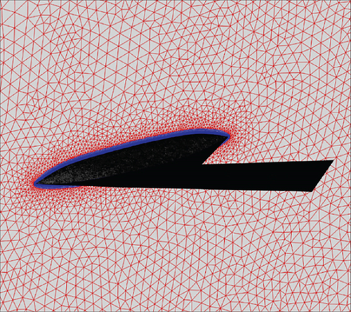
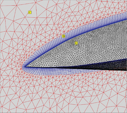
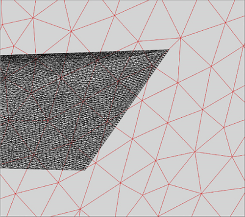
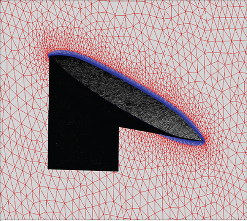
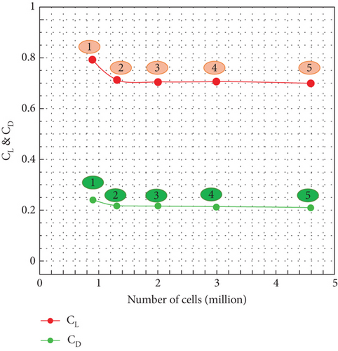
The computational mesh for the solution domain is a combination of structured and unstructured networks. Around the UAV, a boundary layer mesh consisting of 25 layers structured on top of each other has been established, and then an unstructured mesh is considered for the rest of the domain. In this work, Ansys Fluent software was used to generate a computational mesh for the analysis. This mesh discretization allowed for a detailed examination of key features within the domain. Figures 9, 10, 11, 12, and 13 present various views of the mesh. Notably, Figures 10, 11, 12, and 13 focus on a close-up of the wingtip region, highlighting the mesh refinement around the sharp corner. This refinement is crucial for capturing the complex development of the boundary layer in this critical area. Due to the geometric structure of the model and numerical solution requirements, the domain was meshed with tetrahedral, prismatic, and pyramid elements. Due to severe changes in velocity and pressure at the attack edge, escape edge, and wing tip, the mesh has been refined in these regions. It is worth mentioning that the mesh density has increased near the body surface to accurately model the physical phenomena in these regions. Based on Figures 9 and 11, the density in Regions A, B, C, D, and E varies, and a specific mesh density has been considered for each layer. For simulating flow and validation, a SST k-ω turbulence model was used, and for quality improvement of results, (y+) values for the entire boundary layer on the body were kept below 10. To ensure the accuracy and independence of results on the number of mesh cells, the values of the lift and drag coefficients were evaluated for five different mesh resolutions at a 20° angle of attack in Figure 14. This research was carried out using a grid with 3 million cells, which is suitable in terms of accuracy and computational load. In Figures 10, 12, and 13, a comprehensive visual presentation of multiple perspectives and intricate details regarding the solution method (meshing) employed in addressing the given problem is meticulously depicted.

7. Mesh Independence Study
To ensure the accuracy and independence of results from the mesh cell count, the values of lift and drag coefficients at a 20° angle of attack for 5 different meshes were investigated. Figure 14 shows the variations of lift and drag coefficients in relation to the number of mesh cells. For this study, Mesh Number 4 with a density of 3 million cells was used, which was found to be suitable in terms of accuracy and computational volume.
Furthermore, for simulating flow using the LES model, independence from the mesh was considered, and since this model is transient, independence from the time step is also necessary. The results for both mesh independence and time step independence for the LES model are shown in Figures 15 and 16, respectively.
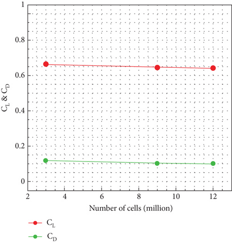

During these stages, the model with 3 million mesh cells is used for simulating both turbulence models. Additionally, a time step of 0.01 is used for the transient LES model.
8. Validation
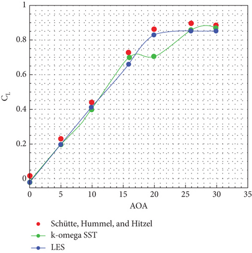
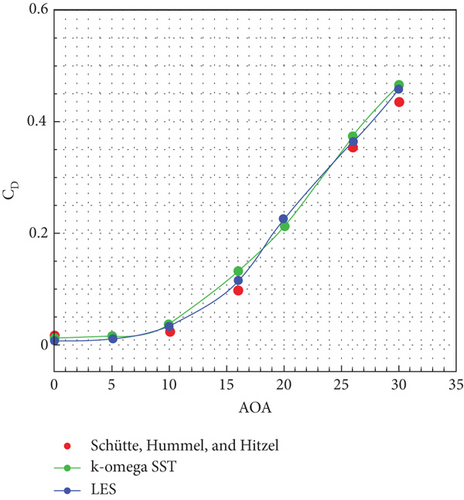
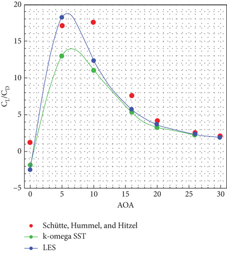
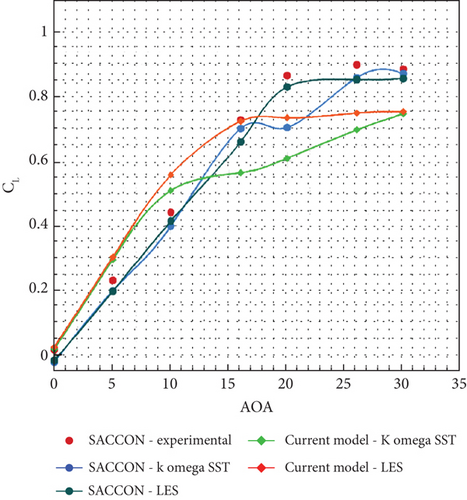
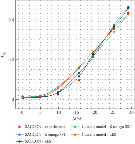
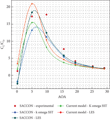
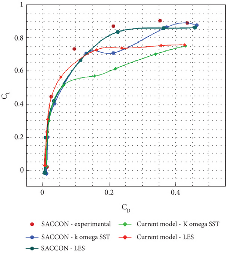
To conduct a detailed examination of the results obtained from numerical simulations, the values were compared with the experimental data available in reference [19]. As shown in Figures 17 and 18, the results for the lift and drag coefficients for both turbulence models are presented. It can be observed that the results are in very good agreement. The highest deviation was found for the SST k-ω turbulence model for a 20° angle of attack, with a magnitude of 18%. To address this issue, the LES turbulence model was also examined, which reduced the deviation to 4%. Figure 19 shows the comparison of lift and drag coefficient results for two turbulence models with experimental values. Figure 20 shows the comparison of L/D coefficient results for two turbulence models with experimental values.

9. Results and Discussion
9.1. Optimization and Airframe Design
The aim of this study is to design an optimal airframe using the optimization of another airframe. In this study, sections of the wing are specified, and variations in these sections are optimized using GA to optimize the UAV. In this research, three sections with six degrees of freedom are selected for optimization, reducing costs and computations using the Taguchi method and achieving a new airframe with much lower costs compared to previous methods. If a 20% increase in aerodynamic efficiency is achieved compared to the base state, the optimization goal has been satisfied.
9.1.1. Optimization Stage 1
In this section, the optimization of two wing sections with six degrees of freedom is carried out using the GA. Each section in this wing has three degrees of freedom, and their optimal values are evaluated using the GA. The process of this subject is then explained.
9.1.2. Degrees of Freedom in Wing
To optimize the aerodynamic structure of the UAV in cruise flight, angles of attack from 0° to 10° are considered. The cruise flights of aircraft are all defined within this range. The 5° angle of attack is selected from 0 to 10 as the base angle of attack and is considered a constant variable. From two perspectives, this angle of attack is significant: first, this angle of attack is in the middle of 0 to 10, and second, the maximum L/D ratio occurs at this angle based on the UAV’s features. Therefore, in all stages until the end of the article, all optimizations will be for a 5° angle of attack. The mission defined in all stages of optimization is the aerodynamic optimization of the UAV to increase range and reduce energy consumption. Here, the L/D ratio, or the ratio of lift coefficient to drag coefficient, is defined as the objective function in optimization. For geometrical optimization, six variables from the UAV’s geometry are chosen to conduct experiments with different values in the direction of optimization. These six variables include changes in displacement along the longitudinal axis, changes in the angle of attack of the airfoil, and changes in the scale size of the airfoil used for the intermediate and end airfoil sections, with three variables considered for each airfoil. The representation of these six degrees of freedom on the wing is shown in Figure 21.
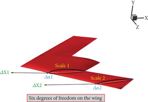
As shown in Figure 21, the six degrees are such that each of the two intermediate and end airfoils has three degrees of freedom, while the initial airfoil is fixed. The airfoils can move forward and backward along the longitudinal axis, and their angles of attack can rotate clockwise and counterclockwise with respect to the horizontal axis. Additionally, each airfoil can scale larger or smaller according to the constraints defined in the optimization design. As seen in Table 3, Airfoil 2 refers to the intermediate airfoil and Airfoil 3 refers to the end airfoil.
| Variable | Default | Minimum | Maximum | Unit |
|---|---|---|---|---|
| Translate Airfoil 2—(ΔX1) | 0 | −150 | 150 | mm |
| Rotate Airfoil 2 [twist]—(Δα1) | 0 | −10 | 10 | ° |
| Translate Airfoil 3—(ΔX2) | 0 | −150 | 150 | mm |
| Rotate Airfoil 3 [twist]—(Δα2) | 0 | −10 | 10 | ° |
| Scale Airfoil 2 | 1 | 0.5 | 1.5 | — |
| Scale Airfoil 3 | 1 | 0.5 | 1.5 | — |
9.1.3. Designing Experiments Using the Taguchi Method
The Taguchi method was utilized to design the tests, resulting in 25 stages of research. With this method, each of the six variables was divided into five parts, significantly reducing the number of tests to 25 stages instead of the initial 15,625 tests that would have been conducted without the Taguchi method. All tests were conducted using airflow with the SST k-ω turbulence model at a speed of 50 m/s and an angle of attack of 5°. After conducting the experiments, the L/D ratio was extracted and utilized for optimization.
9.1.4. Sensitivity Analysis of Variables and Response Surfaces
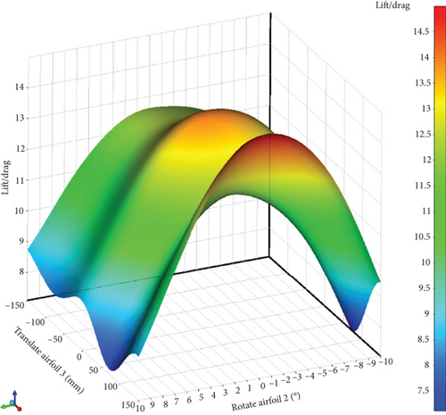
After doing the tests, the response surfaces for the results of each variable based on the L/D ratio are as follows: In Figure 22, four response surfaces based on the six defined variables are displayed, showing how each variable varies relative to another variable.
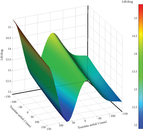
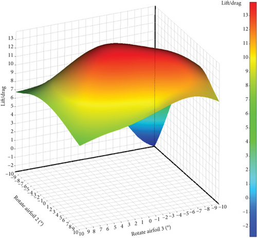
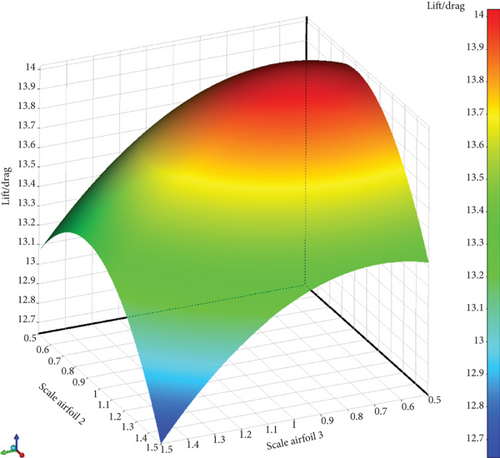
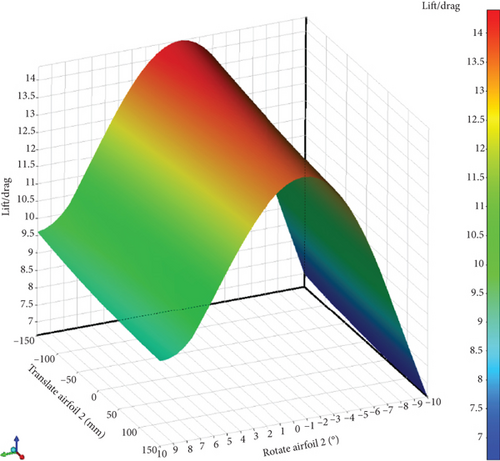
In Figure 23, the sensitivity level of the six variables is shown in percentage. It is evident from the above curve that the impact of each variable in the positive or negative direction will affect the output function. The first column from the right displays the sensitivity level of each variable on the lift force, while the second column shows the sensitivity of the variables on the lift force. In the first column, it can be observed that all variables have a positive effect on the lift force, except for the airfoil displacement in the longitudinal direction, which has a negative effect on the lift force and causes a reduction in lift. The same can be said for drag force: changes in all variables have a positive effect on drag force and increase it. However, longitudinal displacement reduces drag force. It should be noted that a decrease in drag force is desirable and an increase is undesirable. Therefore, this longitudinal displacement is desirable in the direction of reducing drag force, but changes in other variables that increase drag force are undesirable.
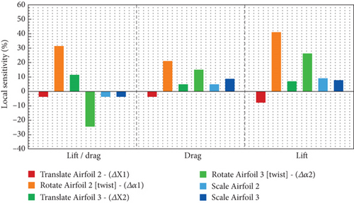
In the third column, the ratio of lift force to post force is shown. As observed, four variables have a negative impact on this ratio and decrease it, while two variables have a positive impact and increase it. The rotation of Airfoil 2 and the displacement of Airfoil 3 have a positive effect on the lift force–to–post force ratio and increase it. Next, the optimal design point will be found considering the above sensitivities using a GA.
9.1.5. Finding the Optimal Design Point Using a GA
In this step, the design point is found using a GA. Our output function here is to find the point of maximum L/D ratio. After performing the calculations, three design points are suggested by the GA, which are listed in Table 4. In the following, the validation of each one will be addressed, and ultimately proposed Design Point 1 will be chosen as the design point.
| Name | Translate Airfoil 2 (mm) | Rotate Airfoil 2 (degrees) | Translate Airfoil 3 (mm) | Rotate Airfoil 3 (degrees) | Scale Airfoil 2 | Scale Airfoil 3 | Drag (N) | Lift (N) | Lift/drag | Variation from reference |
|---|---|---|---|---|---|---|---|---|---|---|
| Candidate Point 1 | −149.4741279 | −1.038107105 | 149.1879232 | 0.533910828 | 0.804126997 | 0.66451627 | 11.60874627 | 145.2053007 | 15.62511496 | −2.21% |
| Candidate Point 1 (verified) | — | — | — | — | — | — | 9.6967393 | 148.16766 | 15.280153 | |
| Candidate Point 2 | −145.9897047 | −0.807624677 | 149.2716405 | −0.56360637 | 0.900883143 | 0.62826088 | 11.69795108 | 150.2902839 | 15.61222264 | −3.80% |
| Candidate Point 2 (verified) | — | — | — | — | — | — | 10.132593 | 152.18846 | 15.019696 | |
| Candidate Point 3 | −143.169141 | −1.124297809 | 149.8806623 | −0.129798835 | 0.88145426 | 0.631096885 | 11.59360116 | 148.3599922 | 15.60060327 | −3.48% |
| Candidate Point 3 (verified) | — | — | — | — | — | — | 10.170461 | 153.14339 | 15.057664 |
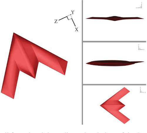
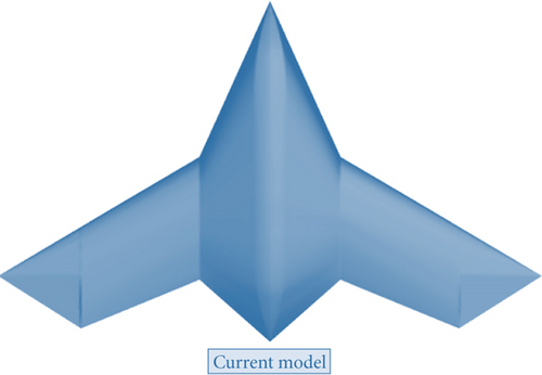
Based on Design Point 1, the newly constructed geometry is as follows: The new UAV is illustrated in Figure 24. This geometry is constructed with a smaller cross-sectional area, resulting in a reduction in volume and weight. This UAV’s frame is named Alpha.
9.2. Aerodynamic Analysis of the Alpha UAV Geometry
Next, simulation and analysis of the UAV geometry will be performed. Here, the new geometry will be analyzed using CFDs, and force diagrams of lift and drag, as well as their ratios, will be extracted.
As in Figure 25 shown in the images, a noticeable increase in the lift coefficient has been observed for both the 5° angle and the range of 0°–10°. The results of two turbulence models confirm these results. The drag remains constant at a 5° angle, and from 0° to 5°, this value remains constant, but it increases from 5° to 10°. The L/D ratio has increased for a 5° angle. The L/D ratio has increased from 0° to 7° compared to the SACCON model. Therefore, the current UAV named Alpha UAV has improved aerodynamic efficiency for its cruising range, which is a desirable effect, and the optimization has been successfully completed. Furthermore, the results of pressure coefficient contours along with streamlines for the Alpha UAV have been analyzed.
In Figure 26, pressure coefficient contours along with streamlines for the Alpha UAV are depicted. As evident, the pressure coefficient difference for the top and bottom surfaces of the wing has increased at angles from 0 to 10, leading to an increase in the L/D ratio. Additionally, the flow turbulence beneath the Alpha UAV’s wing has significantly decreased compared to the SACCON wing, resulting in reduced drag and ultimately an increase in the L/D ratio.
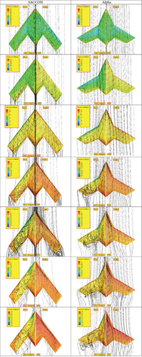
At a 0° angle of attack, near the wingtip region of the SACCON UAV, flow separation occurs, leading to reduced pressure beneath the wing. However, this issue has been resolved in the Alpha UAV, and there is no pressure drop. At 5° and 10° angles of attack, according to the contours, the pressure coefficient beneath the Alpha wing has increased, resulting in higher pressure compared to SACCON under the wing. Furthermore, a more significant pressure decrease is observed on the Alpha wing’s top surface compared to SACCON, indicating an increase in pressure and consequently an increase in lift for the Alpha UAV at all three angles.
Next, the extent of the lift coefficient increases and the ratio of lift coefficients to drag coefficients for the Alpha UAV compared to SACCON will be analyzed.
9.3. Level of Optimization for the Alpha UAV
In this section, a comparison between the SACCON and Alpha UAVs will be conducted, demonstrating the extent of improvement in both UAVs due to optimization. Tables 5 and 6 display the changes in the L/D ratio and lift coefficient variations at a 5° angle of attack for two turbulence models for the Alpha and SACCON UAVs, facilitating a comparison between the two.
| CL/CD | ||
|---|---|---|
| 5° AOA | SST k-ω | LES |
| SACCON Exp | 17.08826483 | 17.08826483 |
| SACCON | 13.03582113 | 18.23167649 |
| Alpha | 15.30819356 | 20.74121018 |
| Percentage change | 17.43% | 13.76% |
| CL | ||
|---|---|---|
| 5° AOA | SST k-ω | LES |
| SACCON Exp | 0.229709 | 0.229709 |
| SACCON | 0.19747736 | 0.19598436 |
| Alpha | 0.295068488 | 0.30335366 |
| Percentage change | 49.42% | 54.78% |
As indicated in Table 5, the L/D ratios for two turbulence models are displayed. According to this table, based on the SST k-ω model, Alpha’s optimization has resulted in over 17% improvement compared to SACCON and over 13% for the LES results. Referring to Table 6, the lift coefficient for the Alpha UAV based on the SST k-ω model has increased by over 49%, and according to the LES model, this increase is over 54%.
10. Conclusion
- •
In optimization, the scaling of wing section sizes had minimal impact on the L/D ratio, indicating that scaling on different wing sections is insignificant.
- •
The rotation of wing sections had the greatest influence on the L/D ratio, while the displacement of airfoils in the X direction resulted in minor effects. This applies to both the main wing and wingtips.
- •
The optimization in this study led to a 55% increase in the lift coefficient and a 14% increase in the L/D ratio.
- •
This optimization method, utilizing a combination of response surface methodology, Taguchi experimental design, GA optimization, and CFDs, proves to be highly successful and desirable. By incorporating LES modeling, the accuracy of the process and output results for design significantly increased, providing reliable outcomes.
Nomenclature
-
- AOA
-
- angle of attack
-
- CL
-
- lift coefficient
-
- CD
-
- drag coefficient
-
- Cref
-
- reference chord
-
- Cr
-
- chord at symmetry line
-
- MRP
-
- moment reference point
Conflicts of Interest
The authors declare no conflicts of interest.
Funding
No funding was received for this manuscript.
Open Research
Data Availability Statement
The data that support the findings of this study are available from the corresponding author upon reasonable request.


