1. Introduction

Since the electrical revolution, humanity has continually produced electricity by consuming fossil fuels, which has generated and releases significant amounts of carbon dioxide and had a profound impact on the environment. According to the International Energy Agency (IEA), the power sector is the largest contributor to global carbon emissions, accounting for 40% of total emissions in 2022, with this percentage trending upward [1]. Consequently, many countries and organizations have implemented measures to promote low-carbon reforms in the power industry. For example, Chinese government announced its “30–60” dual-carbon plan at the 75th General Debate of the United Nations General Assembly in September 2020 [2]. The UK government has introduced its 10 Plans for a Green Industrial Revolution in November 2020, utilizing over £12 billion of government funding to foster sustainable, future-proof green industries in the UK and worldwide [3].

With the increasing emphasis on the electricity carbon emissions, a rapid and high-resolution system for accounting and forecasting carbon emissions is crucial. In order to account the carbon emission in the electricity power industry, many researchers have conducted extensive studies. Currently, the carbon accounting methods can be divided into three main categories: emission factors method, mass balance method and monitoring method. The emission factors method is the most commonly used approach for accounting carbon emissions [4], which relies on constructing emission factors and activity data for each emission source [5]. The mass balance approach is another carbon emission accounting method which has been used in accounting carbon emission [6, 7]. This method allows for a quantitative analysis of energy consumption and carbon emissions throughout the entire energy input and output process [8]. The carbon factors method and mass balance method all rely on the statistical data of energy consumption and therefore they are not suitable for high-resolution (monthly and above) carbon emission accounting [9, 10]. To enhance the high-resolution carbon emission accounting, the monitoring method based on the continuous emission monitoring systems (CEMS) is proposed [11, 12]. However, the monitoring method is limited by the CEMS equipment costs and cannot be widely applied to large-scale carbon emission accounting.

In response, scholars have proposed a power carbon accounting method based on the carbon emission intensity of electricity to achieve high-resolution and low-cost accounting of electricity carbon emission [13]. The carbon emission intensity of electricity is defined as the amount of carbon dioxide emitted per unit of electricity consumed. It is used to obtain electricity carbon emissions by multiplying it with the electricity consumption [14, 15]. The feasibility of this method lies in the high real-time capability, accuracy, resolution, and wide collection scope of electricity data [16–18]. Currently, the carbon emission intensity of electricity is usually updated yearly [19]. However, with the rapid development of renewable energy, the carbon emission intensity of electricity may fluctuate significantly due to the uncertainty characteristic of renewable energy. The study result of [20] shows that there is a up to 30% error with using the conventional low-resolution carbon emission intensity of electricity for daily accounting of electricity carbon emission.

In order to achieve accurate high-resolution electricity carbon emission accounting, there is an increasing focus on the high-resolution forecasting of the carbon emission intensity of electricity [15]. According to the definition of carbon emission intensity of electricity, achieving high-resolution forecasting of carbon emission intensity requires a substantial amount of high-resolution electricity carbon emission data [21]. However, in many developing countries whose carbon accounting research started relatively late, it is challenging to be obtain enough historical high-resolution carbon emission data. Insufficient data prevents predictive models from fully learning, making accurate predictions difficult [22, 23]. Therefore, achieving high-resolution forecasting of carbon emission intensity of electricity in these countries faces significant data challenges.

In order to address these issues, an end-to-end monthly CIF method based is proposed in this paper, which consists of two main stages. In the first stage, we develop a high-resolution carbon emission data generator based on the correlation between electricity data and carbon emissions, thereby obtaining high-resolution historical carbon emission intensity of electricity data for training. In the second stage, a predictor is trained on the decomposed monthly dataset to achieve monthly CIF. In order to ensure that the decomposed data can improve the prediction accuracy CIF effectiveness, we integrate above two stages into a single end-to-end model, creating a feedback loop that simultaneously improves data decomposition and prediction during training.

The rest of this paper is organized as follows. Section 2 presents the implementation details of the proposed approach. Comprehensive simulation results based on actual data are reported in Section 3. Section 4 draws the conclusions and future works.

2. Methodologies

In this section, we first give the detail definition of carbon emission intensity of electricity and analyze the problems of the existing CIF methods. Then, the overall framework of the proposed CIF approach is introduced. Finally, all modules in proposed method are illustrated in detail, respectively.

2.2. Framework of the Proposed Approach

According to the above analysis, increasing the size of the historical monthly carbon emission intensity of electricity dataset is key to improving the forecasting accuracy of CIF model. As illuminated in Figure 1, the proposed CIF approach mainly includes two main steps: Data decomposition and Data-driven forecasting.

• •

  Stage I: Data decomposition. The first stage aims to generate more historical monthly electricity carbon emission data, then divide it by corresponding electricity consumption to obtain the monthly carbon emission intensity of electricity. In this stage, Denton method is adopted and improved as generator. This generator takes annual carbon emission data and monthly electricity consumption data as inputs and outputs monthly carbon emission data. The details of Stage I are described in Section 2.3.

• •

  Stage II: Data-driven forecasting. The second stage aims to achieve the monthly forecasting of carbon emission intensity of electricity. In this stage, the support vector machine (SVM) is used as forecasting model, and trained and optimized on decomposed monthly dataset. The details of Stage II are described in Section 2.4.

The separation of the two stages can lead to propagation errors, thereby affecting the accuracy of the prediction. To address this problem, we aim to integrate both tasks into one end-to-end learning model and optimized this model with the performance of predictor to achieve high accuracy of CIF. The details of end-to-end optimizing process are described in Section 2.5.

2.3. Denton Method-Based High-Resolution Data Generator

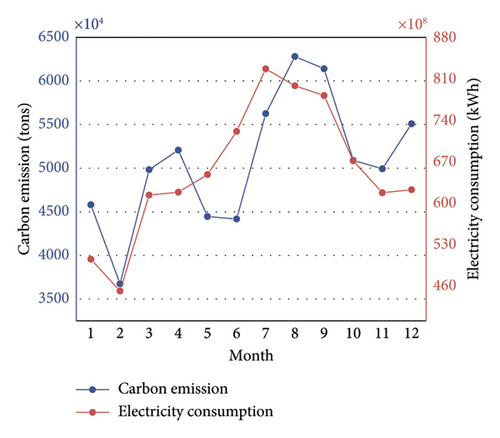
The Denton method is a nonsmooth data decomposition technique for time series data, commonly used to distribute low-resolution data into high-resolution data [24]. The key idea of the Denton method is to estimate data through high-resolution reference data relative with data to be decomposed. The decomposition process can be regarded as solving a constrained optimization problem which consists of three key parts: inputs, constraints, and objective function.

The inputs of generator are historical yearly carbon emission series and monthly electricity consumption. The output of generator is the monthly carbon emission. For any given year y, there is an annual total constraint between the annual carbon emission data and the monthly carbon emission data, as shown in equation (2):

$$ ()

The target of optimization is to make the generator decompose according to the temporal trend reference data. As shown in Figure 2, monthly electricity carbon emission data E^M has similar monthly temporal trend with monthly electricity consumption P^M. Based on above, the objective function of generator can be constructed as follows (3):

$$ ()

In summary, the entire optimization problem can be described as follows (4):

$$ ()

Therefore, the task of generator is to solve several simple constrained optimization problems. These problems can be solved quickly by using the least squares method.

2.5. Integrated Optimization

In our task, data decomposition and prediction are sequential steps, with the predictor’s performance being constrained by the authenticity of the decomposed data, but it cannot be ensured due to the lack of actual data. To address this issue, we propose an end-to-end model optimization approach, which feeds the performance evaluation of the downstream predictor back into the upstream data decomposition process and uses it as a target to guide the optimization of the decomposed data, thereby ensuring that the decomposed data can effectively enhance the accuracy of the predictions.

As illustrated in Figure 3, we input the high-frequency data, generated using the Denton method, from the generator into the differential evolution algorithm (DEA) model. The Denton method is employed to ensure that the high-frequency carbon emission data closely aligns with the actual monthly carbon emission factors, providing a meaningful initialization for the optimization process. This initialization not only improves the stability and convergence efficiency of the DEA but also reduces the risk of suboptimal solutions arising from poor initial values. The decomposed data is divided by the electricity consumption data to obtain decomposed carbon emission intensity of electricity data, which is then fed into the predictor for training. Subsequently, the predictor’s performance is evaluated on the actual carbon emission intensity of electricity dataset, and the evaluation result is fed back into the DEA to optimize the high-frequency carbon emission data. The loss of predictor can be calculated as (5) and the best loss on the validation set as the objective function of DEA is then fed back.

$$ ()

where L₁ is the number of samples in the valid set, $$ and $$ are the actual and forecasted monthly carbon emission intensity of electricity, respectively.

The DEA module is the key of integrated optimization method, we choose DEA as optimization algorithm since it has following two characteristics [28]:

• 1.

  DEA effectively explores the entire solution space through operations like mutation and crossover, helping to avoid getting trapped in local optima. This makes it particularly suitable for our global optimization tasks.

• 2.

  DEA has simple operational steps and requires only small amounts of computational resources, allowing to save significant time.

DEA is a population-based global optimization algorithm. As shown in Figure 4, DEA accept the decomposed data from generator into the DEA as the initial population and we use X⁰ to denote it. Generally, in the kth iteration, the current population is denoted as X^k. Then, the DEA mutates each element of X^k, using formula (6):

$$ ()

where f = 0.4 is the scaling factor used to adjust the magnitude of the mutation. $$, $$, and $$ are individuals randomly selected from current population X^k.

The mutation population V^k and the current popular X^k are combined through a crossover operation to generate the trial population U^k. The crossover operation is shown in formula (7):

$$ ()

where CR is the cross the crossover probability, in our paper CR = 0.3, rand (0, 1) means a random number between 0 and 1.

The magnitude of the trial population U^k+1 needs to be adjusted to meet the annual total constraint, specific operation is shown in formula (8):

$$ ()

The predictor is trained on $$ and its best loss on valid set is regarded as fitness of DEA. The DEA decides whether the trial population can become the new population X^k+1 based on the fitness, as shown in formula (9):

$$ ()

where fit_k is the fitness from the kth iteration, fit_k−1 is the fitness from the previous.

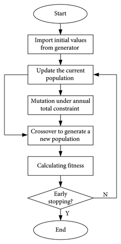
It is notable that DEA employs an early stopping mechanism to control whether the optimization process should be terminated. Specifically, the optimization stops if the DEA’s fitness does not decrease after 10 iterations.

3. Case Study

The case study is performed using Python 3.8 on a computer equipped with Intel Core i5-12400 CPU, 32 GB useable RAM and Nvidia RTX 3080. In this section, we first introduce the data set and accuracy assessments. Then, two cases are conducted based on the collected data.

4. Results

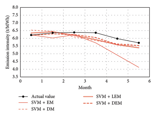
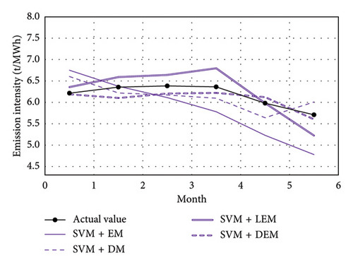
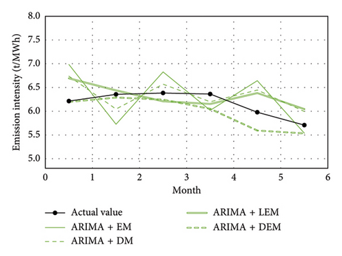
Figures 5(a), 5(b), and 5(c) show the forecast results using EM, LEM, DM, and proposed CIF method in three forecasting models, respectively. The evaluation metrics are enumerated in Table 1. It can be seen from Figure 5 that, compared with the EM method, all other methods provide more satisfactory forecast results, indicating that insufficient monthly data do not allow these models to be fully trained. Simulation results show that due to the increased scale of training samples from data decomposition, all three forecasting algorithms exhibit higher accuracy when using DM, LEM, and DEM compared to EM (see Table 1).

Based on the provided data, the predictive performance of different forecasting models and methods shows significant variation in terms of MAPE (%) and RMSE. Across all methods, the DEM consistently outperforms other approaches, achieving the lowest MAPE and RMSE values for all models, indicating its superior accuracy and reliability.

For the BP model, the DEM method achieves a remarkably low MAPE of 2.27% and an RMSE of 0.029, substantially better than the other methods, such as EM with a MAPE of 8.54% and RMSE of 0.110. Similarly, for the SVM model, DEM also performs best with a MAPE of 2.98% and RMSE of 0.020, compared to the EM method, which records the highest error metrics (MAPE 10.62%, RMSE 0.078).

The ARIMA model shows a consistent trend, where DEM achieves the lowest error values (MAPE 3.96%, RMSE 0.035), while EM yields higher errors (MAPE 8.13%, RMSE 0.071). Interestingly, the LEM and DM methods show competitive results across all models, with their errors generally lower than EM but higher than DEM.

These results highlight the superior performance of the DEM method in improving prediction accuracy across all tested models. This can be attributed to its ability to effectively capture dynamic and complex data patterns, making it the most reliable method among the options analyzed.

In comparing the models, SVM demonstrates overall superior predictive performance compared to BP and ARIMA models. Specifically, SVM achieves lower MAPE (2.98%) and RMSE (0.020) with the DEM method, while the best results for BP and ARIMA are 2.27%, 0.029 (BP) and 3.96%, 0.035 (ARIMA), respectively. Although BP slightly outperforms SVM in certain cases, its predictive performance is highly influenced by the choice of method.

The underperformance of BP compared to SVM is primarily attributed to overfitting. As a neural network-based model, BP is highly sensitive to the complex patterns in training data. When the sample size is insufficient or the data contains significant noise, the model tends to overfit the training data, leading to reduced generalization ability and suboptimal performance on test data. The experimental results indicate that although the Denton method was used to generate monthly carbon emission data for the past 10 years, the overall sample size is still insufficient to support the training of complex models such as neural networks.

Table 2 records the actual values and forecasting values of monthly carbon emission intensity of electricity using EM, LEM, DM, and DEM methods, while the best results under the same forecasting algorithm are in grey. It is obvious that the forecasting accuracy based on the proposed DEM method tends to be higher than others method in most months.

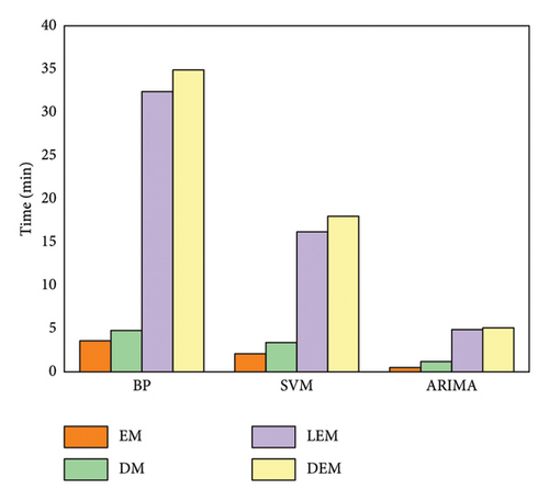
Figure 6 shows the comparison of the time consumption of different forecasting methods. It can be seen that all DEM and LEM method spend more time than all EM and DM method, which illustrates the integrated optimization consumed the majority of the processing time. In terms of forecasting algorithms, the BP model requires the most time (about 17 min). That is because the BP network has numerous hyperparameters and requires multiple training sessions with averaging to avoid unstable predictions. The ARIMA model requires the least time due to its simple structure and fewer hyperparameters (about 7 min). The SVM model, with its more complex hyperparameter settings, requires a certain amount of time (about 11 min) for optimization.

The experiments discussed above illustrate that the proposed DIE method can effectively improve the accuracy of monthly CIF.

5. Conclusion

In order to achieve accurate high-resolution CIF under limited high-resolution data, a data decomposition and end-to-end optimization-based monthly CIF method is proposed in our paper. Specifically, we design a high-resolution data generator based on ‘electric-carbon’ coupling characteristics and Denton method and integrate it with predictor into an end-to-end CIF framework. In this way, the performance evaluation of the forecasting task will guide the optimization of data decomposition. Therefore, the decomposed data are able to improve the accuracy of CIF effectively. We use actual monthly carbon emission intensity of electricity dataset to validate the proposed CIF method. The result shows that the proposed method can reach achieve satisfactory forecasting performance and provide a feasible approach for high-resolution forecasting of carbon emission intensity of electricity.

Conflicts of Interest

The authors declare no conflicts of interest.

Funding

This work was funded by the Science and Technology Project of BDC of State Grid Corporation of China, Project Name: Research on Key Technologies of Electricity-Carbon Market Collaboration Based on Green Electricity Contract, Grant No. SGSJ0000NYJS2400037.