1. Introduction

Off-grids are mostly dependent on stochastic RE power production. Their operational planning meets a high level of uncertainty in physical parameter dynamics related to chaotic variances in the environment. PQ estimations and the interpretation of results on daily bases are vital in scheduling of power consumption and selection of optimal consumer modes in smart detached networks contingent on RE. The proposed two-level procedure effectively examines various load-time schemes adapted to specific user demands in household use. Its daily PQ evaluation approves the selected scenarios in optimal system operation. Induction of intrinsic RE power can result in unacceptable PQ anomalies and states compared to traditional continual energy production. AI techniques can simulate or analyse statistical variances in PQ parameters on hourly or daily horizons according to historical records to eliminate their irregularities. Undefined weather anomalies in various modes of selected power consumers emphasise efficiency and PQ stability [1]. The reliability and effective lifetime of microsystems must be viewed from the points of view that balance RE power production and consumption. Detached microgrids that use RE are equipped with an integral battery backup to provide power supply in less favourable outside conditions. Power storage must face a higher degree of PQ optimisation in relation to variability in system charge states. Charge specifics and correlated power consumer collisions can produce additional PQ irregularities that cause system failures. The shift in the utilisation of equipment to times in a higher power supply optimises the PQ to avoid system instability. Dynamic management using combinatorial load scheduling algorithms focusses on efficient power use when considering RE and system capacity. It is based on switching on/off selected power consumers on user demand according to times in changed outside conditions. The load plans for active devices are continually reevaluated in a system that integrates environment monitoring. The selected load scenarios propose an optimal energy use according to battery backup and current RE production, to balance intermittent supply with user needs under various operating conditions [2]. Storage reserve units are recharged in excessive RE to support the system in supply shortages [3].

The research objective is a case evaluation of machine learning in predicting PQ day series bound on Numerical Weather Prediction (NWP) support and training time initialisation that adequately reflects local weather and binary load character. All possible time sequences of power demands are undefinable in an exact form, as the problem leads to a combinatorial explosion. Unpredictable RE production and operational conditions increase system irregularities, which are doubtful to be represented by conventional modelling. Optimal data interval series were initially identified to streamline regular training in full-model self-adaptation. The sampling initialises day-modelling periods according to detected error minima. The last observation series are test-used to eliminate model over fitting. The model is finally applied to 24 h forecast series, which replace the observational data of related variables used in the training. A regional NWP system can provide the final 24 h processing series. The trained PQ output is calculated at each prediction hour in full-day cycles. The sequenced computing procedure accelerates training and prediction, referring the observation input to the desired PQ output [4]. This hybrid strategy integrates the benefits of AI statistics, based on historical pattern learning capable of capturing local anomalies; and NWP physical large-scale simulation providing reliable mid-term forecasts. Their fusion eliminates unexpected cumulative ambiguities from statistical training, resulting from controversy or overbreak situations, but may magnify NWP local defects in causing less promptness in delivery in short time horizons in smart control. The models of compared advanced AI techniques produce similar output, except for a deep learning deficiency in voltage. The numerical results show DfL superiority and better stability in computing power (P) and power factor (PF) (avg. Root mean square errors [RMSE] = 0.29 kW and 0.032), while probabilistic learning predominates in approximate voltage-day cycles (RMSE = 1.95 V). Section 2 presents state-of-the-art, Section 3 standards in PQ, Section 4 data acquisition in an experimental smart grid, Section 5 methodology in day-ahead PQ validation, Section 6 computing AI methods, Section 7 data experiments, Section 8 experiments and results evaluation, and Sections 9 and 10 discussion and conclusion.

2. State of the Art in PQ Optimisation

An interactive self-triggering management in the PQ control identifies potential system violations and restores acceptable demand levels. Its sequential two-stage basis ensures initial generation resources and loads dispatched at minimal loss for system services; while in the second stage it evaluates PQ to determine whether the proposed solution complies distribution standards. A case study approved the use of parametric integrated tools in voltage balancing and harmonic distortion at optimal costs [5]. The intermittent nature of RE sources causes problems in the integration of electronic components with PVP systems, additionally affected by variability in user behaviour. Energy storage requires effective management to maintain grid PQ stability and balance power consumption under unexpected conditions, which can be obtained by active power filtering. Algorithms ensure stability and robustness in tracking the maximum power point of optimal energy distribution and system load management [6].

Automatic load classification combined with demand-response shedding can be used in smart grid optimisation based on the badger algorithm. Effective energy management optimises power consumption to minimise emissions, electricity costs, peak power demand, and power fluctuations in the integration of solar power with dynamic pricing. The topology was evaluated using MATLAB simulations, demonstrating superior performance compared to existing solutions [7]. Rapid dynamical changes in the environment induce discrepancies in PQ, mainly in harmonic distortion, sags, and swelling in RE based systems. MATLAB simulation under various conditions can help detect environmental factors implying power stability and system operability, such as the main contributing irradiance level that determines the maximum energy supply [8]. Optimal control schemes are implemented for RE power generation in grid side converters to ensure PQ issues. Various circumstances and effects on grid stability can be analysed in PQ record events to eliminate voltage fluctuation, harmonics, and flicker [9]. A novel energy consumption and PQ forecasting and monitoring tool is based on the polyexponential and random forest solution. An Internet of Things (IoT) framework integrated with RE forecasting improves load efficiency in buildings, by optimising daily energy consumption with PQ parameters [10]. A distribution microgrid could be controlled by active voltage filtering to stabilise the system operation. PQ management employs fuzzy logic to improve active energy conversion. The SIMULINK environment validated its effectiveness by improving the model using a neural network scrolling time frame that addresses nonlinearity and variability in the power supply [11]. Diverse sources of RE integrated into smart grids need to optimise load and demand management in sophisticated control strategies. The efficient use of distributed resources and storage units in the stabilised network is crucial to maximise power use and efficiency in system performance [12]. Multivariate long-short-term memory (LSTM) learning can improve resource management and energy use in smart homes in the realm of efficiency in system operation [13]. The efficient distribution of electricity in smart buildings is promising for reducing power dissipation and minimising energy loss. Predictions of dynamical stability in an IoT-driven approach, based on hyperparametric optimised gradient boost models, include the ability to return to a stable operating point after a disturbance event [14]. The deployment of deep learning models improves the accuracy of RE. Comprehensive operational planning in the AI-supported power grid ensures effective demand in robust electricity supply. Only a slight decrease in predictive precision can be observed along with an expansion of the time horizon [15]. Segmentation can diversify data into series of nonstationary character, while triggering can localise PQ spikes to recognise the time intervals of abnormal events and the primary errors. Periodical data can be transformed into Fourier series by assuming invariability in the frequency (Freq) domain. Transforms can improve the Freq resolution of time series to capture variational data [16]. PQ optimisation can employ spectral analysis with data sorting in series decomposition to identify the character of PQ patterns based on similarity. Finite-set element tools reduce steady-state signal harmonics [17]. Variations in photovoltaic (PV) supply can be assessed in categories using a probabilistic approach [18]. The pattern harmonics in PQ cycles could be recognised by Kalman filtering [19]. A stochastic load scheduling framework addresses the fast Freq response in capturing the inherent unpredictability of RE to characterise uncertainty in power consumption scenarios in low-inertia grids [20]. The inclusion of flexible load helps improve grid resilience and allows quick mode adaptation in response to Freq variations.

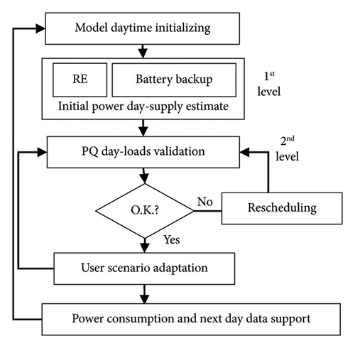
Mitigate PQ issues must be solved in optimal integration of generated RE and user demands aligned in load operating schedules of autonomous residential microgrids. The two-stage energy management algorithm guarantees the first energy resources and the secondary balancing loads at a minimum cost (Figure 1). The PQ is evaluated for several power consumption day scenarios at complied distribution levels. PQ optimisation generally integrates different AI approaches, whose hybrid algorithms are usually fully adapted to the case specifics. However, the solutions, in turn, lead to inconsistency in the undefined environment and configuration details. Aggregative probabilistic and LSTM learning are widely used and generally yields the best results. The novel DfL was designed to generally model dynamical uncertainties in any unknown system, and its modular concept based on partial differential equation (PDE) solutions was approved in the experiments. Optimal time shift at demand-side consumers ensures load-stabilised variant use in fault-tolerant RE grid supply. The key modelling time initialisation determines the applicability of detected training samples in a suitable predictive pattern representation. PQ and RE monitoring can be used to inform users, correct, and compensate for current deficiencies in energy production and backup support.

3. PQ Standardisation—Defining the Ranges

The power grid supply must comply with a continuous sine waved PQ voltage/current at the defined Freq to allow trouble-free operation at various user levels. The PQ parameters are standardised in ranges, allowing energy consumption/distribution without unexpected failures and loss in the life of system components. Unacceptable PQ spikes, abnormal from the defined forms, yield system dropouts or constraints in operation. PQ irregularities are fluctuations in PQ voltage/current from the desired sine wave, possibly resulting in system instabilities or misfires in the user-load modes. Undesired variances in PQ magnitudes are primarily a result of rapid dropout changes in the power supply/switching load that normally occur in RE production/consumption [23]. The nominal operational deviations for the voltage/current and the derived PQ characteristics are defined in the norms. European EN 50160, IEEE 1159. They standardise the PQ in relation to the limitation thresholds (voltage, current) in relation to the operational states in nominal time changes (Table 1). The PQ norms comprise a wider range of problems, including various scales of range in time sequences to reach a steady state [22]. The PQ parameters characterise the stability of units in intermittent RE supply along with various charge states in equipment load schedules [24].

4. PQ and Environmental Data Measurements in an Experimental Smart Off-Grid

The PQ data were obtained from the SMC measuring component on microscale sampling. Different combinations of 4 types of household appliances were switched on/off in various sequences of PQ monitoring (Table 2). The load of 4 combined pieces of equipment related to the PQ is the result of a different state of charge (SoC) directly related to the operational and environmental framework. The battery units were recharged in different periods and times with respect to the RE peak supply to optimise the SoC for the planned and predicted power production in unsettled weather. SoC data (storage level) were not recorded in this case study (Figure 2).

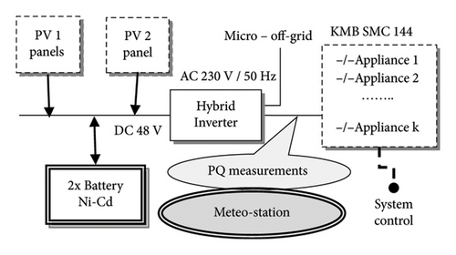
Minute-sammpled series of average voltage (U), total harmonic distortion—voltage (THDU), PF, P, total harmonic distortion-current (THDI) and freq were recorded in four different load combination sequences of switching usage. The harmonics of the THDU and THDI series were observed and evaluated in the system for each active household appliance separately as the main voltage/current component [25]. The increase in voltage is induced by the variability in the load of the equipment [26]. The observed Freq fluctuations are in the nominal ranges of 49.95–50.04 Hz of the acceptance limits (Table 1). Observational 5 min series of standard meteorological quantities: avg. ground temperat., relat. humid., atm. Press, wind and gust, precipitation and radiation parameters were recorded in the system with PQ measurements, as PVP is related to the environment potential. Modelling PQ using training statistics on historical records requires a detailed series to capture fluctuations and anomalies in patterns, which improves the approximation of ramping events.

The autonomous house simulation system is equipped with two PV panels based on fixed monocrystalline stable construction and one polycrystalline type placed on a tracker for higher efficiency in its conversion. Each of them is capable of a peak supply of 2 kWp (kW peak hour) of power. Both PV panels are connected to the system through a frequency converter in the DC transmission BUS. The AC hybrid inverter connects all appliances (in real and apparent power) controlled by a switchboard software system. The connection of the off-grid to a conventional distribution network is necessary due to inadequate supply of RE under real operational conditions, but the experimental study is based only on detached RE supply. A weather observation station is built in part of the off-grid power system [27]. Each individual power consumer is connected to the system through the AC BUS and is controlled according to its connection priority, load character, potential RE supply and SoC. Energy storage comprises two Ni-Cd accumulators consisting of four parts, each of them including four battery units. The delay effect of this type of backup essentially influences maximum storage capacity in repeating recharge cycles, leading to a dropout of the available storage capacity if discharged in a partial measure [28].

5. Methodology in Daily PQ Estimation of PQ for Various Untrained Load User Consumers and NWP Data

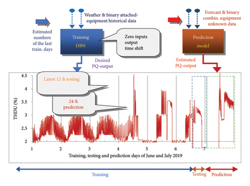
Differential modular, LSTM deep and stochastic learning based on statistical regression were used to model real weather and PQ measurement input-output data relations. The time delay between the model input and the target PQ output is set to zero; NWP data replace standard meteorological observations in the final prediction stage. A complement testing procedure based on the last-data model validation allows us to avoid overfitting. This approach optimises processing unknown 24 h NWP replacement series, produced by a regional forecast system. The trained PQ target is predicted at the same time points in one processing sequence stage.

The applicable day training periods are preassessed by initialisation times, in examining the complete data series in a sequenced detection for intervals of increasing 2 to k days. Continuously evaluated testing minima in the latest available day-afternoon hourly data denote the optimal day series of training samples. These day-range estimations allow for adequate patterns representation of input-output correlations in processing of unknown prediction data. After training, the AI statistics model is applicable to the corresponding NWP series (Figure 3), which reduce chaotic dynamical changes and uncertainty in breakover and unexpected ramp fluctuations in estimating the target PQ in a 24 h day horizon. The model input consists of relevant standard weather observations which are sampled at the 5 min time stamps (7 + 1 data quantities) and 4 binary combinatorial series indicating the switching equipment (Section 4). PQ input data are not used in learning due to missing measurements, that is, the unavailability in prediction times. The decimal indicates the four combined switches on consumers from the 10 connected appliances, to extend the standard binary input that can improve the prediction of PQ (Table 2). The sampling time relates harmonics of the target wave PQ parameters to input, which is important to properly characterise day PQ-periods. Power consumers combined at an utilisation time represent specific loads according to the collision character. An operational state is determined by binary combinatorial indicators of the attached equipment in various weather and SoC. All binary load patterns in deterministic definitions are not available when formulating a problem for dozens of possibly connected consumers to the grid. The number of possible combinatorial inputs increases exponentially in a specific user mode. PQ predictions on day horizons simulate various unforeseen states of the system and indicate an eventual collision related to component characteristics in the active regime.

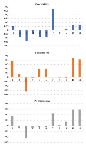
The weather input and the PQ output data are analysed in Figure 4; the degree of correlation indicates a positive (+1) or negative (−1) one between two quantities. The positive (negative) correlation indicates that if the values in the first array are > 1, the values in the second one are > 1 (< 1 or contrary). A coefficient value close to 0, denotes no or tiny correlation. The solar zenith angle determines the intensity of radiance under different light conditions in the atmosphere. The clear sky index (CSI) accounts for this phenomenon by expressing the relative PVP data in a ratio of training and prediction processing time. The actual solar radiation or PVP series is related to the time maxima when considering the ideal clear sky at each hour. Absolute global radiation was standardised to CSI series used in modelling on the data scale < 0, 1 >. Cyclic data from CSI norms are incorporated into their relative values to compensate for changes in the diurnal periods of the day cycle. CSI maximal series were determined to normalise data series, first searched and detected algorithmically in available seasonal data sets considering sampled times [29]. RMSE are the standard criteria for model validity in machine learning and testing approval of the models to unseen prediction data.

6. Differential Modular, Long-Term Deep Regression Tree Learning Statistics

6.1. Differential Binomial-Network

Differential Binomial Tree Network (DBN) is an unconventional hybrid neuro-computing regression technique, designed by the author, which combines machine learning based on AI with numerical mathematical procedures. DBN parses the general linear type of the kth order PDE (1) into simplified 2-variable PDE converts transformed nodes of a recognised order. DBN can model uncertain and chaotic dynamic systems whose behaviour is difficult to express by an exact mathematical definition. The evolution of the DBN model comprises efficient feature extraction that overcomes conventional regression and AI computing that require additional preprocessing of data input. It gradually develops multilayer binomial tree (BT) frames, by adding nodes one by one into the processed layers, to form and select applicable PDE modules in the BT nodes. Modules are tested and selected to be added or extracted from/from the model sum to calculate and reach both training and testing error minima. Progressive model expansion using the PDE concept usually allows one to find the optimal solution to machine learning problems using Goedel’s incompleteness theorem. Each node in BT selects the best-fit input combinations, produced by previous layers, to determine a form of sub-PDEs according to Operational Calculus (OC) procedures. DBN models can represent highly nonlinear and complex systems, described by dozens of data variables and hidden correlations. The order of binomials is related to the transformed PDE order [30].

$$ ()

A, B, …, G are functional coeff. of the inputs x₁, x₂.

The OC procedure applied to the derivatives of f(t) in a PDE (1) assumes that the resulting nth Laplace transformed derivatives can be converted into polynomial form (2), taking into account the defined beginning states (4).

$$ ()

f(t), …, f⁽ⁿ⁾(t) are originals continal in < 0+, ∞ > p, t—complex and real inputs.

The derivatives of f(t) can be converted to the OC to form mathematical equation (2), where the L-form of F(p) is formulated by a complex definition p as a simple ratio (3).

$$ ()

B, C, A_k—elementary fraction coeff. a, b-. param. of polynomials α₁, α₂, …, α_k—roots (real).

The ratio equations correspond to the originals of the L transform function f(t), which requires the inverse operation employing OC definitions (2) and (4) to restore f(t) in the nontransform by solving the initial PDE (1) in this way.

$$ ()

P(p), Q(p)—multinomials of degree s − 1, s. α₁, α₂, …, α_n—simple real roots of Q(p).

In the case f(t) can be expressed in a periodic form, the derivatives are transformed into sine- and cosine-convertible PDEs (5) and the original restored analogously (4). This extension expression is applied to the frequencies and amplitudes of periodic data to represent the L-images of unknown node function origins.

$$ ()

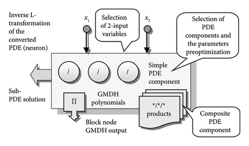
The inverse operation L on the ratio (4) or periodic term, resulting from PDE substitution, yields the searched functions (5). The restored originals of two-variable functions u_k are produced at selected BT nodes (Figure 5) and summed in the separable output model u defined by the PDE (1).

Pure rational y_k terms (6), composed of multinomials of the n − 1 and nth degree in the numerator and denominator, result from converted 2-variable node sub-PDEs. Appropriate first- or second-order polynomial members are tested in the numerator to form substitution ratio terms. The complete polynomial in denominator is used to calculate the node output (with the shared parameters in blocks).

$$ ()

y_j—particular sub-PDE solutions of unknown node u_k functions sig—sigmoidal transformation. φ = arctg(x₂/x₁)—phase of two-input variables x₁, x₂. a_i, b_i, w_j—polynomial parameters and term weights.

If the input has a circulate character, its node PDE can be substituted by sine/cosine transforms to calculate the original by the reverse e function (5). This expanded definition can be applied in processing the amplitudes and phases of periodic data (e.g., wind azimuth, radiation, etc.) to obtain adequate L-substitutes in periodic form for x₁, x₂ PDE nodes.

$$ ()

y_i—periodical L-transform node PDE-term, γ–phase variable [radian] x₁, x₂—amplitude, a, b—parameters.

The representation of the Euler form complex number c (8) in polar coordinates is related to the definition of f(t) (4). The parameter r (i.e., radius, part of the amplitude) is related to the term of the ratio and the angle (a part of the phase) = arctg(x₂/x₁) of two inputs from the real nodes x₁, x₂ determines the original f expressed in converted F(p) (5).

$$ ()

x₁ = Re, x₂ = Im.

The proposed innovations in the DBN design, which:

• ✓

  forms adding node-by-node a BT structure to parse the n-variable PDE of a general order into a node group of adaptable determined sub-PDEs.

• ✓

  produces optimal sub-PDE modules using rational, power, and periodic substitution in BT nodes.

• ✓

  OC conversion of periodical PDE forms, using the L-transforms, is used in modelling of periodical data variables (e.g., PVP, solar radiation) combined with angle data (e.g., wind azimuth) and time.

• ✓

  spreads progressively the modular PDE model using Goedel’s incompleteness optimisation, increasing step by step the complexity of a model structure.

• ✓

  employs an iterative optimisation procedure inserting PDE node solutions by eliminating redundant ones (from previous layers), in synchronising active nodes (reducing the components in BT structure).

6.2. Long-Term Deep Learning MATLAB

The Deep Learning Toolbox (DLT) in MATLAB enables sequence-to-sequence regression based on a default LSTM architecture¹. DLT net layers consist of:

• ➢

  A Sequence input-layer

• ➢

  A LSTM-layer

• ➢

  A Fully connected layer

• ➢

  A Dropout-layer

• ➢

  A Fully connected-layer (regress. output)

• ➢

  An output regression layer

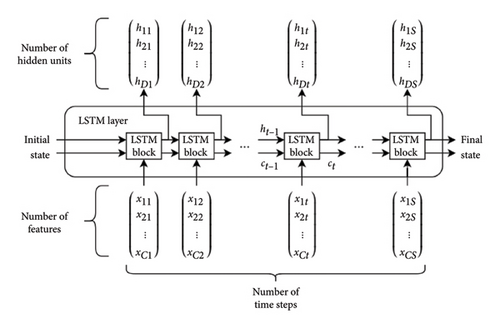
The input sequence and the LSTM layers are the two key processing components of the DLT. The sequenced input layer provides time sequences of data to the main layer of an LSTM network, which is trained to long-term correlations of sequenced data at successive times (Figure 6).

6.3. Probabilistic and Ensemble Machine Learning of MATLAB

The MATLAB regression statistics machine learning toolbox (SMLT) evaluates the performance of its statistical models in predicting/estimating the target output parameters. SMLT comprises a variety of conventional, hybrid, ensemble, and stochastic techniques²:

• ❖

  Regression-linear (interact., robust, stepwise)—using a simple constrained expression with linear parameters.

• ❖

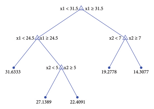
  Regression trees (fine, medium, coarse)—the branches are built and followed in a root-leaf node 2 decision way considering the estimated output of a predictor (Figure 7).

• ❖

  Support Vector Machine (SVM)—linear, Gaussian, or Radial Basis Function (RBF), quadratic, cubic kernels define the nonlinear transform functions applied on data in the stage of pretraining.

• ❖

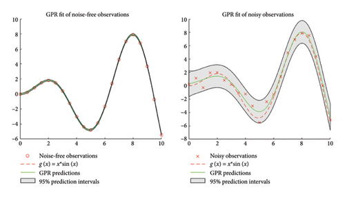
  Gaussian Process Regression (GPR)—a probability over the definition space is determined by a distribution function (Figure 8) used to compute the model output. A base function (zero, constant, linear) defines specific of the mean prior model forms⁴.

• ❖

  Ensemble-Bagged or Boosted Trees (EBaggT or EBoosT) fuses the output from single self-standing tree ensembles. Least-square expansion, bootstrap bagging, and aggregation improve the predictive performance of the model in a probabilistic output³.

SMLT built in Principal Component Analysis (PCA) can extract data input; however, it did not improve the model performance². The final SMLT models were chosen to achieve a testing error minimisation to process unseen data in the final PQ prediction.

7. PQ Day Prediction Processing NWP Data for Unknown-Powered Consumers—Experimental Studies

The AI models predicted parameters U, THDU, P, PF and THDI of PQ daily using the proposed modelling procedure (Sect.4) in the detached grid microtesting facilities (Figure 2), of VSB-TU Ostrava, Czech Rep., Ostrava-Poruba, during the 10-day experiment period 29 June–8 July 2019.

The 1 min PQ data recording was interrupted by some dropout failures in power status in several measuring time intervals, leading to a loss in data minute sequences on June 19 and 20. Corrupt records (set to zero values) are interpolated; however, these replacement data are not applicable in training⁵. The data set consists of archive series 14 June–12 July 2019, 8352 5 min sampled avg. all.

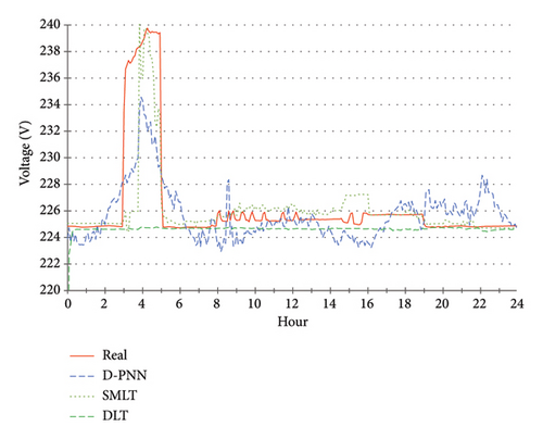
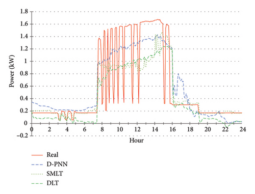
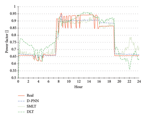
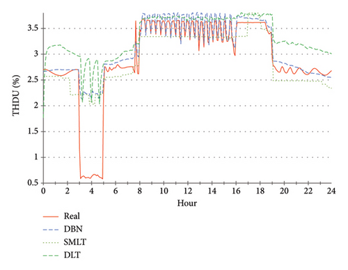
The described DBN, DLT and SMLT modelling techniques used the presented training scheme (Figure 3) to predict the operative characteristics in daily PQ. The models process the same types of forecast series for unknown binary load of attached 4-consumers which determine the user demands at the switching times, including the decimal code and sample time (13 data input in total). The learnt PQ output is computed 24 h ahead in one-sequenced processing, which reduces the time consumption. Figures 9, 10, 11, 12, 13 demonstrate the prediction of PQ compared to data measurements on selected specific days in the examination time of summer. The described verification of PQ evaluates user-adaptable algorithmically composed power consumption scenarios on a RE day basis optimisation.

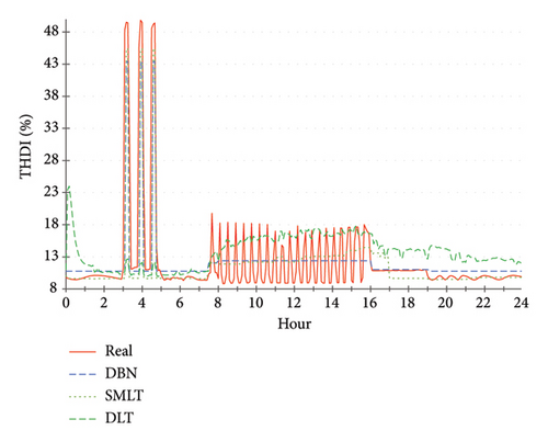
Long-time NWP archives are generally not available (not recorded as observational data), so the complete forecast set is missing in the monthly repository set⁵. Observational data were noised for this reason to simulate 24 h forecast series. The related real-world observations of the meta-input were randomly disturbed in the 20% tolerance range to apply only adequate changes in the defined base limit of the values. The 5% extra limit on next-time sequence variations (+ or −) in the real data guarantees not to exceed the 5% alterations range and produces a continuous smooth-noised output (resembling forecasted data). The SMLT random function can be used alternatively to generate response variables perturbed by random noise with distribution statistics for a linearly generalised model².

8. PQ Day Validation Processing NWP: Evaluation of Experiments and Interpretation of Results

Figures 14, 15, 16 summarise the daily avg. predictive RMSEs for U, PF, and P in the experimental period. An evident increase in modelling inaccuracies of all the applied techniques in U in the first few days (Figure 14) is probably a result of variability in an uncertain environment (few available training days) or U data specifics. Their weak representation in the half-beginning period of the archive set⁵ used in training does not comprise direct relationships with meteorological patterns, essential for processing unseen 24 h forecast data (Table 1). The parameter freq. has stable time behaviour, including only insignificant flows within the acceptable interval limits⁵.

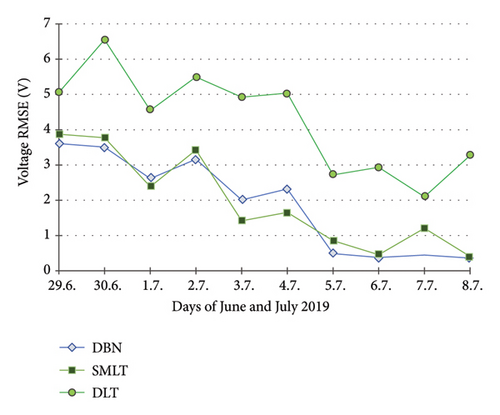
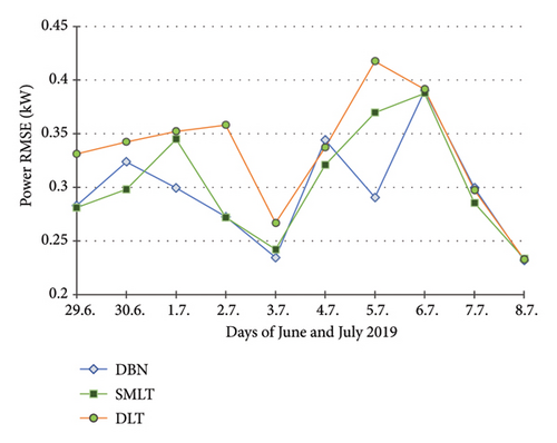
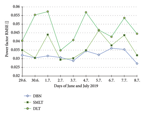
The THDU series show a high correlation with PF, so the predictive modelling was not completed for this parameter (Figure 12). The THDU day approximate cycles look like those of the PF at error output (Figure 16). A day demo estimate of THDI is shown in Figure 13. It was not performed throughout the experimental PQ period for this less significant parameter. U is a critical metric in PQ evaluations, influencing both the operational efficiency of electrical systems and the reliability of the power supply. The DLT U prediction falls in the averaging of historical data, leading to a loss of critical pattern information (Figure 14). Significant inaccuracies are especially found at the beginning of the prediction timeline. This approach may not be suitable for predicting parameters that exhibit high variability or nonlinear characteristics, such as U. It suggests that the fundamental DLT structure is conducive to capturing the complexities of U dynamics. Previous studies indicated that DLT can struggle with temporal dependencies and abrupt changes in data patterns, which are common in power systems [31]. Despite attempts to adjust training and testing parameters or network architecture, no improvements in predictive accuracy have been achieved. Unlike DLT, other probabilistic and ensemble learning techniques have shown superior performance in predicting the U voltage. The predictive results of all models show a high correlation in U, PF and P (Figures 14, 15, 16). Small variations in the accuracy of the SMLT are additionally related to DLT in the less precise estimate of PF in the middle term times (Figure 16). DLT modelling in P yields a similar approximation, compared to the predictive accuracy of other applied techniques (Figure 15). Daily errors tend to a slight decrease in all PQ parameters, continuously in U. These improvements are naturally the result of an increasing number of training samples available on each next prediction day. This implies better results by using applicable records in larger archive databases. Table 3 summarises the predictive accuracy of the compared modelling techniques.

EBaggT aggregates were recognised as the most successful SMLT models in 24 h prediction of series of U, PF parameters (Figures 9 and 11). EBoosT was recognised as more efficient in daily estimation of the P parameter in most experiments compared to the analogous EBaggT (Figure 15)². Binary element trees are hierarchical structures in which each internal node represents a decision based on a predictor variable and each leaf node corresponds to a predicted outcome. Bagging creates multiple subsets of the training data by sampling with replacement and fitting each regression tree of the ensemble to a subset. Boosting focusses on sequentially fitting trees, where each new one is trained to correct the errors made by the previous solvers. This method assigns higher weights to misclassified observations, allowing the ensemble to focus on problem cases³. GPR is a nonparametric Bayesian regression, that is, effective especially in modelling uncertainties in nonlinear relationships. The choice of kernel function is crucial, as it defines a covariance structure of the underlying data⁴. The predictive performance of the GPR models in PF was consistent with the best modelling accuracy in the day experiments, strengthening the robustness of the Matern kernel in its applications (Table 4).

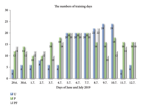
DLT normalises predictor values in training and testing data for unit and mean zero variances. The nominal deviation in the data characteristics is calculated for the input samples¹. The DBN models are verified step by step for each modification or extension. Evolutionary DfL modelling allows adequate changes in BT structure, node and transform module selection, parameter updates in continuous testing, usually leading to optimal problem solutions. Figure 17 presents initialisation times of the models in detection of the minimal errors. Optimal data samples help to obtain higher predictive accuracy under complicated conditions or dynamical PQ progress, improving day-to-day operational planning.

The PQ parameters alternate in characteristic daytime amplitudes, primarily determined by a specific 4-combination load time shift. Changes in shape harmonics are related to various factors, mostly PVP production capacity and system stability in specific recharging modes (Figures 9, 10, 11, 12, 13). Ramp-step variations in PQ cycles are mostly the result of switching user demand events in combined active load events. The rapid spike uncertainty in tP, PF, THDU, and THDI leads to only partial approximation ability of the applied computing techniques. Their models only average data for the learnt PQ progress in highly intermitted nature events. The observed increase in errors in the results of the U, P, and slightly PF models in the first examination stage can be attributed to two primary factors: The uncertainty associated with the prevailing weather instabilities and consequent inadequacy of the data patterns used in training, leading to partial applicability of the model. And the second one: A weak representation of the PQ characteristics⁵ results in inefficiency in learning from the observational data in the first prediction period. The PF and THDU parameters of PQ are specifically correlated within the cycle day progress (Figures 11 and 12). The Freq is a major parameter in PQ with stable behaviour over the monitored time characterised by insignificant tiny variations. These instabilities are presumably induced by measurement or recording instruments or system anomalies. The variations observed in the PQ series are not Freq-correlated, like the operating load modes. These minor discrepancies are considered negligible deviations and do not warrant in-depth analysis in predictive modelling.

9. Discussion

NWP series in the last processing stage compensates for the eventual discrepancies between training and predictive patterns in occasional over-changes. NWP utilities (based on a physical consideration) mostly overcome the self-standing performance of modelling statistics in a mid-term horizon. Self-adaptation computing is based on the search of historical data for relevant patterns that may miss potentially emerging disturbing, or abnormal fault cases. Significant data samples may not be included in the available repository set, causing shortcomings and flaws in statistical learning. AI-based strategies can benefit from processing big data and their ability to learn from predictive errors or reinterpret potential misfires. Fully self-optimising DfL was applied without any adaptation to the problem specifics, it can model a variety of undefined systems described by data. Its node-by-node input couple selection in the production of PDE components allows efficient feature extraction without loss in data dimensionality. The DBN structure is progressively expanded to dynamically reflect pattern progress and complexity (as compared to traditional fixed architectures). Its PDE components gain is re-evaluated in each training cycle in refining the model, though several-level reoptimalisation increases naturally computing and algorithmic costs. The DfL modular concept allows for incremental training that is keeping previously learnt knowledge of the models in learning new data relations available in the forthcoming computing days. The model initialisation time can be detected on extensive databases, relating the prediction horizon, as different patterns are usable/adequate in short- or long-term intervals. The regional routine NWP is usually freely available but is a few hours delayed due to higher computing costs in numerical simulations. Inadequate adaptation of NWP output to adjacent layers in local turbulence to cause AI statistics magnifies local forecasting errors or parametric inaccuracies [4]. NWP postprocessing is sparsely less precise because of spatial interpolation on mesoscales. The optimal NWP model could be chosen from several different implementations of physical atmospheric processes according to the efficiency evaluated in several subsequent days, avoiding prediction. This selection can compensate for local phenomena and reduce uncertainties in simulations. Elaborated combinatorial coding in binary active equipment can contribute to a better definition of load modes. A better identification of the operational status could strengthen the robustness of the prediction models. NWP data are supplied by a system independent of computing statistics, and the added value in problem-diverse representation contributes to better stability in AI modelling. Efficient training is mainly dependent on the consistency of day-sampling and prediction intervals. The predictability of new patterns in processing new NWP replacements is further influenced by various types of (potentially ambiguous) evaluated load combinatorial schemes. Signal-first processing was not applied to PQ data whose denoising or transform analysis can improve the results.

10. Conclusions

As a key finding, the proposed NWP-based hybrid approach examined on a small month data set allows for early PQ verification up to 48 h at a daily time, guaranteed in unexpected surroundings and charge states. Optimal scheduling of user-adaptive demands determines operational grid stability. Predictive postprocessing integrates statistical learning with NWP, reducing unexpected model flaws in turnover disturbances. The DBN models proved their efficiency in capturing high variability and ambiguity in patterns, producing regular PQ output. The DfL self-evolution is distinguished by a high combinatorial diversity of modular composite PDE solutions that reflect unexpected dynamical load and condition states in processing unseen NWP output. The best applicable SMLT models were the ensemble trees and GPR. Their probabilistic and aggregative framework compensates for a higher uncertainty in calculating off-grid PQ, caused by the intermittent nature of RE and consequent system anomalies. Efficient SMLT methods (EBaggT/EBoosT, GPR) usually produce a comparable test and prediction output. Several applicable scenarios of engaged appliances can be offered and chosen on demand, according to adaptable PQ optimising plans. In future research, automatic load scheduling can be implemented to algorithmically synchronise active power consumers in the effective next-day operation with respect to RE availability and recharging. This strategy reveals possible collisions in load modes that can result in system instabilities. The proposed 2-level PQ optimisation requires first reliable estimates of RE daily production capacity in secondary processing NWP output to control daily load. 100% continuous backup storage is largely inaccessible; however, its continuous tracking in recharging with respect to excessive RE is to be covered in future studies. An integrated online 1–48 h intelligent PQ prediction system (based on NWP support) is planned to be implemented in the smart testing facility (Figure 2). The input-output time delay can be set according to the availability of NWP series to refine the first all-day plans. No additional adaptation is needed to accommodate different time horizons. The test allocated data is increased proportionally to the predictive time to account for computational uncertainty.

Ethics Statement

This study was compliance with Ethical Standards.

Conflicts of Interest

The author declares no conflicts of interest.

Funding

This work was supported by Vysoká Škola Bánská - Technická Univerzita Ostrava, SP2025/016.

Endnotes

¹MATLAB—Deep Learning tool-box for sequence to sequence regression (DLT): https://www.mathworks.com/help/deeplearning/ug/sequence-to-sequence-regression-using-deep-learning.html

²MATLAB—Statistics and Machine Learning tool-box for regression (SMLT) https://www.mathworks.com/help/stats/choose-regression-model-options.html, https://mathworks.com/help/stats/select-data-and-validation-for-regression-problem.html

³MATLAB—Ensemble algorithms https://www.mathworks.com/help/stats/ensemble-algorithms.html

⁴MATLAB—Gaussian Process Regression (GPR) models https://www.mathworks.com/help/stats/gaussian-process-regression-models.html, https://www.mathworks.com/help/stats/kernel-covariance-function-options.html

⁵DBN application C++ parametric software, Weather & PQ data: https://drive.google.com/drive/folders/1ZAw8KcvDEDM-i7ifVe_hDoS35nI64-Fh?usp=sharing, https://nextcloud.vsb.cz/s/EFDJ7mRyxfHkjSc